Emergent irreversibility and entanglement spectrum statistics

Abstract

We study the problem of irreversibility when the dynamical evolution of a many-body system is described by a stochastic quantum circuit. Such evolution is more general than a Hamiltonian one, and since energy levels are not well defined, the well-established connection between the statistical fluctuations of the energy spectrum and irreversibility cannot be made. We show that the entanglement spectrum provides a more general connection. Irreversibility is marked by a failure of a disentangling algorithm and is preceded by the appearance of Wigner-Dyson statistical fluctuations in the entanglement spectrum. This analysis can be done at the wave-function level and offers an alternative route to study quantum chaos and quantum integrability.

In closed quantum systems, evolution is unitary and both irreversibility and nonintegrability are elusive notions. Because of unitarity, evolution is always stable under errors in initial conditions. Thus, in quantum mechanics irreversibility is defined by the vanishing of the probability (known as fidelity) of returning to an initial state under arbitrarily small imperfections in the Hamiltonian during the reversed time evolution Peres84 . Nonintegrability is associated to a Wigner-Dyson distribution of the energy-level spacings that shows level repulsion gutzwiller and nonintegrable Hamiltonians in this context are irreversible. Integrable Hamiltonians, instead, tend to show clustering of energy levels but can be either reversible or irreversible znidaric ; benenti . When the time evolution is not governed by a Hamiltonian, or when the Hamiltonian is time dependent, energy levels are not well defined and these associations cease to be meaningful. How can one relate nonintegrability and irreversibility in these more general cases of quantum evolution?

In this Letter we show that one can answer this question by looking at the wave function alone. This route allows one to study generic quantum evolutions even when energy is not well defined. We show that by studying the level statistics of the entanglement spectrum one can determine whether the evolution is irreversible or not through a protocol that we call entanglement cooling. It turns out that the onset of irreversibility is marked by the presence of Wigner-Dyson statistics in the entanglement spectrum.

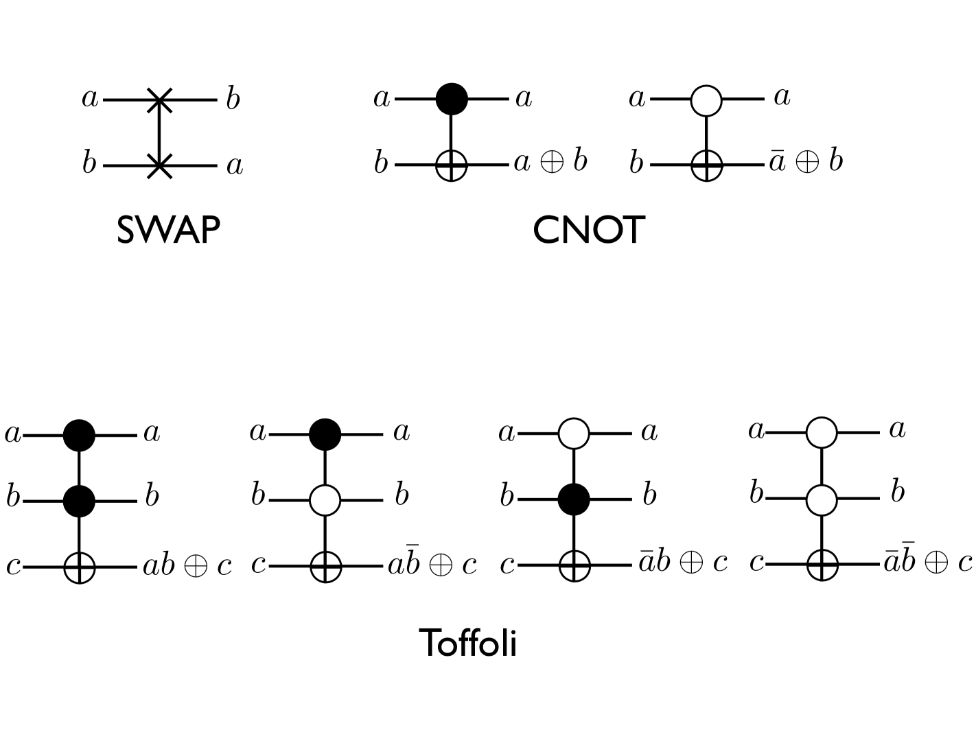
Figure 1: Reversible gates used in the quantum stochastic evolutions. The output values of the gates are defined when $a$, $b$, and $c$ take values 0 and 1. Top row: Two-qubit gates SWAP and CNOT. Bottom row: The different variations of the three-qubit Toffoli gates. We note that different variations of the CNOT and Toffoli gates can be obtained from one fixed variation plus NOT gates.

The quantum system we consider contains $n$ qubits and evolves unitarily from an initial factorized state of the form $|\Psi_{0}\rangle=|\psi_{1}\rangle\otimes|\psi_{2}\rangle\otimes\cdots\otimes|\psi_{n}\rangle$ where each single-qubit state is defined as $|\psi_{j}\rangle=\cos({\theta_{j}}/{2})|0\rangle+\sin({\theta_{j}}/{2})e^{i\phi_{j}}|1\rangle$, with $\theta_{j}$ and $\phi_{j}$ arbitrary. Formally, the evolution is obtained by applying a unitary matrix $U$ to the state vector, $|\Psi_{t}\rangle=U|\Psi_{0}\rangle=\sum_{x}\Psi_{t}(x)\,|x\rangle$, where the states $|x\rangle\equiv|x_{1}\,x_{2}\dots x_{n}\rangle$ form the computational basis, with $x_{j}=0,1$ for $j=1,\dots,n$. Using the language of quantum computing, we assume that this unitary matrix is represented by gates. We recall that the two-qubit CNOT gate and arbitrary one-qubit rotations are sufficient for universal quantum computing divincenzo95 . In what follows, we shall restrict the gates to the permutation group, which is a subgroup of the unitary group. The restriction to the permutation subgroup of unitary transformations allows for a much more efficient computation of the state of the system as it evolves with gates. In particular, we consider the unitary gates in the set $\mathcal{I}_{3}=\{\mbox{SWAP},\mbox{CNOT},\mbox{Toffoli}\}$ depicted in Fig. 1. We build a stochastic quantum circuit $U=\prod_{k}^{M}U_{k}$ by drawing randomly with uniform probability pairs or triplets of qubits and a random gate $U_{k}\in\mathcal{I}_{3}$ with probability $1/3$. We remark that the Toffoli gate alone is sufficient for universal classical computation toffoli . We also consider more restricted (and nonuniversal) circuits obtained by employing only gates in the set $\mathcal{I}_{2}=\{\mbox{SWAP},\mbox{CNOT}\}$.

At each step $k$ of the circuit, the $n$ qubits are partitioned into subsystems $(A,B)$ with $n_{A}$ and $n_{B}$ qubits, and the entanglement properties of the system are obtained through the singular values $\lambda_{k}>0$, $k=1\ldots,r$, which result from the Schmidt decomposition ekert ; peres of the state $|\Psi_{t}\rangle=\sum_{k=1}^{r}\lambda_{k}\;|\psi^{A}_{t\,(k)}\rangle\otimes|\psi^{B}_{t\,(k)}\rangle$. The reduced density matrices $\rho_{A}=\mbox{tr}_{B}(|\Psi_{t}\rangle\langle\Psi_{t}|)$ and $\rho_{B}=\mbox{tr}_{A}(|\Psi_{t}\rangle\langle\Psi_{t}|)$ have eigenvalues $\{p_{k}=\lambda_{k}^{2}\}$. These $p_{k}$ define a probability distribution whose Rényi entropies are defined as renyi61

$$S_{q}(n_{A},n_{B})=\frac{1}{1-q}\,\log_{2}\sum_{k=1}^{r}p_{k}^{q}\,,$$ (1)

with $\sum_{k=1}^{r}p_{k}=1$. The zeroth Rényi entropy is related to the rank, namely, the number $r$ of nonzero singular values, $S_{0}=\log_{2}r$. The $q=1$ Rényi entropy is the Shannon entropy measuring the amount of information in the distribution $\{p_{k}\}$: $S_{1}=-\sum_{k}p_{k}\log_{2}p_{k}$.

What happens to entanglement during the evolution with gates? One can show that, under a generic stochastic random circuit, entanglement grows linearly with time, and then saturates to its maximum possible value asz ; chamon2012 . This occurs typically, meaning that the probability of having a different outcome is zero in the thermodynamic limit. A similar behavior is obtained also for the restricted quantum evolutions considered here, whether one uses two- or three-qubit gates. The saturation value is typically reached after about $M\sim n^{2}$ transformations. In Fig. 2, we see a numerical simulation of the protocol used, with both two-qubit and three-qubit gates, which confirms this scenario. We call this part of the protocol “entanglement heating.”

Because entanglement increases with the number of gates, in order to revert the evolution to return back to the initial state, it is natural to attempt an algorithm that completely disentangles the system. The entanglement entropies provide a natural metric to use in a minimization process. If one is able to remove all the entanglement while recording the moves that led to the decreases, one builds one possible reverse algorithm that takes the system from the final state back to the initial (product) state. In practice, we implement such disentangling or “entropy cooling” algorithm as follows. We attempt a gate, chosen at random, and compute the change in entanglement entropy. Then we decide whether or not to accept this gate into the sequence according to a Metropolis algorithm: if the entanglement goes down, we always take this move; if not, we take it with a certain probability, which we decrease as function of the number of attempts (similarly to simulated annealing, but applied to entanglement entropy and not energy). More precisely, we use as the optimization function the sum of the entanglement entropies over all bipartitions of the system into $n_{A}$ and $n_{B}$ consecutive qubits with $n_{A}+n_{B}=n$, namely, ${\cal S}_{q}=\sum_{n_{A}=1}^{n-1}S_{q}(n_{A},n_{B})$. The reason for this choice is that a single bipartition is sensitive only to gates that act on qubits in both subsystems $A$ and $B$. However, if one considers the sums over the entanglement for all bipartitions, one is sensitive to all reductions in entanglement, no matter where the gates act.

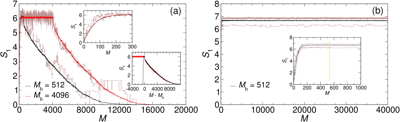
Figure 2: (Color online) Evolution of the entanglement entropy $S_{1}$ obtained from the bipartition of the qubit string at the middle ($n_{A}=n_{B}=8$) as function of the number of applied gates. First, $M_{\rm h}$ reversible gates are randomly applied (heating period); second, a Metropolis algorithm is used to reverse the evolution and restore zero entropy (cooldown period). The solid black ($M_{\rm h}=512$) and red ($M_{\rm h}=4096$) lines result from averaging $S_{1}$ over 128 initial-state realizations. The brown lines show the evolution of $S_{1}$ for two typical realizations. (a) Only two-qubit gates are used. Upper inset: The heating period. Lower inset: Shifted curves, showing that the cooling, on average, is independent of the duration of the heating period. (b) A mixture of two-qubit and Toffoli gates is used. Inset: Detail of the transition between heating and cooling periods. The dashed line indicates the transition point.

The resulting $q=1$ Rényi entropy as a function of the gate number for a given sequence of the algorithm using only the gates in $\mathcal{I}_{2}$ is shown in Fig. 2(a). The data show two examples of the entanglement evolution for two particular “heating” and “cooling” runs, as well as the average of 128 different realizations with random initial product states for 16 qubits, with each $\theta_{j}$ randomly picked from the interval $[0,\pi]$, and $\phi_{j}=0,\pi$ (thus focusing on real wave functions). We show data for the case when the system is entangled with 512 and with 4096 gates. The system is “cooled” by minimizing ${\cal S}_{0}$ (similar results are obtained when minimizing ${\cal S}_{2}$). Notice that the “cooling” time for the average curve does not depend on how long the system was “heated,” provided that the same maximum entanglement entropy is reached. The disentangling algorithm works for all individual realizations of the protocol. We were always able to reverse to a completely factorized tensor product state with zero entanglement. This is quite remarkable, because the success of the algorithm does not depend at all on the amount of the entanglement produced. So one may wonder whether every quantum circuit can be reversed with such a cooling protocol.

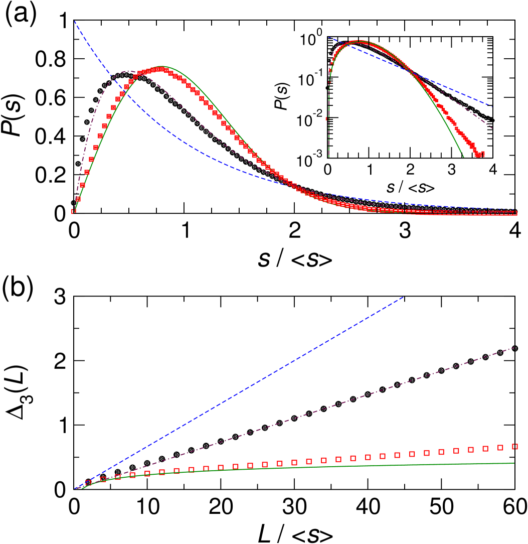
Figure 3: (Color online) (a) The distribution of the spacing between consecutive unfolded singular values obtained from a bipartition at the middle of a $n=16$ qubit string at the end of the heating period ($M_{\rm h}=512$). Solid black circles are for two-qubit gate heating and open red squares are for heating with a mixture of two-qubit and Toffoli gates. Solid green line: GOE prediction. Dashed blue line: Poisson distribution. Dotted-dashed maroon line: Semi-Poisson distribution. Inset: The tail of the distributions. (b) The average spectral rigidity $\Delta_{3}(L)$ obtained from the same spectra (a linear fit is used for the semi-Poisson line). A total of 5000 realizations were used to compute the averages.

To answer this question, consider now the case when entanglement entropy “heating” involves the gates in $\mathcal{I}_{3}$. Then, apply the disentangling algorithm using the same set of gates. For all realizations studied, we find that it is never possible to completely disentangle the state using the Metropolis protocol described above note1 . In Fig. 2(b) we show two typical realizations of the heating and cooling protocol, with a random initial product state and 512 random gate sequences for the heating phase. We also show the average over 128 realizations.

And yet, by only looking at the amount of entanglement generated upon “heating,” we cannot tell whether the evolution is reversible by the cooling algorithm. As we have shown, by heating with either two-qubit gates or a mixture of two-qubit and Toffoli gates, one rapidly reaches an almost maximally entangled state. Nevertheless, only for the former are we able to reverse the system back into a product-state form. Indeed, it is known that most states in the Hilbert space are maximally entangled, and that generic quantum evolutions will eventually lead to an almost maximally entangled state page ; emerson ; viola ; asz . This happens even under quantum quench with an integrable Hamiltonian calabrese .

What is in the entanglement, which is not the entanglement entropy, that tells us whether a quantum evolution is reversible or not? The answer lies in the statistics of the levels $\{p_{k}\}$ in the entanglement spectrum. We have computed the entanglement spectrum of the qubit string at the end of the heating period. The spectrum is obtained from the singular values resulting from the Schmidt decomposition of the quantum state upon bipartitioning of the qubit string in the middle (i.e., $n_{A}=n_{B}=n/2)$. The spectrum is first unfolded to yield a constant density before the statistical analysis is performed (see the Appendix for a detailed description of the unfolding procedure). In Fig. 3(a) we show the distribution of the spacings between adjacent singular values for reversible cases (heating period performed with $\mathcal{I}_{2}$ gates) and irreversible ones (heating period performed with $\mathcal{I}_{3}$ gates). The difference is striking: while the data points for the irreversible case match quite closely the distribution of spacings of the Gaussian orthogonal ensemble (GOE) of random matrices mehtabook , the data points for the reversible case show a weaker repulsion and follow the so-called semi-Poisson statistics, which has been proposed for the energy spectra of systems at metal-insulator transitions bogomolny . The difference in behavior is also manifest in the spectral rigidity function $\Delta_{3}(L)$, which measures, for a given interval $L$, the least-square deviation of the spectral staircase from the best-fitting straight line dyson1963 . In Fig. 3b, long-range correlations are much stronger in the irreversible case, with the data points also falling close to the GOE prediction. For the reversible case, the singular values are much less correlated and the spectrum much less rigid. This indicates that the statistical fluctuations of the entanglement spectra of irreversible systems are similar to those observed in the energy spectrum of the so-called quantum chaotic systems gutzwiller .

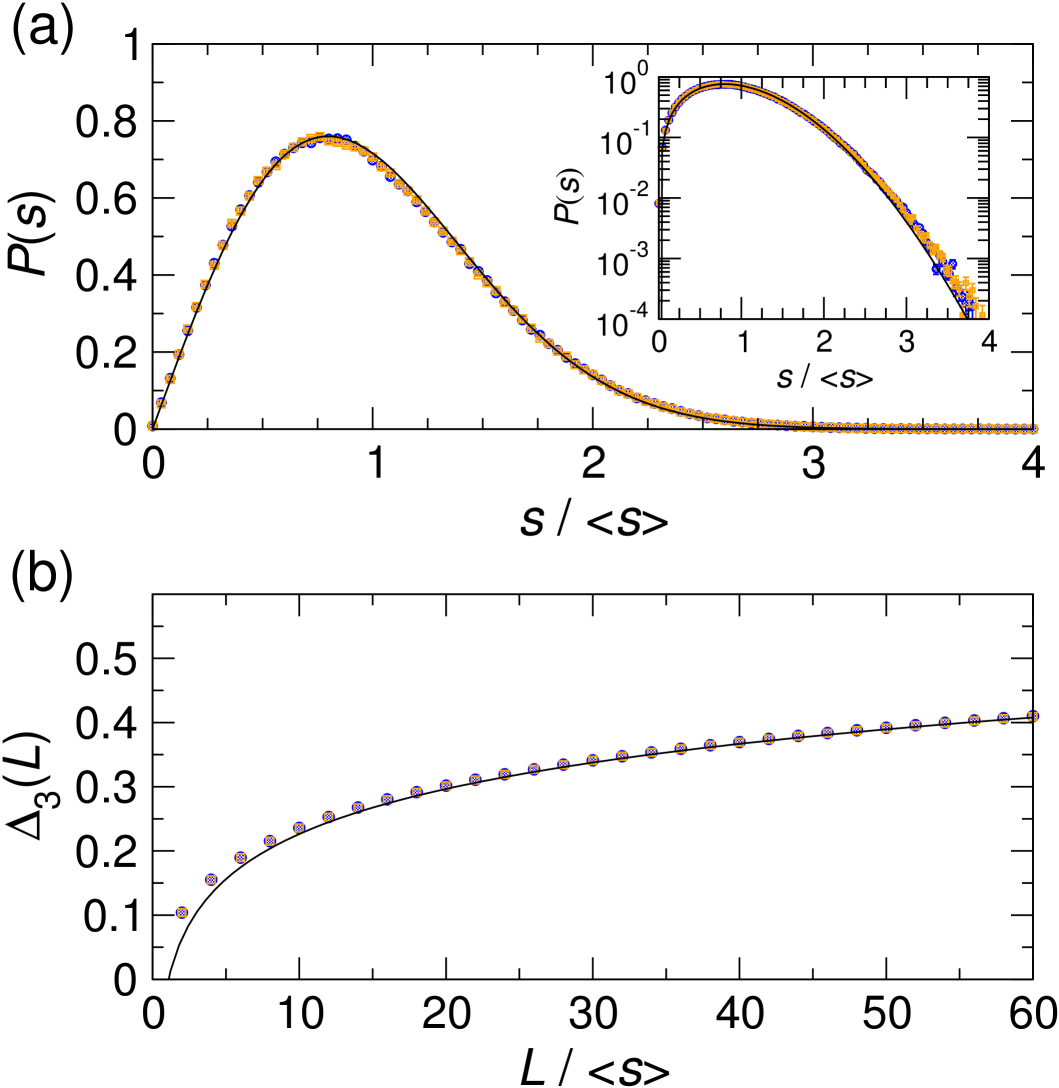
Figure 4: (Color online) The statistical fluctuations of the entanglement spectrum for initial product states $|\chi^{(1)}\rangle$ (orange empty squares) and $|\chi^{(2)}\rangle$ (blue full circles) entangled with a mixture of two-qubit and Toffoli gates ($n=16$, $M_{\rm h}=512$). The solid green line is the GOE prediction. (a) Distribution of unfolded singular value spacings. Inset: distribution tails. (b) Average spectral rigidity $\Delta_{3}(L)$. Statistical averages performed over 5000 realizations.

In Fig. 4 we also show the entanglement level statistics for the particular case when one starts with initial factorized states of the form $|\chi^{(k)}\rangle=|\psi_{1}^{(k)}\rangle\otimes|\psi_{2}^{(k)}\rangle\otimes\cdots\otimes|\psi_{n}^{(k)}\rangle$, $k=1,2$, where $|\psi_{1}^{(1)}\rangle=|0\rangle$ and $|\psi_{j}^{(1)}\rangle=(|0\rangle+|1\rangle)/\sqrt{2}$ for $j=2,\ldots,n$, and $|\psi_{j}^{(2)}\rangle=(|0\rangle-|1\rangle)/\sqrt{2}$ for $j=1,\ldots,n$. We evolve these $n=16$-bit states with $M=512$ gates chosen randomly from the set $\mathcal{I}_{3}$. The data in Fig. 4 clearly conform to the GOE statistics, and we observe that the disentangling algorithm again fails, indicating that reversing the computation is extremely difficult.

In quantum mechanics, irreversibility, chaos, nonintegrability and thermalization are phenomena often associated with one another. Unfortunately, some of these notions are ill defined, such as integrability and lack thereof, and the associations are either weak or plagued by counterexamples. For instance, irreversibility can be associated to both chaotic and nonchaotic Hamiltonians znidaric ; benenti and there are nonintegrable systems that do not thermalize eisert . Moreover, some of these concepts are only defined in the context of time-independent Hamiltonian evolutions. For instance, the energy levels of a chaotic Hamiltonian show Wigner-Dyson statistics.

In this Letter we presented an alternative approach to the question of irreversibility and complex behavior in quantum systems that works purely at the wave-function level. We did so by studying the eigenvalues of the reduced density matrix of a subsystem, the so-called entanglement spectrum footnote . We showed that (i) a disentangling Metropolis algorithm provides a firm notion of reversibility, namely, the evolution can be inverted if the state can be disentangled, and (ii) irreversibility arises when the level statistics of the entanglement spectrum of a subsystem is Wigner-Dyson.

On the other hand, in the example we studied where the spectrum did not follow Wigner-Dyson statistics, we were always capable of reverting the evolution, even with zero knowledge about the quantum circuit. It is remarkable that the length of the reverted circuit does not depend on the length of the initial circuit, as long as the maximum entanglement entropy is reached. In the disentangling algorithm, we obtained similar results with the Rényi entropy $S_{2}$. This is remarkable because $S_{2}$ is an observable that can be measured s1 ; s2b , for example, in optical lattices with ultracold atomic gases bloch .

The results of this work motivate several questions and applications. The method presented here is applicable to any kind of quantum evolution, regardless of whether it comes from a quantum circuit, a time-dependent or -independent Hamiltonian system, or an open quantum system. First of all, we can examine the behavior of the entanglement level spacing statistics in integrable Hamiltonian models both in the ground state or during the time evolution after a quantum quench. Using techniques such as the density matrix renormalization group, one can study these models once integrability is broken. We believe that our approach can shed new light on the notion of integrability and lack thereof in quantum systems. The possibility of studying quantum systems away from equilibrium and their universal properties in dynamical phase transitions polkovnikov and many-body localization boris ; huse ; refael is another feature of the method that only involves wave functions. Similarly, we can study the behavior of the entanglement level spacing statistics at critical points of integrable and nonintegrable systems entmanybody ; arul . The adiabaticity of time-dependent quantum processes zurek can be examined under the lens of the entanglement spectrum as well, with potential applications to adiabatic quantum computing. Moreover, one can study how the complexity of the entanglement spectrum is related to quantum algorithms capable of giving an exponential speedup arul2 . Under the same lens of the entanglement spectrum, one should study the typicality of quantum chaos in random states vinayak ; zic . Entanglement is very ubiquitous in the Hilbert space zic ; emerson , and while this feature has been crucial to show the typicality of thermalization in closed quantum systems nature , this also means that entanglement entropy is unable to characterize quantum irreversibility, and the difference between integrable and nonintegrable systems. Our results show that the understanding of complex quantum behavior lies in the statistics of the fluctuations of the entanglement level spacing.

We acknowledge financial support from the U.S. National Science Foundation through grants CCF 1116590 and CCF 1117241, and by the National Basic Research Program of China Grant 2011CBA00300, 2011CBA00301, the National Natural Science Foundation of China Grant 61033001, 61361136003.

Appendix: Spectral analysis

Before computing the statistical properties of the singular values ${\lambda_{k}}$, ${k=1,\ldots,d}$, the spectrum must be unfolded in such a way to produce a new sequence ${s_{k}=f(\lambda_{k})}$, ${k=1,\ldots,d}$, with a uniform density. In Fig. 1 we show typical spectra obtained for $n=16$ qubit systems after a heating period of 512 gates and starting from a random initial state. For the cases where the initial state has amplitudes $W(x)$ taking continuous values (in the set of real numbers), both small and large jumps appear in some spectra, particularly for the case of circuits involving only two-bit permutation gates. We thus divided the spectrum of each realization into segments and fitted to each segment an independent polynomial function (see Fig. 1). Segments shorter than 10 singular values were not considered and singular values near the beginning or the end of the spectrum were discarded. For the cases of initial states with discrete amplitudes, namely, $W(x)=0,1$ or $W(x)=\pm 1$, the spectra are quite smooth (see Fig. 2) and follow accurately a Marchenko-Pastur distribution, which can be derived from the semi-circle eigenvalue distribution of Random Matrix Theory:

$$s_{k} = \frac{4}{\pi}\int_{x_{k}}^{1}dx\,\sqrt{1-x^{2}}$$ (2)

$$= 1-\frac{2}{\pi}\left[x_{k}\sqrt{1-x_{k}^{2}}+{\rm arcsin}(x_{k})\right],$$ (3)

where $x_{k}^{2}=\lambda_{k}^{2}\,d/4Z(1-p_{1})$ and $Z=\sum_{k=1}^{d}\lambda_{k}^{2}$. Here, $p_{1}$ is the probability of choosing an initial amplitude $W=1$. In these cases, the unfolding was done with the same continuous curve for all realizations.

The distribution of spacings, $P(s)$, where $s=s_{k+1}-s_{k}$, accounts for short-range correlation and repulsion. Results were compared to the Poisson and GOE predictions (we did not need to consider other ensembles because only the entanglement entropy of states with real amplitudes were analyzed): $P_{\rm Poisson}(s)=(1/\Delta)\exp(-s/\Delta)$ and $P_{\rm GOE}(s)=\frac{\pi}{2}\,(s/\Delta^{2})\,\exp(-\pi s^{2}/4\Delta^{2})$, where $\Delta=\langle s\rangle$.

The spectral rigidity was quantified through the function

$$\Delta_{3}(L)=\frac{1}{L}\left\langle{\rm min}_{a,b}\int_{-L/2}^{L/2}dS\,\left[N(S+S_{0})-(a+bS)\right]^{2}\right\rangle_{S_{0}},$$ (4)

where

$$N(S)=\sum_{k=1}^{d}\theta(S-s_{k})$$ (5)

is the spectral staircase. Notice that for a given value of the interval $L$, the averaging also involves sweeping over the spectrum by varying the center point $S_{0}$. The results were compared with the Poisson and GOE predictions, namely, $\Delta_{3}^{\rm Poisson}(L)=L/(15\Delta)$ and $\Delta_{3}^{\rm GOE}(L)=\ln(L/\Delta)/\pi^{2}-0.00696$ for $L\gg\Delta$.

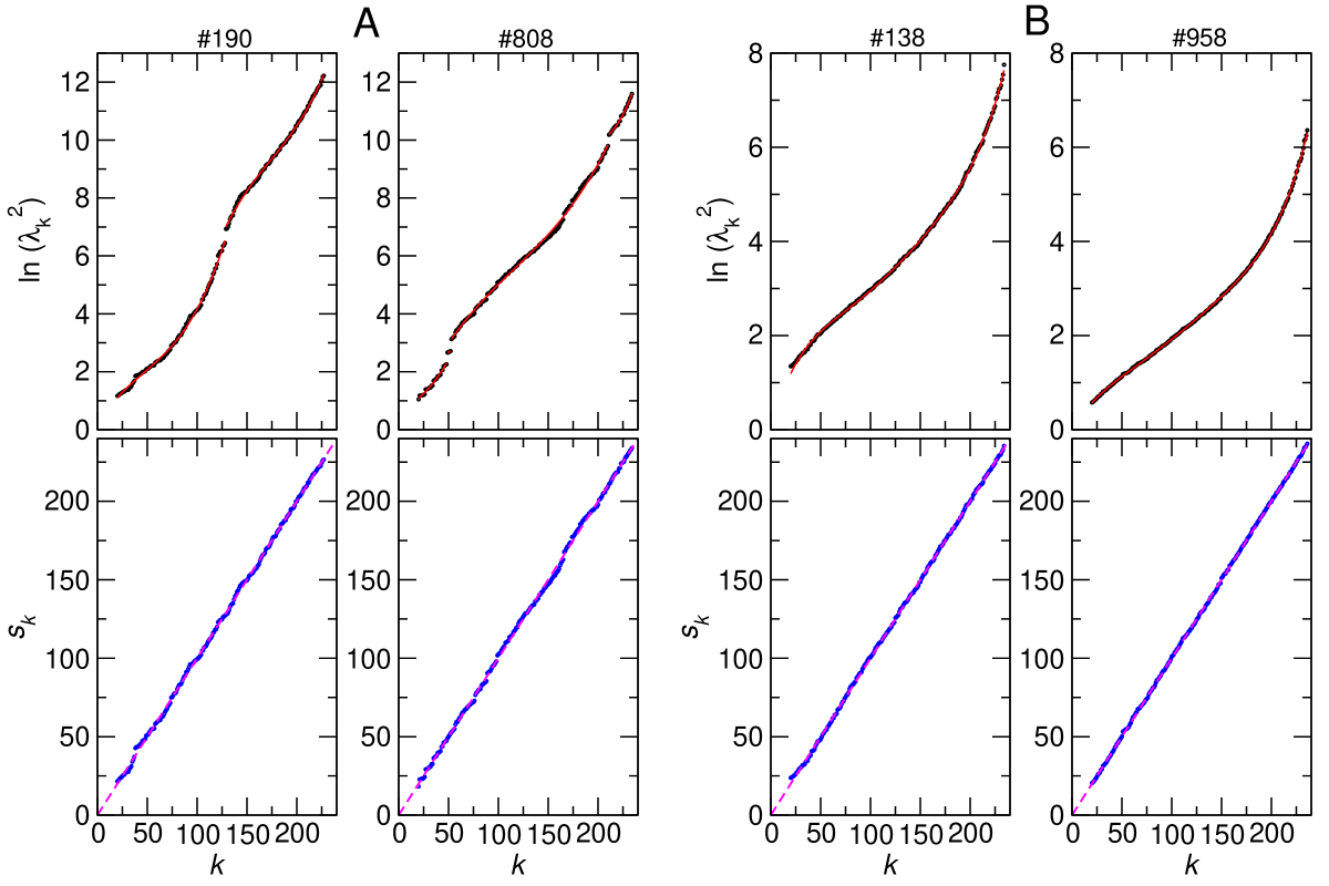
Figure 5: (a) Upper panels: examples of the entanglement spectra obtained by evolving a $n=16$ qubit system with 512 random two-bit reversible gates starting from two different initial states with a continuous distribution of amplitudes (sample numbers are indicated at the top of the graphs). Black circles represent the raw data and the solid red line is the result of a multi-segment polynomial fit (third degree). Lower panels: the blue circles are the resulting unfolded spectrum. The magenta dashed line is a guide to the eye, showing how close the distribution is to a straight line. (b) Similar to (a), but for states evolved with a mixture of reversible two- and three-bit (Toffoli) gates.

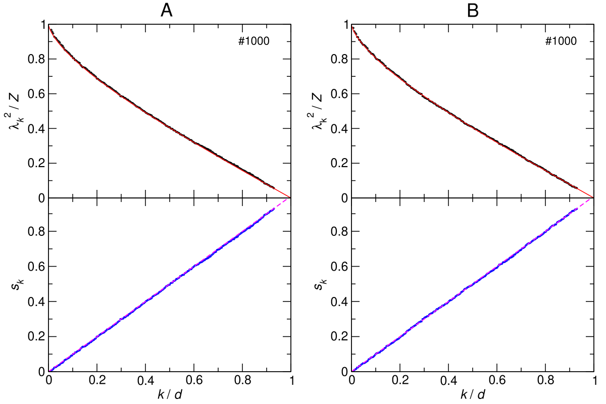
Figure 6: (a) Upper panels: example of the entanglement spectra obtained by evolving a $n=16$ ($d=256$) qubit system with a mixture of 512 random reversible two- and three-bit (Toffoli) gates starting from an initial states with a discrete distribution of amplitudes, namely, $W(x)=0,1$. Black circles represent the raw data and the solid red line indicates $k/d=1-(2/\pi)[x_{k}\sqrt{(}1-x_{k}^{2})-{\rm asin}(x_{k})]$, with $x_{k}=\lambda_{k}^{2}/Z$ and $Z=\sum_{k=1}^{d}\lambda_{k}^{2}$. Lower panels: the blue circles are the resulting unfolded spectrum. The magenta dashed is a guide to the eye, showing how close the distribution is to a straight line. (b) Similar to (a), but for initial states with a distribution of amplitudes $W(x)=\pm 1$.

References

- (1) J.-S. Caux and J. Mossel, J. Stat. Mech. (2011) P02023.
- (2) A. Peres, Phys. Rev. A 30, 1610 (1984).
- (3) M. C. Gutzwiller, Chaos in Classical and Quantum Mechanics (Springer Verlag, New York, 1991).
- (4) T. Gorin, T. Prosen, T.H. Seligman, and M. Žnidarič, Phys. Rep. 435, 33 (2006).
- (5) G. Benenti and G. Casati, Phys. Rev. E79, 025201(R) (2009).
- (6) D. P. DiVincenzo, Phys. Rev. A 51, 1015 (1995).
- (7) E. Fredkin and T. Toffoli, Int. J. Theor. Phys. 21, 219 (1982).
- (8) A. Ekert and P. L. Knight, Am. J. Phys. 63, 415 (1995).
- (9) A. Peres, Quantum Theory: Concepts and Methods (Kluwer Academic, Dordrecht, 1995).
- (10) A. Rényi, in Proceedings of the 4th Berkeley Symposium on Mathematical Statistics and Probability, Vol. 1 (University of California Press, Berkeley, 1961), p. 547.
- (11) A. Hamma, S. Santra, and P. Zanardi Phys. Rev. Lett. 109, 040502 (2012).
- (12) C. Chamon and E. R. Mucciolo, Phys. Rev. Lett. 109, 030503 (2012).
- (13) The gates used in are just a subgroup of the full unitary group and are not universal. A circuit comprising a universal set of gates for quantum computation–such CNOT and general one-qubit rotations–produces states that also fail to be disentangled. A systematic study of the full unitary group will be presented elsewhere.
- (14) D. N. Page, Phys. Rev. Lett. 71, 1291 (1993).
- (15) J. Emerson et al., Science 302, 2098 (2003).
- (16) W. G. Brown, Y. S. Weinstein, and L. Viola, Phys. Rev. A 77, 040303(R) (2008).
- (17) P. Calabrese and J. Cardy, J. Stat. Mech. (2005), P04010.
- (18) E. B. Bogomolny, U. Gerland, and C. Schmit, Phys. Rev. E 59, R1315 (1999).
- (19) M. L. Mehta, Random Matrices, 3rd. edition (Academic Press, Amsterdam, 2004).
- (20) F. J. Dyson and M. L. Mehta, J. Math. Phys. 4, 701 (1963).
- (21) C. Gogolin, M. P. Müller, and J. Eisert, Phys. Rev. Lett. 106, 040401 (2011).
- (22) Many authors use this terminology for the logarithms of such eigenvalues, particularly in the context of entangling Hamiltonians in condensed matter systems.
- (23) P. Horodecki and A. Ekert, Phys. Rev. Lett. 89, 127902 (2002).
- (24) D. A. Abanin and E. Demler, Phys. Rev. Lett. 109, 020504 (2012).
- (25) M. Greiner, O. Mandel, T. Esslinger, T. W. Hansch, and I. Bloch, Nature (London) 415, 39 (2002).
- (26) A. Polkovnikov, A. K. Sengupta, A. Silva, and M. Vengalattore, Rev. Mod. Phys. 83, 863 (2011).
- (27) D. M. Basko, I. L. Aleiner, and B. L. Altshuler, Ann. Phys. 321, 1126 (2006).
- (28) A. Pal and D. A. Huse, Phys. Rev. B 82, 174411 (2010).
- (29) S. Iyer, V. Oganesyan, G. Refael, and D. A. Huse, Phys. Rev. B 87, 134202 (2013).
- (30) A. Lakshminarayan and V. Subrahmanyam, Phys. Rev. A 71, 062334 (2005).
- (31) L. Amico, R. Fazio, A. Osterloh, and V. Vedral, Rev. Mod. Phys. 80, 517 (2008).
- (32) H. T. Quan and W. H. Zurek, New J. Phys. 12, 093025 (2010).
- (33) K. Maity and A. Lakshminarayan, Phys. Rev. E 74, 035203(R) (2006).
- (34) S. J. Szarek, E. Werner, and K. Zyczkowski, J. Phys. A 44, 045303 (2011).
- (35) Vinayak and M. Znidaric, J. Phys. A 45, 125204 (2012).
- (36) S. Popescu, A. J. Short, and A. Winter, Nature Phys. 2, 754 (2006).