Nonsingular electrodynamics of a rotating black hole moving in an asymptotically uniform magnetic test field

Abstract

We extend the Wald solution to a black hole that is also moving at constant velocity. More specifically, we derive analytic solutions for the Maxwell equations for a rotating black hole moving at constant speed in an asymptotically uniform magnetic test field. By adopting Kerr-Schild coordinates we avoid singular behaviours at the horizon and obtain a complete description of the charge and current distributions in terms of the black-hole spin and velocity. Using this solution, we compute the energy losses expected when charged particles are accelerated along the magnetic field lines, improving previous estimates that had to cope with singular electromagnetic fields on the horizon. When used to approximate the emission from binary black holes in a uniform magnetic field, our estimates match reasonably well those from numerical-relativity calculations in the force-free approximation.

I Introduction

In 1974 Wald Wald (1974) derived the exact solution of the vacuum Maxwell equations in a Kerr spacetime for an asymptotically uniform magnetic field aligned with the rotational axis of the black hole. Although far away from the black hole this solution is described by a uniform magnetic field and by an electric field which scales like $1/r^{2}$, where $r$ is the distance from the black hole, near the horizon the electric field can be large and comparable with the magnetic one. Since then, the properties of black holes immersed in an external magnetic field have been studied extensively and by several authors, e.g.,  Aliev and Özdemir (2002); Dhurandhar and Dadhich (1984); Petterson (1975); Chitre and Vishveshwara (1975); Aliev (1993); Karas and Kopáček (2009); Bičák et al. (2007); Karas et al. (2012). Although the vacuum Wald solution has an unscreened parallel electric field which can trigger pair production and drive poloidal currents, the injected charges eventually redistribute along the field lines and screen the parallel electric field, forming a force-free magnetosphere.

On a parallel track, Goldreich and Julian Goldreich and Julian (1969) analyzed in 1969 the vacuum solution for a rotating neutron star with a dipolar magnetic field aligned with the rotational axis. They argued that the rotationally-induced electric field was strong enough to pull charged particles from the stellar surface and, thus fill the surrounding space with plasma. Using the force-free approximation to describe the produced magnetosphere, Michel argued that an electromagnetically-driven wind would carry away rotational energy and angular momentum of the star Michel (1973). Finally, in 1977 Blandford and Znajek Blandford and Znajek (1977) realized that the similarity between the vacuum solution for a Kerr black hole and the vacuum solution for a rotating neutron star implied the possibility of generating an electromagnetically driven wind from a rotating black hole, provided that space around the black hole could be filled with plasma. The literature that has developed around this suggestion is too large to be reported here and a useful list of references can be found in Komissarov and Barkov (2009).

More recently, attention has been paid to the possibility that a significant electromagnetic signal can be produced during the inspiral and merger of a binary of supermassive black holes. This scenario has been considered both for spacetimes in electrovacuum Palenzuela et al. (2009, 2010); Mösta et al. (2010) and for spacetimes filled by a tenuous plasma in the force-free approximation Palenzuela et al. (2010a, b); Neilsen et al. (2011). In particular, it was pointed out in Palenzuela et al. (2010a) that during the inspiral in a force-free plasma, a dual-jet structure forms, as a generalization of the Blandford-Znajek process to orbiting black holes, where the electromagnetic energy flux is concentrated along the magnetic-field lines. Under these conditions, the electromagnetic energy can accelerate electrons and lead to synchrotron radiation. This picture has been further refined in Moesta et al. (2012); Alic et al. (2012), where it was shown that a dual-jet structure is present but energetically subdominant with respect to a non-collimated and predominantly quadrupolar emission, which is similar to the one computed when the binary is in electrovacuum. A conclusive answer on whether dual jets can be launched and be used to detect electromagnetic counterparts of the merger of supermassive black holes will require further study and, in particular, a better understanding of the interaction of a rotating black hole as it moves at relativistic speeds in a magnetized and tenuous plasma. This is one of the main motivations behind this work.

More specifically, we derive the analytic solution for the electromagnetic fields in the vicinity of a moving and rotating black hole at first order in the spin. In this respect, we extend not only the Wald solution to the case of moving black holes, but also the recent analysis of Lyutikov Lyutikov (2011), who has considered the electrodynamics of a moving Schwarzschild black hole. Differently from Wald and Lyutikov, however, we adopt a Kerr-Schild metric, thus obtaining solutions which are regular everywhere except at the physical singularity. Using this solution we compute the electromagnetic losses expected when charged particles are accelerated along the magnetic field lines and discuss how these depend on the black hole’s spin and linear velocities. Considering a reference supermassive black hole of mass $M=10^{8}\,\,M_{\odot}$, immersed in an external asymptotically uniform magnetic field of the order of $10^{4}\,\mathrm{G}$, we estimate an electromagnetic luminosity $L_{{}_{\rm EM}}\sim 10^{44}\,\mathrm{erg\ s^{-1}}$.

The paper is organized as follows. In Sect. II we first consider the electromagnetic fields in the vicinity of nonrotating but moving black hole in Kerr-Schild coordinates. Section III generalizes the exact Wald solution for the Kerr black hole to the case of Kerr-Schild coordinates, while Section IV extends the analysis to the most generic case of a moving and rotating black hole. In Sect. V we calculate the energy losses due to currents flowing in the vicinity of the black hole’s horizon and discuss the detectability of this emission in the case of a supermassive black hole. Finally, a summary of the results and our conclusions are presented in Sect. VI.

We use a spacetime signature $(-,+,+,+)$, with Greek indices running from $0$ to $3$ and the Latin indices from $1$ to $3$. We also employ the standard convention for the summation over repeated indices. Finally, all the quantities are expressed in a system of units in which $c=G=1$, unless otherwise stated.

II Moving Schwarzschild black hole in a uniform magnetic field

In order to obtain solutions of the Maxwell equations which are not singular at the horizon, we write the black-hole solution in Kerr-Schild coordinates expressing the line element

$$ds^{2}=g_{\mu\nu}dx^{\mu}dx^{\nu}\,,$$ (1)

in terms of a metric tensor whose nonzero components in spherical polar coordinates are

$$g_{tt} =-\left(1-\frac{2Mr}{\Sigma}\right)\,, g_{tr} =\frac{2Mr}{\Sigma}\,,$$ (2a)

$$g_{t\phi} =-\frac{2Mar\sin^{2}\theta}{\Sigma}\,, g_{rr} =1+\frac{2Mr}{\Sigma}\,,$$ (2b)

$$g_{\theta\theta} =\Sigma\,, g_{r\phi} =-a\sin^{2}\theta\left(1+\frac{2Mr}{\Sigma}\right)\,,$$ (2c)

$$g_{\phi\phi} =\frac{A\sin^{2}\theta}{\Sigma}\,,$$ (2d)

and where

$$\Sigma\equiv r^{2}+a^{2}\cos^{2}\theta\,,\quad\Delta\equiv r^{2}-2Mr+a^{2}\,,$$ (3a)

$$A\equiv(r^{2}+a^{2})^{2}-a^{2}\Delta\sin^{2}\theta\,,$$ (3b)

$$a\equiv J/M\,,$$ (3c)

$J$ being the angular momentum of the black hole with mass $M$.

As customary when dealing with rotating black holes, we consider zero angular momentum observers (ZAMOs) as those with a future-directed unit vector orthogonal to a $t=\mathrm{const}$ hypersurface. The components of the four-velocity for such observers in the Kerr-Schild coordinates at second order in the spin, i.e., at ${\cal O}(a^{2})$, are then given by Takahashi (2007, 2008)

$$(u_{{}_{\textrm{ZAMO}}})_{\alpha}=\left\{-\frac{1}{\tilde{N}}\left(1+\frac{Ma^{2}\cos^{2}\theta}{\tilde{N}^{2}r^{3}}\right),0,0,0\right\}\ ,$$ (4a)

$$(u_{{}_{\textrm{ZAMO}}})^{\alpha}=\Bigg{\{}\tilde{N}\left(1-\frac{Ma^{2}\cos^{2}\theta}{r^{3}\tilde{N}^{2}}\right),$$

$$\hskip 56.9055pt-\frac{2M}{r\tilde{N}}\left(1-\frac{a^{2}\cos^{2}\theta(r+M)}{r^{3}\tilde{N}^{2}}\right),0,0\Bigg{\}}\,,$$ (4b)

where we have introduced the functions $\tilde{N}^{2}\equiv 1+{2M}/{r}$ and ${N}^{2}\equiv 1-{2M}/{r}$. A well-known property of ZAMO observers is that, despite having zero angular momentum and thus freely falling towards the black hole, they also rotate around it, dragged by the general rotation of the spacetime.

To simplify the analysis and perform a more direct comparison with the results of Lyutikov Lyutikov (2011), we will consider in this Section the electromagnetic fields in the vicinity of a nonrotating black hole (i.e., with $a=0$) as it is moving at constant velocity in an asymptotically uniform magnetic field with velocity $\beta$. We note that a similar analysis in Kerr-Schild coordinates was already presented in the Appendix of Ref. Lyutikov (2011), where, however, the $\phi$-components of the electric and magnetic fields were neglected, thus leading to a result which is effectively valid only at first order in the velocity.

Following Lyutikov Lyutikov (2011), we assume the black hole to be immersed in external magnetic field $\boldsymbol{\vec{B}}$ with value $B_{0}$, which is asymptotically uniform and directed along the $z$-direction in a Cartesian coordinate system, i.e., $B^{i}=B_{0}(0,0,1)$ for $x^{i}\to\infty$. We also assume that the black hole is moving at constant speed orthogonally to the magnetic field with velocity $v=\beta$ in the negative $y$-direction, i.e., $v^{i}=\beta(0,-1,0)$. An observer comoving with the black hole will measure an electric field $\boldsymbol{\vec{E}}=-\boldsymbol{\vec{v}}\times\boldsymbol{\vec{B}}$ which is asymptotically uniform and along the $x$-direction (hence orthogonal to the magnetic field) and with magnitude

$$E_{0}=\beta B_{0}\,,$$ (5)

at spatial infinity. Near the black hole, however, the electromagnetic field will be influenced by the spacetime curvature and its form can be found via the solution of the vacuum Maxwell equations

$$\partial_{\nu}\left(\sqrt{-g}\ ^{*}\!F^{\mu\nu}\right)=0\,,$$ (6a)

$$\partial_{\nu}\left(\sqrt{-g}F^{\mu\nu}\right)=0\,,$$ (6b)

where $g$ is the determinant of the metric tensor, $F_{\alpha\beta}$ is the Faraday tensor and can be expressed in terms of the electromagnetic vector potential $A_{\alpha}$ as $F_{\alpha\beta}\equiv A_{\beta\,,\alpha}-A_{\alpha\,,\beta}$, while the asterisk denotes the dual of the Faraday tensor. Using the asymptotic values of the electromagnetic fields $E_{0}$ and $B_{0}$, the covariant components of the vector potential in Kerr-Schild coordinates are (see Appendix A for details)

$$A_{t}=N^{2}E_{0}r\sin\theta\cos\phi\,,$$ (7)

$$A_{\phi}=\frac{B_{0}}{2}r^{2}\sin^{2}\theta\,,$$ (8)

$$A_{r}=-2ME_{0}\sin\theta\cos\phi\,.$$ (9)

From these components, it is then possible to compute the Faraday tensor and thus the coordinate components of the electromagnetic fields

$$E_{\alpha}\equiv F_{\alpha\beta}u^{\beta}\,,\qquad B^{\alpha}\equiv\frac{1}{2}\eta^{\alpha\beta\gamma\delta}u_{\beta}F_{\gamma\delta}\,,$$ (10)

where $\eta^{\alpha\beta\gamma\delta}=-({1}/{\sqrt{-g}})\epsilon_{\alpha\beta\gamma\delta}$ and $\epsilon_{\alpha\beta\gamma\delta}$ is the Levi-Civita symbol. The corresponding physical components of electromagnetic fields can be found after projecting the electromagnetic field components on the tetrads carried out by the ZAMOs, i.e., through the relations $E_{\hat{\alpha}}=e_{~{}\hat{\alpha}}^{\beta}E_{\beta}$, and $B^{\hat{\alpha}}=e^{\hat{\alpha}}_{~{}\beta}B^{\beta}$, where $\boldsymbol{e}^{\hat{\beta}}$ is the ZAMO tetrad in the slow-rotation approximation [see expressions (130) in Appendix D and Ref. Takahashi (2007, 2008) for the full expressions]. A little of algebra then yields

$$E_{\hat{r}}=E_{0}\sin\theta\cos\phi\,,$$ (11)

$$E_{\hat{\theta}}=\frac{1}{\tilde{N}}E_{0}\cos\theta\cos\phi\ \,,$$ (12)

$$E_{\hat{\phi}}=\frac{1}{\tilde{N}}\left(-E_{0}\sin\phi+\frac{2M}{r}B_{0}\sin\theta\right)\,,$$ (13)

and

$$B_{\hat{r}}=-B_{0}\cos\theta\,,$$ (14)

$$B_{\hat{\theta}}=\frac{1}{\tilde{N}}\left(B_{0}\sin\theta-\frac{2M}{r}E_{0}\sin\phi\right)\,,$$ (15)

$$B_{\hat{\phi}}=-\frac{2M}{r\tilde{N}}E_{0}\cos\theta\cos\phi\,.$$ (16)

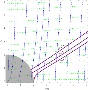
Figure 1: Electromagnetic fields in the vicinity of a Schwarzschild black hole moving in the negative $y$-direction. Shown with blue and green lines are field lines of the magnetic and electric field, respectively, while the horizon is represented as a gray-shaded area. Also shown with thick purple lines are the charge separatrixes $\rho_{\rm ind}=0$ for the different values of the parameter $\beta$ in the plane $\phi=0$. The highest separatrix corresponds to the case $\beta=0.1$, the middle one to the case $\beta=0.6$ and the lowest line to the case $\beta=1$ and these move toward the equatorial plane for growing $\beta$.

Note that in contrast with what happens for Boyer-Linquist coordinates, the electric and magnetic fields have a nonzero covariant $\phi$-component in Kerr-Schild coordinates. Equation (13), in particular, shows that the $\phi$-component of the electric field contains a term which is proportional to $B_{0}$ but not to $\beta$ and which therefore does not vanish when $\beta=0$. This is related to the fact that ZAMO observers also have a radial motion, which is responsible for the appearance of this electric field even if the black hole is not moving; clearly this term vanishes at infinity. An example of the electromagnetic field structure is shown in Fig. 1, where the (green) solid and (blue) dashed vector field lines refer to the electric and magnetic fields, respectively, while the horizon is represented as a gray-shaded area. Note that the electric and magnetic fields are orthogonal only asymptotically and thus that a component of the electric field $\vec{\boldsymbol{E}}_{\parallel}$ parallel to the magnetic field is present near the horizon, which can lead to particle acceleration there (see discussion below).

Also shown with thick purple lines are the charge separatrixes $\rho_{\rm ind}=0$ for the different values of the parameter $\beta$ in the plane $\phi=0$. The highest separatrix corresponds to the case $\beta=0.1$, the middle one to the case $\beta=0.6$ and the lowest line to the case $\beta=1$ and these move toward the equatorial plane for growing $\beta$. This figure should be compared with the corresponding Fig. 1 of Lyutikov (2011), where the electromagnetic fields are however divergent at the horizon and are not reported inside the black hole

Using expressions (11)–(16) we can compute the electromagnetic-field invariants Wald (1974)

$$B^{2}-E^{2}=\frac{1}{2}F_{\mu\nu}F^{\mu\nu}\,,\qquad\boldsymbol{\vec{E}}\cdot\boldsymbol{\vec{B}}=\frac{1}{4}\ ^{*}\!F_{\mu\nu}F^{\mu\nu}\,.$$ (17)

It is then straightforward to define the electric-field component parallel to the magnetic field as

$$\boldsymbol{\vec{E}}_{\parallel}\equiv\frac{\boldsymbol{\vec{E}}\cdot\boldsymbol{\vec{B}}}{B^{2}}\boldsymbol{\vec{B}}\,,$$ (18)

and thus the induced charge density necessary to screen this electric field component is

$$-\rho_{\rm ind}\equiv\frac{1}{4\pi}\nabla\cdot\boldsymbol{\vec{E}}_{\parallel}\,.$$ (19)

The explicit expressions for the invariants $B^{2}-E^{2}$ and $\boldsymbol{\vec{E}}\cdot\boldsymbol{\vec{B}}$, for the parallel electric field $\boldsymbol{\vec{E}}_{\parallel}$ and for the induced charge density $\rho_{\rm ind}$ in Kerr-Schild coordinates have already been reported by Lyutikov Lyutikov (2011), which however are incomplete since they do not include the $\phi$-components of the electric and magnetic fields. The corresponding full expressions are presented in Appendix C [cf. Eq. (95)], while we report below the angular distribution of the induced charge density at first order in the velocity $\beta$.

$$\rho_{\rm ind}(r,\theta)=\frac{E_{0}M\sin\theta\cos\phi}{\pi r^{2}\tilde{N}\left(1+{2M\cos^{2}\theta}/{r}\right)^{2}}\Bigg{(}1-\frac{3}{2}\sin^{2}\theta+\frac{4M}{r}-\frac{5M}{r}\sin^{2}\theta+\frac{4M^{2}}{r^{2}}\cos^{4}\theta+\frac{2M^{2}}{r^{2}}\cos^{2}\theta\sin^{2}\theta\Bigg{)}\,.$$ (20)

Of particular interest in the function (20) is the “separatrix”, namely: the line where the function goes to zero and hence where the charge distribution changes sign. The location of such separatrix is independent of the velocity only when the induced charge distribution is taken at first order in $\beta$ [cf. Eq. (20)]; however, if the complete expression is considered, then the separatrix is a function of the velocity and moves towards the equatorial plane with increasing $\beta$ [cf. Eq. (95)]. This is shown with the thick solid lines in Fig. 1, which refer to velocities $\beta=0.1,0.6,1$, respectively. This effect was not remarked in Lyutikov (2011), where only the first-order expression for the induced charge distribution was considered. Also shown in Fig. 1 are the magnetic-field lines (blue lines) and the electric-field lines (green lines), which tend to be orthogonal at sufficient distances from the black hole horizon.

The following Section will be dedicated to extending the analysis carried out here to the case of a spinning black hole in the Kerr-Schild coordinates.

III Wald solution in Kerr-Schild coordinates

As a warm-up exercise, we re-derive the Wald solution Wald (1974) in Kerr-Schild coordinates and thus for a stationary black hole, as this will be one of the building blocks to obtain the full solution. Following Wald Wald (1974), we exploit the existence in the spacetime (2) of a timelike Killing vector $\xi^{\alpha}_{(t)}$ and of a spacelike one $\xi^{\alpha}_{(\phi)}$, which reflect the stationarity and the axial symmetry of the black hole solution and such that they satisfy the Killing equation

$$\xi_{\alpha;\beta}+\xi_{\beta;\alpha}=0\,.$$ (21)

Following again Wald Wald (1974), we can use Eq. (21) and the tensor identity

$$\xi_{\alpha;\beta;\gamma}-\xi_{\alpha;\gamma;\beta}=-\xi^{\delta}R_{\delta\alpha\beta\gamma}\,,$$ (22)

where $R_{\delta\alpha\beta\gamma}$ is the Riemann curvature tensor, to obtain

$$\Box\xi^{\alpha}=\xi^{\alpha;\beta}_{\ \ \ \ \ ;\beta}=R^{\alpha}_{\ \delta}\xi^{\delta}\,,$$ (23)

where we have permuted cyclically the indices and added the resulting equations after exploiting the symmetries of the Riemann tensor. Because the right-hand side of Eq. (23) vanishes in vacuum, we obtain a wave equation for the Killing vector $\xi^{\alpha}$. Since a Killing vector generates a solution of the Maxwell equations, we set the vector potential to be a linear combination of the Killing vectors

$$A^{\alpha}=C_{2}\xi^{\alpha}_{(t)}+C_{3}\xi^{\alpha}_{(\phi)}\,,$$ (24)

and it is then easy to show that (24) is a solution of the Maxwell equations $F^{\mu\nu}_{\ ;\nu}=0$ and that $\Box A^{\mu}=0$ in the Lorentz gauge $A^{\mu}_{\ ;\mu}=0$ Wald (1974).

Using the ansatz (24), the integration constant $C_{3}$ is found from the requirement that the black hole is immersed into an asymptotically uniform magnetic field, which is parallel to its axis of rotation. This procedure was adopted by Wald in Wald (1974) using Boyer-Lindquist coordinates and of course it can be applied also in the case of Kerr-Schild coordinates. More specifically, once the $z$-component of the magnetic field is evaluated in the orthonormal basis of a ZAMO observer at spatial infinity, it is sufficient to require that this value is equal to $B_{0}$ to obtain the integration constant as $C_{3}=B_{0}/2$.

The remaining integration constant can instead be found after imposing charge neutrality as evaluated through a surface integral across a spherical surface at spatial infinity, i.e.,

$$4\pi Q=0 =\frac{1}{2}\oint F^{\alpha\beta}{{}_{*}dS}_{\alpha\beta}$$

$$=C_{2}\oint\xi_{(t)}^{\alpha;\beta}{{}_{*}dS}_{\alpha\beta}+\frac{B}{2}\oint\xi_{(\phi)}^{\alpha;\beta}{{}_{*}dS}_{\alpha\beta}\,,$$ (25)

where $dS_{\alpha\beta}$ is the infinitesimal element on the 2-sphere. Fortunately, the two integrals in (III) have simple analytic solutions, namely Poisson (2004):

$$\oint\xi_{(t)}^{\alpha;\beta}{{}_{*}dS}_{\alpha\beta}=-8\pi M\,, \oint\xi_{(\phi)}^{\alpha;\beta}{{}_{*}dS}_{\alpha\beta}=16\pi J\,,$$ (26)

so that it is then straightforward to derive that $C_{2}=aB_{0}$.

With the integration constants known, the explicit expressions for the the covariant component of the 4-vector potential $A_{\alpha}$ will take the form

$$A_{t} = -aB_{0}\left(1-\frac{Mr}{\Sigma}(1+\cos^{2}\theta)\right)\,,$$ (27)

$$A_{r} = \frac{aB_{0}}{2}\left(\frac{2Mr}{\Sigma}(1+\cos^{2}\theta)-\sin^{2}\theta\right)\,,$$ (28)

$$A_{\phi} = \frac{B_{0}\sin^{2}\theta}{2\Sigma}\left(A-4Ma^{2}r\right)\,.$$ (29)

Using equations (24) and (27) it is also possible to compute what is the maximum charge that the black hole can support, following the arguments already given in Wald (1974). In particular, it is sufficient to recall that the electrostatic energy of a particle with charge $q_{e}$ in the vicinity of the black hole is simply given by $q_{e}A^{\mu}\xi_{\mu\ (t)}$. Because the Killing vector $\xi_{\mu\ (t)}$ becomes spacelike inside the ergoregion defined by $g_{tt}=0$, it is more convenient to introduce a new Killing vector which is regular at the horizon Carter (1971); Aliev (1993)

$$(\psi_{\mu})_{\rm h}=\xi_{\mu(t)}+\Omega_{\rm h}\xi_{\mu(\phi)}\,,$$ (30)

where

$$(\Omega)_{\rm h}\equiv\frac{a}{2Mr_{+}}\,,\quad r_{+}\equiv M+\sqrt{M^{2}-a^{2}}\,.$$ (31)

The change in the electrostatic energy of the charged particle as it falls from infinity down to the black-hole horizon is thus given by

$$\epsilon =q_{e}\left\{(A^{\mu})_{\rm h}\left[(\xi_{\mu(t)})_{\rm h}+(\Omega)_{\rm h}(\xi_{\mu(\phi)})_{\rm h}\right]-(A^{\mu})_{\rm\infty}(\xi_{\mu(t)})_{\infty}\right\}$$

$$=-q_{e}aB_{0}\,,$$ (32)

where the indices ${\rm h}$ and $\infty$ refer to quantities evaluated at the horizon and at infinity, respectively. Assuming now that the black hole is not electrically neutral, but instead possesses the net electric charge $Q$, Eq. (III) would have to be modified to add for the additional electrostatic contribution induced by the black hole’s charge, i.e.,

$$\epsilon=\frac{q_{e}}{2M}\left(Q-2MaB_{0}\right)\,.$$ (33)

At equilibrium, $\epsilon=0$, so that it is possible to deduce the upper limit for test electric charge as accreted by the rotating black hole as Wald (1974)

$$Q=2aMB_{0}\,.$$ (34)

Clearly, this charge vanishes for a nonrotating black hole.

Collecting things together we deduce that the nonvanishing components of the Faraday tensor are then given by

$$F_{rt} = -\frac{aMB_{0}}{\Sigma^{2}}(r^{2}-a^{2}\cos^{2}\theta)(1+\cos^{2}\theta)\,,$$ (35)

$$F_{\theta t} = -\frac{2aMrB_{0}}{\Sigma^{2}}(r^{2}-a^{2})\sin\theta\cos\theta\,,$$ (36)

$$F_{\theta r} = -aB_{0}\left[\frac{2Mr}{\Sigma^{2}}(r^{2}-a^{2})+1\right]\sin\theta\cos\theta\,,$$ (37)

$$F_{r\phi} = \frac{B_{0}}{\Sigma^{2}}\Bigg{[}2\Sigma r^{3}-Ar+4Ma^{2}r^{2}+a^{2}\Sigma(r-M)(1+\cos^{2}\theta)\Bigg{]}\sin^{2}\theta\,,$$ (38)

$$F_{\theta\phi} = \frac{B_{0}}{\Sigma^{2}}\Bigg{[}(r^{2}+a^{2})(A-4Ma^{2}r)-a^{2}\Delta\Sigma\sin^{2}\theta\Bigg{]}\sin\theta\cos\theta\,.$$ (39)

At this point it is straightforward to compute the expressions for the orthonormal components of the electromagnetic fields measured by the ZAMO observers. Using the four-velocity components (4a)–(4), which are at first order in the spin parameter, the electric field will be given by

$$E^{\hat{r}}=-\frac{aMB_{0}}{\sqrt{A}\Sigma^{3}}\Bigg{\{}\frac{A(r^{2}-a^{2}\cos^{2}\theta)(1+\cos^{2}\theta)}{\left(1+2Mr/\Sigma\right)}-\Bigg{[}2\Sigma r^{4}-Ar^{2}+4Ma^{2}r^{3}+a^{2}r\Sigma(r-M)(1+\cos^{2}\theta)\Bigg{]}\sin^{2}\theta\Bigg{\}}\,,$$ (40)

$$E^{\hat{\theta}}=\frac{2a^{3}MrB_{0}}{\Sigma^{2}\left(\Sigma+2Mr\right)^{1/2}}(1+\cos^{2}\theta)\sin\theta\cos\theta\,,$$ (41)

$$E^{\hat{\phi}}=\frac{2MrB_{0}\sin\theta}{\Sigma^{2}\sqrt{A}\left(\Sigma+2Mr\right)^{1/2}}\Bigg{[}2\Sigma r^{3}-Ar+4Ma^{2}r^{2}+a^{2}\Sigma(r-M)(1+\cos^{2}\theta)\Bigg{]}\,,$$ (42)

while the magnetic field components will be given by

$$B^{\hat{r}}=\frac{2B_{0}\cos\theta}{\Sigma\sqrt{A}\Xi}\Bigg{[}(r^{2}+a^{2})(A-4Ma^{2}r)-a^{2}\Delta\Sigma\sin^{2}\theta\Bigg{]}\,,$$ (43)

$$B^{\hat{\theta}}=-\frac{2B_{0}}{\Sigma\left(\Sigma+2Mr\right)^{1/2}\Xi}\Bigg{[}2\Sigma r^{3}-Ar+4Ma^{2}r^{2}+a^{2}\Sigma(r-M)(1+\cos^{2}\theta)\Bigg{]}\sin\theta\,,$$ (44)

$$B^{\hat{\phi}}=\frac{2aB_{0}\sin\theta\cos\theta}{\sqrt{A}\Sigma^{2}\left(\Sigma+2Mr\right)^{1/2}\Xi}\Bigg{\{}{2MrA}(r^{2}-a^{2})+A-{\left(\Sigma+2Mr\right)}\left[(r^{2}+a^{2})(A-4Ma^{2}r)-a^{2}\Delta\Sigma\sin^{2}\theta\right]\Bigg{\}}\,.$$ (45)

where $\Xi\equiv(a^{2}+2r^{2}+a^{2}\cos 2\theta)$. It is then easy to recognize that the geometric structure of the electric field is complex and with a non trivial dependence from the black-hole’s angular momentum $a$. The radial and polar components of the electric field are due to the dragging of inertial frames and the $\phi$-component is due to the radial fall of ZAMO observer in the Kerr-Schild coordinates. In the limit of a flat spacetime, i.e., for $M/r\rightarrow 0$, and $Ma/r^{2}\rightarrow 0$, expressions (40)–(44) give

$$\lim_{M/r,Ma/r^{2}\rightarrow 0}B^{\hat{r}}=-B_{0}\cos\theta\,,\lim_{M/r,Ma/r^{2}\rightarrow 0}B^{\hat{\theta}}=B_{0}\sin\theta\,,$$

$$\lim_{M/r,Ma/r^{2}\rightarrow 0}B^{\hat{\phi}}=0\,,\qquad\lim_{M/r,Ma/r^{2}\rightarrow 0}E^{\hat{j}}=0\,.$$ (46)

which coincide with the solutions for the homogeneous magnetic field in a Minkowski spacetime. Also, we have checked that the expression (40)–(44) satisfy the Maxwell equations (6a)–(6b).

IV Moving Wald solution in Kerr-Schild coordinates

We next consider the solution of the Maxwell equations for a moving and spinning black hole, thus extending the solutions of Wald and Lyutikov to the most generic case. For simplicity, we will consider the black-hole spin axis to be along the $z$-direction (the same direction of the asymptotically uniform magnetic field) and its velocity to be instead in the negative $y$-direction; more generic configurations can be easily derived but would only introduce additional trigonometric corrections. In addition, to keep the expressions in a compact form, we will consider the black-hole metric in the slow-rotation approximation, that is, at first-order in the spin parameter $a$. In this case, the metric functions (2) reduce to

$$g_{tt} =-N^{2}\,, g_{tr} =g_{rt}=\frac{2M}{r}\,,$$ (47a)

$$g_{t\phi} =g_{\phi t}=-\frac{2Ma\sin^{2}\theta}{r}\,, g_{rr} =1+\frac{2M}{r}\,, \!\!\!g_{\theta\theta} =r^{2}\,,$$ (47b)

$$g_{r\phi} =g_{\phi r}=-a\tilde{N}^{2}\sin^{2}\theta\,, g_{\phi\phi} =r^{2}\sin^{2}\theta\,.$$ (47c)

To obtain the moving Wald solution in Kerr-Schild coordinates, we exploit the linearity of electromagnetic equations and write the solution of Maxwell equations in the spacetime (2) as the superposition of the Wald solution discussed above with the one relative to a moving black hole (7)–(9), so that the covariant components of the vector potential can be written as

$$A_{t} =-aB_{0}\left(N^{2}+\frac{M\sin^{2}\theta}{r}\right)+N^{2}E_{0}r\sin\theta\cos\phi\,,$$ (48a)

$$A_{r} =aB_{0}\left(\frac{2M}{r}-\frac{\tilde{N}^{2}\sin^{2}\theta}{2}\right)-2ME_{0}\sin\theta\cos\phi\,,$$ (48b)

$$A_{\phi} =\frac{B_{0}}{2}r^{2}\sin^{2}\theta\,,$$ (48c)

where we recall that $E_{0}=\beta B_{0}$ is the electric field measured by an observer comoving with the black hole and the axial symmetry is clearly broken through the new dependence on the azimuthal angle $\phi$.

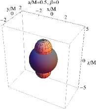
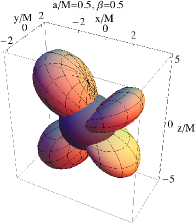
Figure 2: Representative surfaces of the relativistic invariant $\boldsymbol{\vec{E}}\cdot\boldsymbol{\vec{B}}$. More specifically, the different panels show $\boldsymbol{\vec{E}}\cdot\boldsymbol{\vec{B}}=0.1$ for different values of the dimensionless spin parameter $a/M$ and of the black hole dimensioneless speed $\beta$, as reported on the top of each panel. Shown as gray-shaded area is instead the black-hole event horizon.

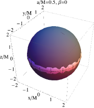
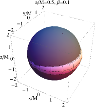
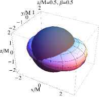
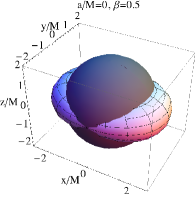
Figure 3: The same as in Fig. 2 but for surfaces at which $|\boldsymbol{\vec{E}}|=|\boldsymbol{\vec{B}}|$.

Using the expressions (48) for the vector potential, we next derive the expressions for the magnetic and electric field as measured by the ZAMO observers for a moving Kerr black hole at first order in the spin. The starting point is the calculation of the nonzero components of the Faraday tensor, which a bit of algebra reveal to be

$$F_{rt} = A_{t,r}=\frac{aB_{0}M}{r^{2}}(\sin^{2}\theta-2)+E_{0}\sin\theta\cos\phi\,,$$ (49)

$$F_{\theta t} = A_{t,\theta}=-\frac{2MaB_{0}}{r}\sin\theta\cos\theta+E_{0}r\tilde{N}^{2}\cos\theta\cos\phi\,,$$

$$F_{\phi t} = A_{t,\phi}-A_{\phi,\,t}=-N^{2}E_{0}r\sin\theta\sin\phi\,,$$ (51)

$$F_{\theta r} = A_{r,\theta}=-\tilde{N}^{2}aB_{0}\sin\theta\cos\theta-2ME_{0}\cos\theta\cos\phi\,,$$

$$F_{r\phi} = A_{\phi,r}=rB_{0}\sin^{2}\theta-2ME_{0}\sin\theta\sin\phi\,,$$

$$F_{\theta\phi} = A_{\phi,\theta}=B_{0}\sin\theta\cos\theta r^{2}\,,$$ (54)

where we have retained terms $\mathcal{O}(a)$ and $\mathcal{O}(\beta)$, neglecting terms $\mathcal{O}(a^{2}),\mathcal{O}(\beta^{2})$ and $\mathcal{O}(a\beta)$.

The physical components of the electric and magnetic fields are again obtained after projecting on the ZAMOs tetrads and are given by

$$B_{\hat{r}}=-B_{0}\cos\theta\,,$$ (55)

$$B_{\hat{\theta}}=\frac{1}{\tilde{N}}\left(B_{0}\sin\theta-\frac{2ME_{0}}{r}\sin\phi\right)\,,$$ (56)

$$B_{\hat{\phi}}=-\frac{2E_{0}M}{r\tilde{N}}\cos\theta\cos\phi\ ,$$ (57)

for the magnetic field (we recall that $E_{0}\equiv\beta B_{0}$) and by

$$E_{\hat{r}}=E_{0}\sin\theta\cos\phi+\frac{aMB_{0}}{r^{2}}(3\sin^{2}\theta-2)\,,$$ (58)

$$E_{\hat{\theta}}=\frac{1}{\tilde{N}}E_{0}\cos\theta\cos\phi\,,\quad$$ (59)

$$E_{\hat{\phi}}=\frac{1}{\tilde{N}}\left(-E_{0}\sin\phi+\frac{2M}{r}B_{0}\sin\theta\right)\,,$$ (60)

for the electric field. Similarly, the expressions for the electromagnetic field invariants $E^{2}-B^{2}$ and $\boldsymbol{\vec{E}}\cdot\boldsymbol{\vec{B}}$ take the form

$$\boldsymbol{\vec{E}}\cdot\boldsymbol{\vec{B}}=\frac{2M}{r}B_{0}\cos\theta\left(E_{0}\sin\theta\cos\phi-\frac{a}{4r}B_{0}(1+3\cos 2\theta)\right)\,,$$ (61)

$$B^{2}-E^{2}=B_{0}^{2}\Bigg{\{} (1-\beta^{2})+\frac{2M}{r}\left[\beta^{2}(\cos^{2}\theta\cos^{2}\phi+\sin^{2}\phi)-\sin^{2}\theta\right]+\frac{a\beta M}{2r^{2}}\left(3\sin 3\theta-\sin\theta\right)\cos\phi$$

$$+\frac{a^{2}}{4r^{2}}\left[2(\cos 2\theta-1)+\frac{M}{r}(\cos 4\theta-1)+\frac{M^{2}}{2r^{2}}(1-28\cos 2\theta-5\cos 4\theta)\right]\Bigg{\}}\ ,$$ (62)

while the expressions for the parallel electric field $\boldsymbol{\vec{E}}_{\parallel}$ and for the charge density $\rho_{\rm ind}$ can be calculated to be respectively

$$E_{\parallel}=\frac{\tilde{N}M}{r\sqrt{1+{2M}/{r}\cos^{2}\theta}}\Bigg{[}2E_{0}\sin\theta\cos\theta\cos\phi-\frac{a}{2r}B_{0}\cos\theta(1+3\cos 2\theta)\Bigg{]}\,,$$ (63)

and

$$\rho_{\rm ind}=\frac{B_{0}M}{32\pi r^{3}\tilde{N}\left(1+{2M\cos^{2}\theta}/{r}\right)^{2}} \Bigg{\{}8\beta r\cos\phi\sin\theta\Bigg{[}1+\frac{7M^{2}}{r^{2}}+\frac{6M}{r}$$

$$\hskip-85.35826pt+\left(\frac{2M}{r}+1\right)\left(\frac{4M}{r}+3\right)\cos 2\theta+\frac{M^{2}}{r^{2}}\cos 4\theta\Bigg{]}-a\Bigg{[}5+\frac{24M}{r}+\frac{26M^{2}}{r^{2}}$$

$$+\left(\frac{5M}{r}+3\right)\left(\frac{11M}{r}+4\right)\cos 2\theta +\left(\frac{38M^{2}}{r^{2}}+\frac{48M}{r}+15\right)\cos 4\theta+\frac{3M}{r}\left(\frac{3M}{r}+1\right)\cos 6\theta\Bigg{]}\Bigg{\}}\,.$$ (64)

Note that in addition to the lowest-order terms, the invariant $B^{2}-E^{2}$ also contains terms $\mathcal{O}(a^{2})$, and $\mathcal{O}(\beta^{2})$, since no terms $\mathcal{O}(a)$, or $\mathcal{O}(\beta)$ are present.

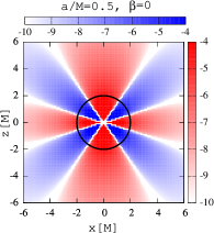
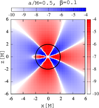
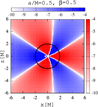
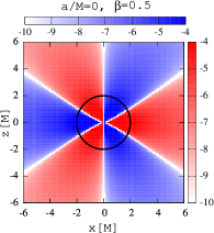
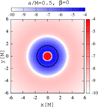
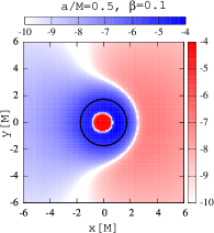
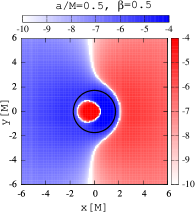
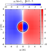
Figure 4: Induced charge-density distribution $\rho_{\rm ind}$ for $M=1$, $B_{0}=1$, and different values of $a/M$ and $\beta$. The charge distribution is indicated with a colorscale in which blue refers to positive charges and red to negative charges, respectively. The upper row refers to a projection in the $(x,z)$ plane with a logarithmic colorscale, while the bottom one to a projection in $(x,y)$ plane at $z/M=1$. Indicated with a solid black circles are the black hole horizons. Regions in white correspond to zero induced charges and thus separate two domains with opposite charges.

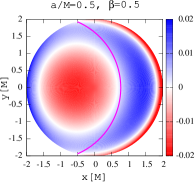
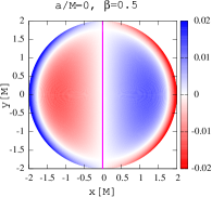
Figure 5: Projection on the $(x,y)$ plane of the induced charge-density distribution on the event horizon. The colormaps are the same as in Fig. 4 but shown with a linear colorscale to highlight the small-scale variations. The two panels refer to the last two columns in Fig. 4 and we have indicated with magenta solid line separatrixes $E_{\parallel}=0$.

Figure 2 shows representative surfaces of the relativistic invariant $\boldsymbol{\vec{E}}\cdot\boldsymbol{\vec{B}}$ and, more specifically, the surface $\boldsymbol{\vec{E}}\cdot\boldsymbol{\vec{B}}=0.1$. The different panels refer to different values of the spin parameter $a/M$ and of the black hole velocity $\beta$, as reported on the top of each panel. Shown instead as gray-shaded area is the black-hole event horizon, which is located at $2M$ [the true position of the horizon is of course $r=M+\sqrt{M^{2}-a^{2}}\simeq 2M+\mathcal{O}(a^{2})$]. Note that although the axial symmetry is broken by the presence of a velocity, reflection symmetries are still present with respect to the $(x,z)$ plane and to the $(x,y)$ plane. Similarly, Fig. 3 shows the position of the surfaces at which $|\boldsymbol{\vec{E}}|=|\boldsymbol{\vec{B}}|$ for the same values of the parameters $a/M$ and $\beta$ selected in Fig. 2. Note that the reflection symmetry across the $(y,z)$ plane is lost as soon as the black hole is rotating (i.e., for $a\neq 0$), but that the reflection symmetries with respect to the $(x,z)$ and $(x,y)$ planes remain.

Finally, in Fig. 4 we show the induced charge density $\rho_{\rm ind}$ for the same set of parameters $a/M$ and $\beta$ used in the previous two figures. More specifically, the upper row refers to a projection in the $(x,z)$ plane and where we have indicated with a solid black line the black-hole horizon. The bottom row is the same as the top one but with a projection in $(x,y)$ plane and we have indicated with a magenta solid line the separatrix $E_{\parallel}=0$. Note that in all panels the areas in white correspond to regions with zero induced charges and thus separate two domains with opposite charges (we have indicated with blue regions of positive charges and with red regions of negative charges). Note also that the velocity-induced corrections are generically the most important ones, with the charge density assuming its maximum values in the equatorial plane and that the spin-induced corrections are evident only for comparatively small values of the velocity (cf. the first two panels of Fig. 4. Finally, we note that the use of the Kerr-Schild coordinates allows us to have a complete and regular description of the charge distribution even inside the event horizon, in contrast with the results of Lyutikov (2011), where the distribution was singular at the horizon. This is highlighted in Fig. 5, which shows a magnification of the projections on the $(x,y)$ plane of the induced charge-density distribution on the event horizon. The colormaps are the same as in Fig. 4 but shown with a linear colorscale to highlight the small-scale variations. The two panels refer to the last two columns in Fig. 4 and we have indicated with magenta solid line separatrixes $E_{\parallel}=0$. An additional discussion of this figure will be made also in the following Section.

V electromagnetic energy losses

In the scenario considered here, all of the magnetic field lines threading the horizon of the moving and rotating black hole are connected to infinity. Under these conditions, winds of charged particles can be produced and flow along the magnetic field lines, being accelerated by the electric-field components parallel to the magnetic-field lines. The origin of the particles in the wind is still a matter of debate, but as discussed in Ref. Lyutikov (2011), it is possible that the potential gap in the vicinity of the black hole is large enough for the creation of particles due to electron-positron cascades. Alternatively, any stray charged particle orbiting near the black hole could be accelerated to high Lorentz factors by the large electric fields and thus be able to produce pairs.

If the acceleration of charged particles and a cascade via pair generation takes place in the vicinity of the black hole, it may build up a plasma magnetosphere. Obviously, the charge density and the velocity distribution of the magnetospheric plasma cannot be described accurately within our approach, but we can exploit the analogies with the physics of pulsar magnetosphere. We can therefore estimate $\rho_{\rm ind}$ as the induced charge density needed in order to screen the parallel component of electric field. Furthermore, assuming that the charged particles are rapidly accelerated up to relativistic velocities, we can take as modulus of the current density in the black hole magnetosphere the upper limit $c\rho_{\rm ind}$. These estimates are clearly very crude and analogous to those made in Ref. Lyutikov (2011), but are useful as they provide us with a bulk reference current through which we can estimate the electromagnetic energy losses within the membrane paradigm Crowley et al. (1986). As we will discuss later on, a comparison with numerical-relativity calculations shows that the error associated to this approximation is only of a factor of a few.

We recall that the membrane paradigm of black-holes electrodynamics represents an elegant and very useful approach in which relativistic black-hole electrodynamics resembles classical electrodynamics Crowley et al. (1986). In particular, the membrane paradigm considers the extended horizon of the black hole as a conducting sphere which is endowed with physical properties, such as a surface resistivity, a surface charge and a current density. Although this is only an effective construction, the membrane paradigm serves as a useful physical guideline, providing the interpretation of the complex phenomena taking place in the vicinity of black holes (see Penna et al. (2013) for a recent comparison between the membrane-paradigm description of the Blandford-Znajek mechanism and the results of general-relativistic magnetohydrodynamical simulations).

In order to estimate the electromagnetic energy losses it is important to know the distribution of the charges and currents in and out of the black-hole magnetosphere and, in particular, the location of the surfaces where $E_{\parallel}=0$ or $\rho_{\rm ind}=0$. These surfaces, in fact, divide the space in domains where electric currents of different sign are nonzero and of variable intensity. As a result, the two-dimensional surfaces with $E_{\parallel}=0$ and $\rho_{\rm ind}=0$ mark the separation between regions with currents in different directions and charges of opposite signs, respectively. Such surfaces are simply obtained from Eqs. (63) and (IV) and thus described by the following equations

$$4\beta r\sin\theta\cos\phi-{a}(1+3\cos 2\theta)=0\,,\qquad\cos\theta=0\,,$$ (65)

and

$$8\beta r\cos\phi\sin\theta\Bigg{[}1+\frac{7M^{2}}{r^{2}}+\frac{6M}{r}+\left(\frac{2M}{r}+1\right)\left(\frac{4M}{r}+3\right)\cos 2\theta+\frac{M^{2}}{r^{2}}\cos 4\theta\Bigg{]}-a\Bigg{[}5+\frac{24M}{r}+\frac{26M^{2}}{r^{2}}$$

$$\quad+\left(\frac{5M}{r}+3\right)\left(\frac{11M}{r}+4\right)\cos 2\theta+\left(\frac{38M^{2}}{r^{2}}+\frac{48M}{r}+15\right)\cos 4\theta+\frac{3M}{r}\left(\frac{3M}{r}+1\right)\cos 6\theta\Bigg{]}=0\,.$$ (66)

In the limiting case when $a=0,\ \beta\neq 0$, the first of Eqs. (65) divides the space into four quadrants, while the second one simply marks the equatorial plane (i.e., $\cos\theta=0$); similarly, when $a\neq 0,\ \beta=0$, the first of Eqs. (65) marks conical surfaces in the upper and lower hemispheres (i.e., $1+3\cos 2\theta=0$). In the more general case of nonzero values for $a$ and $\beta$, the surface with $E_{\parallel}=0$ is rather complex, but it represents, overall, the transition between these two limiting cases. It should be noted that the different scaling with radius of the spin-induced contributions (that decrease like $1/r^{3}$) and of the velocity-induced contributions (that decrease like $1/r^{2}$) is such that the former are important only in the vicinity of the black hole. At large distances, therefore, the shape of the separating surfaces will be quite similar to the case of nonrotating black holes discussed in Ref. Lyutikov (2011).

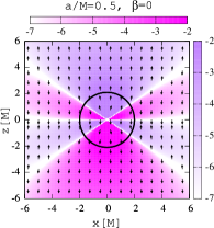
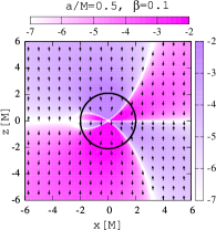
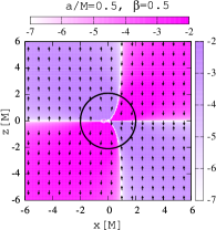
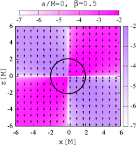
Figure 6: Electric-field component parallel to the magnetic field, $E_{\parallel}$ in the $(x,z)$ plane. The arrows show the direction of the field lines, while the solid black circle marks the position of the horizon. Violet colors show the regions where the considered component of the electric field is directed along the magnetic field lines, while the magenta colors show the opposite.

Figure 6 reports the electric field $E_{\parallel}$ in the $(x,z)$ plane and for the same values of the parameters $a$ and $\beta$ used in the previous figures. More specifically, the arrows show the direction of the parallel electric field lines, while the black solid line marks the position of the horizon. Violet colors refer to regions where the electric field is in the same direction as the magnetic field lines, while the magenta colors show the opposite; in either case, the reported colormaps can be used to deduce the strength of the field. As remarked for the induced charge density, also the induced parallel electric field is most sensitive to the velocity of the black hole and the qualitative features of the solution do not change appreciably for $\beta\gtrsim 0.5$. This is more evident for the electric field distribution in the $(y,z)$ plane, which is shown in Fig. 7, and where we report only the solutions corresponding to the last two panels of Fig. 6; these field structures are essentially insensitive to further increases in the velocity.

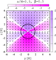
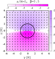
Figure 7: The same as in Fig. 6, but for the electric field in the $(y,z)$ plane. Note that we report only the solutions corresponding to the last two panels of Fig. 6, as these are the most representative ones, with the solution in this plane being essentially insensitive to changes in the velocity.

We should note that when considering the $x=0$ plane, i.e., for $\phi=\pi/2$, the first of Eqs. (65) loses its dependence on $\beta$ and thus the position of the separating surfaces $E_{\parallel}=0$ in this plane remains the same as in the left panel of Fig. 7 for any nonzero $a$ and any $\beta$. Furthermore, when $a=0$, the $x=0$ plane contains the separatrix and thus $E_{\parallel}=0$ on this plane. In order to show a nonzero parallel field, the right panel of Fig. 7 refers to a $(y,z)$ plane at $x=0.3\,M$.

For arbitrary values of $a$ and $\beta$, the position of the separatrixes will be such that each hemisphere will be divided on four domains with different directions of the electric currents. In order to estimate the energy losses within a membrane-paradigm approach, it is necessary to have the values of the currents close to the horizon. In contrast with Ref. Lyutikov (2011), this is not problematic to do here, since our use of Kerr-Schild coordinates implies that we can consider and integrate necessary quantities directly at the horizon, as none of the equations discussed in the previous sections is singular there. In particular, at the horizon the induced charge density is equal to

$$\rho_{\rm ind}=\frac{B_{0}}{32\sqrt{2}\pi M}\frac{1}{(1+\cos^{2}\theta)^{2}}\Bigg{[}4\beta\cos\phi\sin\theta\left(\cos^{4}\theta+9\cos^{2}\theta-2\right)-\frac{a}{M}\left(15\cos^{6}\theta+26\cos^{4}\theta-27\cos^{2}\theta+2\right)\Bigg{]}\,,$$

and the separatrixes are given by

$$\sin\theta=-\frac{{2\beta M}\cos\phi-\sqrt{{4\beta^{2}M^{2}}\cos^{2}\phi+6{a^{2}}}}{3{a}}\,,$$ (68)

and

$$15a\sin^{6}\theta + 4\beta M\cos\phi\sin^{5}\theta-71a\sin^{4}\theta$$

$$\hskip-42.67912pt-44\beta M\cos\phi\sin^{3}\theta+70a\sin^{2}\theta$$

$$\hskip-14.22636pt+32\beta M\cos\phi\sin\theta-16a=0\,.$$

Some examples of the position of separatrixes on the black-hole horizon as projected on the $(x,y)$ plane are presented in Fig. 5. The separatrixes for the induced charge density are indicated with white, while magenta lines indicate the position of the separatrix $E_{\parallel}=0$. Note that in the left panel of Fig. 5, one of the separatrixes for $\rho_{\rm ind}$ intersects the equatorial plane at the values of $\phi\sim\pi/2$ and $\phi\sim 3\pi/2$. These points correspond to the solution of Eq. (V) when $\theta=\pi/2$ and thus satisfy the condition

$$\cos\phi=-\frac{a}{4\beta M}\,.$$ (70)

Equation (70) has two distinct solutions only for $\beta\geq a/4M$; for velocities that are instead $\beta<a/4M$, a separatrix for the charge density $\rho_{\rm ind}$ still exists but is not contained in the equatorial plane. As can be seen from Eq. (68), and in the left panel of Fig. 5, the separatrix $E_{\parallel}=0$ intersects the equatorial plane in the same points.

Let us now go back to the calculation of the luminosity by taking the integral of the current density $c\rho_{\rm ind}$ at the horizon [see also Eq. (25) of Lyutikov (2011)]

$$I=(2M)^{2}\int_{\phi_{1}}^{\phi_{2}}d\phi\int_{\theta_{1}}^{\theta_{2}}\rho_{\rm ind}\sin\theta d\theta\,,$$ (71)

to find the current that flows within each domain restricted by the surfaces with $E_{\parallel}=0$ and $\rho_{\rm ind}=0$, with $\phi_{1,2}$ and $\theta_{1,2}$ describing the boundaries of these domains. A schematic diagram illustrating the different integration domains as projected in the $(x,y)$ plane is shown in Fig. 8, where the rotating black hole has the spin along the positive $z$ direction and is moving in the negative $y$-direction.

Interestingly, the integration in the $\theta$-direction can be taken analytically to obtain the expression

$$I=\frac{B_{0}M}{8\sqrt{2}\pi}\Bigg{\{} 2\beta\int_{0}^{2\pi}d\phi\cos\phi\left[-14\theta+\frac{\sin\theta\cos\theta(9-\cos^{2}\theta)}{1+\cos^{2}\theta}-\frac{18}{\sqrt{2}}\arctan(\sqrt{2}\cot\theta)\right]\Bigg{|}_{\theta_{1}}^{\theta_{2}}+$$

$$\frac{a}{M}\int_{0}^{2\pi}d\phi\left[\frac{\cos\theta(5\cos^{4}\theta+\cos^{2}\theta+16)}{1+\cos^{2}\theta}-14\arctan\cos\theta\right]\Bigg{|}_{\theta_{1}}^{\theta_{2}}\Bigg{\}}\,.$$ (72)

This equation extends Eq. (25) of Ref. Lyutikov (2011) to the case of a black hole that is also spinning. It should be noted, however, that in Eq. (25) of Lyutikov (2011), the integration is performed only in the quadrant restricted by the condition $E_{\parallel}=0$ and that the separatrixes for the induced charge density $\rho_{\rm ind}$ are neglected. Equation (V), on the other hand, takes into account both signs of the parallel electric field $E_{\parallel}$ and the induced charge density $\rho_{\rm ind}$.

The integration of (V) in the $\phi$-direction can only be achieved numerically to obtain the values of the four currents, $I_{1}$, $I_{2}$, $I_{3}$ and $I_{4}$ flowing in four domains of the upper hemisphere (cf. Fig. 8). Adopting now the physical description proposed in the membrane paradigm Crowley et al. (1986), the surface resistivity of a black-hole horizon is $\sim 4\pi$, so that we can estimate that each of the four currents $I_{j}$ with $j=1,\ldots 4$, will be responsible for electromagnetic energy losses of the order of $4\pi I_{j}^{2}$. Summing these contributions we readily obtain the electromagnetic losses as a function of the spin parameter and black-hole velocity, i.e.,

$$L_{{}_{\rm EM}}=L_{{}_{\rm EM}}(a;\beta)=8\pi\sum_{j=1}^{4}|I_{j}|^{2}\,,$$ (73)

where additional factor $2$ is the result of the symmetry between upper and lower hemispheres.

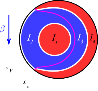
Figure 8: Schematic diagram illustrating the different integration domains as projected in the $(x,y)$ plane and needed to compute expression (V). We recall that the domains reported in the figure refer to a rotating black hole with spin in the positive $z$ direction and moving in the negative $y$-direction.

To fix ideas and after considering a reference magnetic field $B=10^{4}\,{\rm G}$, we report below the estimates for the electromagnetic losses relative to some representative cases, e.g., for a non-spinning but moving black hole

$$L_{{}_{\rm EM}}(0;\beta)=7.2\times 10^{44}\,\beta^{2}\left(\frac{B}{10^{4}\,\mathrm{G}}\right)^{2}\!\!\left(\frac{M}{10^{8}\,M_{\odot}}\right)^{2}\!\!\mathrm{erg\ s^{-1}}\,,\\$$ (74)

or for a stationary but rotating black hole

$$L_{{}_{\rm EM}}(a;0)=2.4\times 10^{44}\,\frac{a^{2}}{M^{2}}\left(\frac{M}{10^{8}\,M_{\odot}}\right)^{2}\!\!\left(\frac{B}{10^{4}\,\mathrm{G}}\right)^{2}\!\!\mathrm{erg\ s^{-1}}\,,\\$$ (75)

or for the more generic case of a black hole with $a=M/2$ and $\beta=0.4$

$$L_{{}_{\rm EM}}(0.5;\,0.4)=1.9\times 10^{44}\,\left(\frac{B}{10^{4}\,\mathrm{G}}\right)^{2}\!\!\left(\frac{M}{10^{8}\,M_{\odot}}\right)^{2}\!\!\mathrm{erg\ s^{-1}}\,.\\$$ (76)

By comparing expressions (74)–(76) it is quite clear that the order-of-magnitude estimate of the luminosity $\sim 10^{44}\,\mathrm{erg\ s^{-1}}$ is rather robust and does not depend sensitively on the specific values of $a/M$ and $\beta$. The general behaviour of the electromagnetic losses as a function of spin and velocity is shown in Fig. 9, which reports the logarithm of the luminosity (73) for different values of $a/M$ and $\beta$; clearly, because of the perturbative nature of our approach, the estimates for $a/M\simeq 1$ and $\beta\simeq 1$ should be taken as indicative only.

It should be noted that for a system with equal values of $\beta$ and $a$ (as it is possible, for instance, in the case of black-hole binaries), the contribution of the linear velocity will be larger than that of the angular momentum. This may be explained intuitively if one assumes that both in the case of a spinning black hole and of a moving one what is relevant is the relative velocity between the magnetic field lines and the horizon. Under this assumption, it is easy to realize that even for maximally rotating black holes, the linear velocity of the horizon is far smaller than the speed of light and hence the spin-induced contributions are at most a fraction of those coming from the linear motion. A similar conclusion, namely that linearly moving black holes lose more energy than spinning ones, was also reached in Ref. Neilsen et al. (2011), where numerical-relativity calculations were carried out for moving and spinning black holes in a force-free plasma. Of course, from an astrophysical point of view it is probably easier to produce black holes that are close to being maximally spinning than black holes that are moving near the speed of light.

As a validation of the robustness of the estimates in expressions (74)–(76), we can compare them with the electromagnetic losses derived in terms of the Poynting flux computed from numerical simulations of the merger of binary black holes in a force free plasma Palenzuela et al. (2010b); Alic et al. (2012). Of course, this comparison should be taken with some care, since expression (73) for the energy losses is obtained using the expression for the induced charge density which, in turn, is derived from the electrovacuum solutions for the electromagnetic fields (55) and (58). The presence of a plasma magnetosphere, as the one emerging from the numerical simulations, changes the structure of the electromagnetic fields around the black hole as the currents generated by the charged particles will create additional components of the magnetic and electric fields, possibly screening the component of the electric field parallel to the magnetic one. Bearing this in mind and assuming that the energy losses from the binary system of black holes to be a sum of the losses from the individual black holes, it is interesting to note that the estimate in (76) is only a factor three larger than the one computed in Ref. Alic et al. (2012) during the inspiral of binary system of black-hole within a force-free plasma; a similar but slightly worse agreement is obtained also when comparing with the results in Ref. Palenzuela et al. (2010b). This agreement is of course reassuring, but is mostly the result of the fact that our luminosity estimate (76) has the right scaling properties with mass and magnetic field, rather than the same level of accuracy of the numerical simulations.

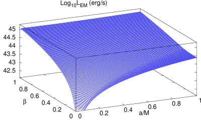
Figure 9: Logarithm of the electromagnetic energy losses from the rotating and linearly moving black hole immersed into the asymptotically uniform magnetic field, estimated as (73), for the different values of $a$ and $\beta$.

VI Conclusions

We have derived analytic solutions for the structure of test electromagnetic fields in the vicinity of a rotating black hole that is also moving at constant speed with respect to an asymptotically uniform magnetic field aligned with the black-hole spin. In practice, this represents the extension to a moving black hole of the classical solution found in 1974 by Wald Wald (1974) for a spinning black hole in a uniform magnetic field. In order to avoid singularities at the black-hole horizon we have employed Kerr-Schild coordinates instead of the Boyer-Lindquist coordinates that have been adopted in recent and related work Lyutikov (2011).

Overall, the electromagnetic fields found can be seen as the linear combination of a contribution coming from the translational motion of black hole relative to the magnetic field, together with a contribution coming from the black-hole rotation and thus ultimately from the dragging of inertial frames in the Kerr spacetime. These latter contributions decay more rapidly with the distance from the black hole than those due to the black-hole velocity. As a result, at large distances from the black hole, the structure of the electromagnetic fields, i.e., the component of the electric field parallel to the magnetic field and the induced charge density necessary to screen this component, are rather similar to those described in Ref. Lyutikov (2011), where a moving Schwarzschild black hole was considered.

After adopting a membrane-paradigm description of the electrodynamics of moving and spinning black holes Crowley et al. (1986), we could estimate the electromagnetic energy losses by computing the currents that would develop on the black-hole horizon as a function of its spin and velocity. Our choice of coordinates was particularly useful for this task, as none of the electromagnetic fields that we have derived is singular at the horizon, in contrast with what would happen if more standard Boyer-Lindquist coordinates were used Lyutikov (2011). Not surprisingly, we find that the electromagnetic losses depend quadratically on the black-hole dimensionless spin $a/M$ and on the velocity velocity $\beta$. However, we find that the energy losses due to the spin are considerably smaller than those due to the translational motion; this is in qualitative agreement with the conclusions reached in Ref. Neilsen et al. (2011), who carried out numerical-relativity calculations of moving and spinning black holes in a force-free plasma.

All things considered, an order-of-magnitude estimate for the electromagnetic luminosity that would be produced by such an object is $L_{{}_{\rm EM}}\sim 10^{44}\ \mathrm{erg\ s^{-1}}$, and this seems to be rather robust and does not depend sensitively on the specific values of $a/M$ and $\beta$. Interestingly, this estimate is only a factor three larger than the one computed during the inspiral of a binary system of black holes in the force-free approximation Palenzuela et al. (2010b); Alic et al. (2012). This agreement is mostly due to the correct scaling of our estimate with mass and magnetic field, but it highlights that analytic and more idealized modelling of the electrodynamics of rotating black holes in magnetic fields can be useful approach to model, at least qualitatively, much more complex and realistic scenarios.

Appendix A Maxwell equations for a black hole moving in a magnetic field

In the following we sketch the procedure we have followed to derive the solutions of the Maxwell equations for a black hole moving in a magnetic field. We start by considering a spherical polar coordinate system $(t,r,\theta,\phi)$ in which we rewrite the Schwarzschild metric as

$$ds^{2}=-N^{2}dt^{2}+N^{-2}dr^{2}+r^{2}(d\theta^{2}+\sin^{2}\theta d\phi^{2})\,.$$ (77)

In such a background spacetime, the vacuum Maxwell equations (6a)–(6b) become

$$\hskip-14.22636ptN^{2}\frac{\partial}{\partial r}\left(r^{2}\frac{\partial}{\partial r}A_{t}\right)+\frac{1}{\sin\theta^{\prime}}\frac{\partial}{\partial\theta^{\prime}}\left(\sin\theta^{\prime}\frac{\partial}{\partial\theta^{\prime}}A_{t}\right)=0\,,~{}~{}$$ (78)

$$\hskip-14.22636ptr^{2}\frac{\partial}{\partial r}\left(N^{2}\frac{\partial}{\partial r}A_{\phi}\right)+\sin\theta\frac{\partial}{\partial\theta}\left(\frac{1}{\sin\theta}\frac{\partial}{\partial\theta}A_{\phi}\right)=0\,,$$ (79)

where $\theta^{\prime}$ and $\theta$ are angles with respect to the axes aligned with the electric and magnetic fields at infinity (see Lyutikov (2011) for a discussion). Following  Beskin (2009), we look for the solution of the Eq. (79) in the form

$$A_{\phi}=\sum_{m=0}^{\infty}g_{m}(r)Q_{m}(\theta)\,,$$ (80)

where $Q_{m}(\theta)$ are the eigenfunctions of the operator

$$\hat{\mathcal{L}}_{\theta}=\sin\theta\frac{\partial}{\partial\theta}\left(\frac{1}{\sin\theta}\frac{\partial}{\partial\theta}\right)\,,$$ (81)

and the equation for the radial eigenfunctions $g_{m}(r)$ has the form

$$x(x-1)\frac{d^{2}g_{m}}{dx^{2}}+\frac{dg_{m}}{dx}-m(m+1)g_{m}=0\,,$$ (82)

where $x\equiv r/2M$. As argued in Ref. Beskin (2009), the physical solution of the equation (79) corresponding to a magnetic field $B_{0}$ that is uniform at the infinity is given by $g_{m}(x)=x^{2}\mathcal{F}(1-m,\ m+2;\ 3;\ x)$, where $\mathcal{F}(a,\ b;\ c;\ x)$ is the hypergeometric function of the argument $x$ with the generic parameters $a,\ b,\ c$. In the case of $m=1$, the $\phi$-component of the vector potential has the simple expressions

$$A_{\phi}=\frac{B_{0}}{2}r^{2}\sin^{2}\theta\,,\quad A^{\phi}=\frac{B_{0}}{2}\,.$$ (83)

On the other hand, the solution to Eq. (78) can be found assuming the ansatz

$$A_{t}=h(r)f(\theta)\,,$$ (84)

where the functions $h(r)$ and $f(\theta)$ are given by the equations

$$\left(1-\frac{2M}{r}\right)\frac{1}{h}\frac{d}{dr}\left(r^{2}\frac{dh}{dr}\right) = K\,,$$

$$\frac{1}{\sin\theta}\frac{1}{f}\frac{d}{d\theta}\left(\sin\theta\frac{df}{d\theta}\right) = -K\,,$$ (85)

with $K$ an integration constant. A physical solution of Eq. (78) describing an electric field $E_{0}$ that is uniform at infinity corresponds to the case $K=2$, $h(r)=C_{1}(r-2M)$ and $f(\theta)=P_{1}(\cos\theta^{\prime})=\cos\theta^{\prime}$, where $P_{n}(\theta)$ is the Legendre polynomial of order $n$. Adjusting the constant $C_{1}$ to obtain the value of the electric field at infinity to be $E_{0}$, it is possible to obtain the expression for the $t$-component of the vector potential as

$$A_{t}=E_{0}rN^{2}\cos\theta^{\prime}\,,\quad A^{t}=-E_{0}r\cos\theta^{\prime}\,.$$ (86)

These considerations have been made for a set of spherical polar coordinates to the which, for instance, the Boyer-Lindquist coordinates tend to at large distances. To obtain instead the components of the vector potential $A^{\mu}$ in Kerr-Schild coordinates it is necessary to use the transformation matrix between the two coordinate systems. Calculating the components of the transformation matrix is tedious but straightforward, especially if one bears in mind that that the coordinates $r$ and $\theta$ are the same in the Boyer-Lindquist (BL) and Kerr-Schild coordinate systems (KS), i.e.,

$$r[\sf{KS}]=r[\sf{BL}]\,,\qquad\qquad\theta[\sf{KS}]=\theta[\sf{BL}]\,,$$ (87)

so that the corresponding diagonal components are equal to one. Indeed, all of the diagonal components of the transformation matrix are equal to one. On the other hand, the only nonzero off-diagonal components are (see, e.g.,  Komissarov (2004))

$$\frac{\partial t[\sf{KS}]}{\partial r[\sf{BL}]}=\frac{2Mr}{\Delta}\,,\qquad\quad\frac{\partial\phi[\sf{KS}]}{\partial r[\sf{BL}]}=\frac{a}{\Delta}\,.$$ (88)

Because of the identities (87), the components of the vector potential $A^{t}$ and $A^{\phi}$ from equations (83) and (86) in Boyer-Lindquist coordinates are the same also in Kerr-Schild coordinates. On the other hand, the components $A_{\mu}$ in the Kerr-Schild coordinates may be obtained from them lowering indexes with the help of the metric (2) when $a=0$.

When the black hole is moving in the negative $y$-direction and orthogonally to the uniform magnetic field in the $z$-direction, a comoving observer will measure an electric field which is uniform at infinity and directed along the $x$-axis. The angle $\theta^{\prime}$ in Eqs. (78) and (86) represents the polar angle with respect to the asymptotic electric field (i.e., the $x$-axis in our case). To transform the expressions to the polar spherical coordinate system used in the rest of the paper and in which the polar axis is along the asymptotic magnetic field, one needs to apply the transformation $\cos\theta^{\prime}=\sin\theta\cos\phi$, resulting in Eq. (7) (see also the discussion in Ref. Lyutikov (2011)).

Appendix B Dual transformation of the vacuum Maxwell equations

Following Lyutikov (2011), it is easy to show that electric and magnetic fields given respectively by expressions (11)–(13) and (14)–(16) have the identical structure. To demonstrate this, we start from (11)–(13) and find the corresponding components of the electric field in the Cartesian system of coordinates

$$\begin{bmatrix}E_{\hat{x}}\\ E_{\hat{y}}\\ E_{\hat{z}}\end{bmatrix}=\begin{bmatrix}\sin\theta\cos\phi&\cos\theta\cos\phi&-\sin\phi\\ \sin\theta\sin\phi&\cos\theta\sin\phi&\cos\phi\\ \cos\theta&-\sin\theta&0\end{bmatrix}\begin{bmatrix}E_{\hat{r}}\\ E_{\hat{\theta}}\\ E_{\hat{\phi}}\end{bmatrix}\,.$$ (89)

Now we can introduce another Cartesian system of coordinates $(x^{\prime},y^{\prime},z^{\prime})$ such that $-\hat{x}\rightarrow\hat{z}^{\prime}$, $\hat{z}\rightarrow\hat{x}^{\prime}$, $\hat{y}\rightarrow\hat{y}^{\prime}$, and associate with it a spherical system of coordinates $(r^{\prime},\theta^{\prime},\phi^{\prime})$ with $r^{\prime}=r$. It follows that the following relations hold between the angles

$$\cos\theta^{\prime} = -\sin\theta\cos\phi\,,$$

$$\sin\theta^{\prime}\cos\phi^{\prime} = \cos\theta\,,$$

$$\sin\theta^{\prime}\sin\phi^{\prime} = \sin\theta\sin\phi\,,$$

while the components of the electric field satisfy

$$E_{\hat{x}^{\prime}} = E_{\hat{z}}\,,$$

$$E_{\hat{y}^{\prime}} = E_{\hat{y}}\,,$$ (90)

$$E_{\hat{z}^{\prime}} = -E_{\hat{x}}\,.$$

Performing now the transformation to the “primed” spherical coordinates

$$\begin{bmatrix}E_{\hat{r}^{\prime}}\\ E_{\hat{\theta}^{\prime}}\\ E_{\hat{\phi}^{\prime}}\end{bmatrix} = \begin{bmatrix}\sin\theta^{\prime}\cos\phi^{\prime}&\sin\theta^{\prime}\cos\phi^{\prime}&\cos\theta^{\prime}\\ \cos\theta^{\prime}\cos\phi^{\prime}&\cos\theta^{\prime}\sin\phi^{\prime}&-\sin\theta^{\prime}\\ -\sin\phi^{\prime}&\cos\phi^{\prime}&0\end{bmatrix}\begin{bmatrix}E_{\hat{x}^{\prime}}\\ E_{\hat{y}^{\prime}}\\ E_{\hat{z}^{\prime}}\end{bmatrix}\,,$$

we obtain

$$E_{\hat{r}^{\prime}} = -E_{0}\cos\theta^{\prime}$$ (92)

$$E_{\hat{\theta}^{\prime}} = {\tilde{N}}^{-1}\left[E_{0}\sin\theta^{\prime}-({2M}/{r})B_{0}\sin\phi^{\prime}\right]$$ (93)

$$E_{\hat{\phi}^{\prime}} = -({2M}/{r\tilde{N}})B_{0}\cos\theta^{\prime}\cos\phi^{\prime}$$ (94)

Comparing these components with expressions (14)–(16) for the magnetic field, it is clear that the electric field has the same structure with respect to the $x$-axis as the magnetic field with respect to the $z$-axis. Thus, as remarked in the footnote 2, the dual solution to (11)–(16) describes a Schwarzschild black hole moving in the $-y$ direction in an asymptotically uniform magnetic field directed along the $-x$ direction.

Appendix C Expression for induced charge density

We next provide the full expression for the induced charge density $\rho_{\rm ind}$ calculated using the expressions (11) and (14) for the electromagnetic field components. In the case of a non-spinning black hole, the resulting expression at all orders of $\beta$ is given by

$$\rho_{\rm ind}=\frac{1}{2\pi r^{6}\tilde{N}}\frac{E_{0}M\cos\phi\sin\theta(\mathcal{A}r^{4}+\mathcal{B}Mr^{3}+2\mathcal{C}M^{2}r^{2}+4\mathcal{D}M^{3}r+16\mathcal{E}M^{4})}{\left[\tilde{N}-{2M}\sin\theta(\sin\theta+\beta\sin\phi)/{r}+{4M^{2}}\beta^{2}(1-\sin^{2}\theta\cos^{2}\phi)/{r^{2}}\right]^{2}}\ ,$$ (95)

where the different coefficients $\mathcal{A},\mathcal{B},\ldots\mathcal{E}$ are shorthands for more extended expressions, i.e.,

$$\mathcal{A}\equiv 3\cos^{2}\theta-1\,,$$

$$\mathcal{B}\equiv\beta\sin\theta\sin\phi(3-\cos 3\theta)+2\cos^{2}\theta(3+\cos^{2}\theta)-\sin^{2}\theta(1-\cos 2\theta)\,,$$

$$\mathcal{C}\equiv\beta^{2}\left[-\cos^{4}\theta(1+\cos 2\phi)-2\cos^{2}\theta\sin^{2}\phi-2\sin^{2}\theta(1-\cos 2\phi)\right]$$

$$\qquad\qquad+\beta\sin\theta\sin\phi(1-3\cos 2\theta)+4\cos^{4}\theta+\sin^{2}\theta(1+\cos 2\theta),$$

$$\mathcal{D}\equiv 2\beta^{3}\sin\theta\sin\phi(1-\sin^{2}\theta\cos^{2}\phi)+2\beta^{2}\sin^{2}\theta(\cos 2\phi-1)-\beta\sin\phi\sin\theta(1+\cos 2\theta)\,,$$

$$\mathcal{E}\equiv\beta^{3}\sin\phi\sin\theta(1-\sin^{2}\theta\cos^{2}\phi)\,.$$ (96)

Appendix D Spacetime metric in slow rotation approximation

Finally, we provide explicit expressions for the metric tensor and the components of the orthonormal ZAMO tetrad $\boldsymbol{e}^{\hat{\mu}}$ in the slow-rotation approximation. More specifically, at first order in the dimensionless angular momentum $a/M$, the metric tensor components (2) take the form

$$g_{tt}=-N^{2}\,,\qquad\qquad g_{tr}=g_{rt}=\frac{2M}{r}\,,$$ (97)

$$g_{t\phi}=g_{\phi t}=-\frac{2Ma\sin^{2}\theta}{r}\,,\quad g_{rr}=1+\frac{2M}{r}\,,\quad g_{\theta\theta}=r^{2}\,,$$

$$g_{r\phi}=g_{\phi r}=-a\tilde{N}^{2}\sin^{2}\theta\,,\quad g_{\phi\phi}=r^{2}\sin^{2}\theta\,,$$

while the tetrad has contravariant and covariant components given respectively by

$$\left(\begin{array}[]{llll}e_{t}^{\hat{t}}&e_{t}^{\hat{r}}&e_{t}^{\hat{\theta}}&e_{t}^{\hat{\phi}}\\ \\ e_{r}^{\hat{t}}&e_{r}^{\hat{r}}&e_{r}^{\hat{\theta}}&e_{r}^{\hat{\phi}}\\ \\ e_{\theta}^{\hat{t}}&e_{\theta}^{\hat{r}}&e_{\theta}^{\hat{\theta}}&e_{\theta}^{\hat{\phi}}\\ \\ e_{\phi}^{\hat{t}}&e_{\phi}^{\hat{r}}&e_{\phi}^{\hat{\theta}}&e_{\phi}^{\hat{\phi}}\\ \\ \end{array}\right) = \left(\begin{array}[]{cccc}\dfrac{1}{\tilde{N}}&\dfrac{2M}{r\tilde{N}}&0&-\dfrac{2Ma\sin\theta}{r^{2}}\\ \\ 0&\tilde{N}&0&-\dfrac{a\tilde{N}^{2}\sin\theta}{r}\\ \\ 0&0&r&0\\ \\ 0&0&0&r\sin\theta\\ \\ \end{array}\right)\,,\qquad\qquad\left(\begin{array}[]{llll}e^{t}_{\hat{t}}&e^{t}_{\hat{r}}&e^{t}_{\hat{\theta}}&e^{t}_{\hat{\phi}}\\ \\ e^{r}_{\hat{t}}&e^{r}_{\hat{r}}&e^{r}_{\hat{\theta}}&e^{r}_{\hat{\phi}}\\ \\ e^{\theta}_{\hat{t}}&e^{\theta}_{\hat{r}}&e^{\theta}_{\hat{\theta}}&e^{\theta}_{\hat{\phi}}\\ \\ e^{\phi}_{\hat{t}}&e^{\phi}_{\hat{r}}&e^{\phi}_{\hat{\theta}}&e^{\phi}_{\hat{\phi}}\\ \\ \end{array}\right)=\left(\begin{array}[]{cccc}\tilde{N}&0&0&0\\ \\ -\dfrac{2M}{r\tilde{N}}&\dfrac{1}{\tilde{N}}&0&0\\ \\ 0&0&\dfrac{1}{r}&0\\ \\ 0&\dfrac{a\tilde{N}}{r^{2}}&0&\dfrac{1}{r\sin\theta}\\ \\ \end{array}\right)\,.$$ (130)

References

- Wald (1974) R. M. Wald, Phys. Rev. D 10, 1680 (1974).
- Aliev and Özdemir (2002) A. N. Aliev and N. Özdemir, Mon. Not. R. Astron. Soc. 336, 241 (2002).
- Dhurandhar and Dadhich (1984) S. V. Dhurandhar and N. Dadhich, Phys. Rev. D 29, 2712 (1984).
- Petterson (1975) J. A. Petterson, Phys. Rev. D 12, 2218 (1975).
- Chitre and Vishveshwara (1975) D. M. Chitre and C. V. Vishveshwara, Phys. Rev. D 12, 1538 (1975).
- Aliev (1993) A. N. Aliev, Class. Quantum Grav. 10, 1741 (1993).
- Karas and Kopáček (2009) V. Karas and O. Kopáček, Class. Quantum Grav. 26, 025004 (2009).
- Bičák et al. (2007) J. Bičák, V. Karas, and T. Ledvinka, in Black Holes from Stars to Galaxies – Across the Range of Masses, Proceedings of IAU Symposium No. 238, edited by V. Karas and G. Matt (Cambridge University Press, Cambridge, UK, 2007) pp. 139–144.
- Karas et al. (2012) V. Karas, O. Kopáček, and D. Kunneriath, Class. Quantum Grav. 29, 035010 (2012).
- Goldreich and Julian (1969) P. Goldreich and W. H. Julian, Astrophys. J. 157, 869 (1969).
- Michel (1973) F. C. Michel, Astrophys. J. 180, 207 (1973).
- Blandford and Znajek (1977) R. D. Blandford and R. L. Znajek, Mon. Not. R. Astron. Soc. 179, 433 (1977).
- Komissarov and Barkov (2009) S. S. Komissarov and M. V. Barkov, Mon. Not. R. Astron. Soc. 397, 1153 (2009).
- Palenzuela et al. (2009) C. Palenzuela, M. Anderson, L. Lehner, S. L. Liebling, and D. Neilsen, Phys. Rev. Lett. 103, 081101 (2009).
- Palenzuela et al. (2010) C. Palenzuela, L. Lehner, and S. Yoshida, Phys. Rev. D 81, 084007 (2010).
- Mösta et al. (2010) P. Mösta, C. Palenzuela, L. Rezzolla, L. Lehner, S. Yoshida, and D. Pollney, Phys. Rev. D 81, 064017 (2010).
- Palenzuela et al. (2010a) C. Palenzuela, L. Lehner, and S. L. Liebling, Science 329, 927 (2010a).
- Palenzuela et al. (2010b) C. Palenzuela, T. Garrett, L. Lehner, and S. L. Liebling, Phys. Rev. D 82, 044045 (2010b).
- Neilsen et al. (2011) D. Neilsen, L. Lehner, C. Palenzuela, E. W. Hirschmann, S. L. Liebling, et al., Proc.Nat.Acad.Sci. 108, 12641 (2011).
- Moesta et al. (2012) P. Moesta, D. Alic, L. Rezzolla, O. Zanotti, and C. Palenzuela, Astrophys. J. Lett. 749, L32 (2012).
- Alic et al. (2012) D. Alic, P. Moesta, L. Rezzolla, O. Zanotti, and J. L. Jaramillo, Astrophys. J. 754, 36 (2012).
- Lyutikov (2011) M. Lyutikov, Phys. Rev. D 83, 064001 (2011).
- Takahashi (2007) R. Takahashi, Mon. Not. R. Astron. Soc. 382, 567 (2007).
- Takahashi (2008) R. Takahashi, Mon. Not. R. Astron. Soc. 383, 1155 (2008).
- Poisson (2004) E. Poisson, A Relativist’s Toolkit: The Mathematics of Black-Hole Mechanics (Cambridge University Press, 2004).
- Carter (1971) B. Carter, Phys. Rev. Lett. 26, 331 (1971).
- Crowley et al. (1986) R. Crowley, D. Macdonald, R. Price, I. Redmount, Suen, K. Thorne, and X.-H. Zhang, Black Holes: The Membrane Paradigm (Yale University Press, 1986).
- Penna et al. (2013) R. F. Penna, R. Narayan, and A. Sadowski, arXiv:1307.4752 (2013).
- Beskin (2009) V. S. Beskin, MHD Flows in Compact Astrophysical Objects: Accretion, Winds and Jets (Springer, Berlin, 2009).
- Komissarov (2004) S. S. Komissarov, Mon. Not. R. Astron. Soc. 350, 427 (2004).