Semiparametric Cross Entropy for rare-event simulation

Abstract

The Cross Entropy method is a well-known adaptive importance sampling method for rare-event probability estimation, which requires estimating an optimal importance sampling density within a parametric class. In this article we estimate an optimal importance sampling density within a wider semiparametric class of distributions. We show that this semiparametric version of the Cross Entropy method frequently yields efficient estimators. We illustrate the excellent practical performance of the method with numerical experiments and show that for the problems we consider it typically outperforms alternative schemes by orders of magnitude.

Botev, Ridder, Rojas-Nandayapa

[The University of New South Wales]Z. I. Botev [Vrije Universiteit ]A. Ridder [The University of Queensland]L. Rojas-Nandayapa

School of Mathematics and Statistics, University of New South Wales, Sydney, NSW 2052 Australia

School of Mathematics and Physics, The University of Queensland, Brisbane, QLD 4072, Australia

Department Econometrics and Operations Research, Vrije Universiteit, 1081 HV, Amsterdam

65C0565C60;65C40

1 Introduction

In this article we consider the problem of estimating rare-event probabilities of the form

$$\ell=\mathbb{P}(S(\mathbf{X})>\gamma),\quad\mathbf{X}=(X_{1},\ldots,X_{d}),$$

where $S(\mathbf{x})=x_{1}+\cdots+x_{d}$ and $X_{1},\ldots,X_{d}$ are (possibly dependent) random variables. We call these the jump variables. Such estimation problems arise in various contexts, see, for example, [1, 3, 9]. We describe an adaptive importance sampling algorithm, which can be viewed as the semiparametric version of the well-known Cross Entropy (CE) method for estimation of rare-event probabilities [15]. The main ingredients of the semiparametric CE method are as follows.

First, similar to [5, 6] we use a Markov Chain Monte Carlo (MCMC) algorithm to obtain random variables distributed according to the minimum variance importance sampling density. In our context the minimum variance importance sampling density is simply the density of the vector $\mathbf{X}$ conditioned on the rare event $S(\mathbf{X})>\gamma$. Second, with the MCMC sample at hand, we construct a conditional (or a Rao-Blackwell) estimator of each of the marginal densities of the minimum variance importance sampling density. Finally, we use the product of these (estimated) marginal densities as our importance sampling density in order to estimate $\ell$. Under idealized conditions that ignore the error arising from the MCMC sampling, we show that the resulting estimator achieves either logarithmic or bounded relative error efficiencies. The strength of the method is not only that it outperforms the currently recommended estimation procedures for heavy-tailed probabilities, but that the exact same procedure is efficient in problems with light-tailed probabilities. For example, we show that unlike any existing procedures, the method is efficient in the Weibull case for all values of the tail index $\alpha$, even in the light-tailed case with $\alpha>1$.

Numerical experiments show that, despite the heuristic nature of the MCMC step, the estimator can in practice be frequently more reliable and efficient than tailor-made importance sampling schemes. In other words, an advantage of the methodology advocated here is that a single broadly-applicable heuristic algorithm provides satisfactory practical performance on a range of different estimation problems (both in light- and heavy-tailed cases) and frequently this performance is superior to estimation schemes that are specifically designed to a particular rare-event estimation problem.

The rest of the paper is organized as follows. In Section 2 we quickly review the parametric CE method and introduce its semiparametric version. This is followed by a number of examples with details about the practical implementation of the estimator. The examples aims to demonstrate the superior performance of the proposed algorithm compared to existing estimation algorithms on a number of prototypical examples. In Section 4 we provide theoretical analysis of the efficiency of a simple version of the estimator for light- and heavy- tailed random variables. Finally, Section 5 gives some concluding remarks.

2 Cross Entropy method

2.1 Parametric Cross Entropy method

In order to introduce the semiparametric version of the CE method, we briefly review the CE method itself. Let $f(\mathbf{x})$ be the joint density of the vector $\mathbf{X}=(X_{1},\ldots,X_{d})$ and suppose that it is part of the parametric family

$$\mathscr{F}=\Big{\{}f(\cdot;\mathbf{v}):\mathbb{R}^{d}\to\mathbb{R}_{\geqslant 0}:\int f(\mathbf{x};\mathbf{v})\,\text{d}\mathbf{x}=1;\mathbf{v}\in\mathscr{V}\Big{\}},$$ (1)

where $\mathscr{V}\subset\mathbb{R}^{p}$ is the feasible parameter set. The assumption is that $f(\mathbf{x})\equiv f(\mathbf{x};\mathbf{u})\in\mathscr{F}$ for some $\mathbf{u}\in\mathscr{V}$. Then, the objective is to find a parameter $\mathbf{v}\in\mathscr{V}$ that yields a good importance sampling estimator of the form:

$$\widehat{\ell}_{\mathrm{CE}}=\frac{1}{m}\sum_{i=1}^{m}\mathbb{I}\{S(\mathbf{Y}_{i})>\gamma\}\frac{f(\mathbf{Y}_{i};\mathbf{u})}{f(\mathbf{Y}_{i};\mathbf{v})},\qquad\mathbf{Y}_{1},\ldots,\mathbf{Y}_{m}\stackrel{{\scriptstyle\text{iid}}}{{\sim}}f(\mathbf{y};\mathbf{v})\;.$$ (2)

In the CE method the best parameter $\mathbf{v}^{*}\in\mathscr{V}$ is the one which minimizes the cross entropy distance between $f(\cdot;\mathbf{v})\in\mathscr{F}$ and the zero-variance importance sampling density

$$\pi(\mathbf{x})=\frac{\mathbb{I}\{S(\mathbf{x})>\gamma\}f(\mathbf{x})}{\mathbb{P}(S(\mathbf{X})>\gamma)}\;.$$

In other words,

$$\mathbf{v}^{*}=\mathop{\rm argmin}_{\mathbf{v}\in\mathscr{V}}\int\pi(\mathbf{x})\,\ln\left(\frac{\pi(\mathbf{x})}{f(\mathbf{x};\mathbf{v})}\right)\text{d}\mathbf{x}=\operatornamewithlimits{argmax}_{\mathbf{v}\in\mathscr{V}}\int\pi(\mathbf{x})\,\ln f(\mathbf{x};\mathbf{v})\,\text{d}\mathbf{x}\;.$$ (3)

In practice the integral $\int\pi(\mathbf{x})\ln\left(\frac{\pi(\mathbf{x})}{f(\mathbf{x};\mathbf{v})}\right)\text{d}\mathbf{x}$ is estimated from a preliminary simulation so that we obtain the estimator of $\mathbf{v}^{*}$:

$$\widehat{\mathbf{v}^{*}}=\operatornamewithlimits{argmax}_{\mathbf{v}\in\mathscr{V}}\sum_{i=1}^{n}\ln f(\mathbf{X}_{i},\mathbf{v}),$$ (4)

where $\mathbf{X}_{1},\ldots,\mathbf{X}_{n}$ is an approximate sample from $\pi$ obtained via Markov chain Monte Carlo (MCMC) sampling over the restricted set $\mathscr{S}_{\gamma}$, see [7] and Remark 2.1 below. In this way we use MCMC to learn about the optimal (in cross entropy sense) parameter $\mathbf{v}^{*}$. In many applications the parametric density $f(\cdot;\mathbf{v})$ is of product form: $f(\mathbf{x};\mathbf{v})=\prod_{i=1}^{d}f_{i}(x_{i};v_{i})$. For the special case where each $f_{i}(x_{i};v_{i})$ belongs to a one-parameter exponential family parametrized by the mean [18, Pages 69-70], the solution of (4) is given by the maximum-likelihood estimator of the mean vector:

$$\widehat{v^{*}_{i}}=\frac{1}{n}\sum_{j=1}^{n}X_{j,i},\quad i=1,\ldots,d\;,$$

where $X_{j,i}$ is the $i$-th coordinate of the $j$-th sample $\mathbf{X}_{j}$. We thus use the importance sampling estimator (2) with $\mathbf{v}=\widehat{\mathbf{v}}^{*}$.

Remark 2.1 (Generating $\mathbf{X}_{1},\ldots,\mathbf{X}_{n}$ via Gibbs sampling)

In our discussion we assume that the conditional densities $\pi(x_{i}\,|\,\mathbf{x}_{-i})$ are available in closed form. We can thus use the following Gibbs sampling procedure to obtain $\mathbf{X}_{1},\ldots,\mathbf{X}_{n}\stackrel{{\scriptstyle\mathrm{approx}}}{{\sim}}\pi$.

Algorithm 1 (Gibbs Sampler)

0:  An initial state $\mathbf{X}_{0}\sim f(\mathbf{x})$ and sample size $n$.

  for $t=0,\ldots,n-1$ do

        Set $\mathbf{Y}=\mathbf{X}_{t}$.

        for $i=1,\ldots,d$ do

              Draw $Y_{i}\sim\pi(y_{i}\,|\,Y_{1},\ldots,Y_{i-1},X_{t,i+1},\ldots,X_{t,d})$.

        Set $\mathbf{X}_{t+1}=\mathbf{Y}$.

2.2 Semiparametric Importance sampling

Recall that the original CE method aims to find the best importance sampling density $f(\cdot;\mathbf{v}^{*})\in\mathscr{F}$ within the parametric family (1); namely by solving the parametric optimization program (3). In contrast, in the semiparametric CE method the objective is to find the optimal importance sampling density amongst a family of densities given by some common property. Again, the optimality criterion is to minimize the cross-entropy distance from the the zero-variance density. Denote by $\mathscr{G}_{1}$ the set of all single-variate probability density functions; that is, $g(x):\mathbb{R}\to\mathbb{R}_{\geqslant 0}$ is absolute continuous with $\int g(x)\,\text{d}x=1$. Let $\mathscr{G}$ be the family of product-form densities on $\mathbb{R}^{d}$:

$$\mathscr{G}=\Big{\{}g(\cdot):\mathbb{R}^{d}\to\mathbb{R}_{\geqslant 0}:g(\mathbf{x})=\prod_{i=1}^{d}g_{i}(x_{i});g_{i}\in\mathscr{G}_{1},i=1,\ldots,d\Big{\}}.$$

In this paper we consider $\mathscr{G}$ as the target set of importance sampling densities. Hence, the objective is to solve the functional optimization program $\min_{g\in\mathscr{G}}\int\pi(\mathbf{x})\,\ln\left(\frac{\pi(\mathbf{x})}{g(\mathbf{x})}\right)\text{d}\mathbf{x}.$ This is equivalent to

$$g(\mathbf{x})=\mathop{\rm argmin}_{g_{1},\ldots,g_{d}\in\mathscr{G}_{1}}\int\pi(\mathbf{x})\,\ln\left(\frac{\pi(\mathbf{x})}{\prod_{i=1}^{d}g_{i}(x_{i})}\right)\text{d}\mathbf{x}=\operatornamewithlimits{argmax}_{g_{1},\ldots,g_{d}\in\mathscr{G}_{1}}\int\pi(\mathbf{x})\,\ln\left(\prod_{i=1}^{d}g_{i}(x_{i})\right)\text{d}\mathbf{x}.$$ (5)

Lemma 2.2

Let $\pi_{i}(x_{i})$ be the $i$-th marginal of the zero-variance density $\pi(\mathbf{x})$. Then the solution to the semiparametric CE program (5) is $g_{i}=\pi_{i}$ for all $i=1,\ldots,d$. In other words, the optimal importance sampling density within the space of all product-form densities is the one given by the product of the marginals of $\pi(\mathbf{x})$.

The proof is given in the Appendix. In practice the marginal densities of $\pi$ are not available (just like the exact $\mathbf{v}^{*}$ in (3) is not available) and need to be estimated from simulation. Here we use the estimators

$$\widehat{\pi}_{i}(y_{i})=\frac{1}{n}\sum_{k=1}^{n}\pi(y_{i}\,|\,\mathbf{X}_{k,-i}),\quad i=1,\ldots,d\;,$$ (6)

where

• $\mathbf{X}_{1},\ldots,\mathbf{X}_{n}$ is an approximate sample from $\pi$ obtained via Gibbs sampling as in (4) (see also Remark 2.1);

• the vector $\mathbf{X}_{k,-i}$ is the same as $\mathbf{X}_{k}$ except that the $i$-th component is removed;

• $\pi(x_{i}\,|\,\mathbf{X}_{k,-i})$ is the conditional density of $x_{i}$ given all the other components of $\mathbf{X}_{k}$.

The estimator (6) is motivated by the simple identity:

$$\mathbb{E}_{\pi} [\widehat{\pi}_{i}(y)]=\frac{1}{n}\sum_{k=1}^{n}\mathbb{E}_{\pi}[\pi(y\,|\,\mathbf{X}_{k,-i})]=\mathbb{E}_{\pi}[\pi(y\,|\,\mathbf{X}_{-i})]$$

$$=\mathbb{E}_{\pi}[\pi(y\,|\,X_{1},\ldots,X_{i-1},X_{i+1},\ldots,X_{d})]$$

$$=\int\,\pi(y\,|\,x_{1},\ldots,x_{i-1},x_{i+1},\ldots,x_{d})\,\pi(\mathbf{x})\;\text{d}\mathbf{x}$$

$$=\int\,\frac{\pi(x_{1},\ldots,x_{i-1},y,x_{i+1},\ldots,x_{d})}{\pi(x_{1},\ldots,x_{i-1},x_{i+1},\ldots,x_{d})}\,\pi(\mathbf{x})\;\text{d}\mathbf{x}$$

$$=\int\frac{\pi(x_{1},\ldots,x_{i-1},y,x_{i+1},\ldots,x_{d})}{\pi(x_{1},\ldots,x_{i-1},x_{i+1},\ldots,x_{d})}\;\text{d}\mathbf{x}_{-i}\;\times\;\overbrace{\int\pi(x_{1},\ldots,x_{d})\,\text{d}x_{i}}^{\pi(x_{1},\ldots,x_{i-1},x_{i+1},\ldots,x_{d})}$$

$$=\int\pi(x_{1},\ldots,x_{i-1},y,x_{i+1},\ldots,x_{d})\;\text{d}\mathbf{x}_{-i}=\pi_{i}(y)\;.$$

We define the approximation to the optimal semiparametric CE solution by the product of marginal density estimators (6), that is,

$$\widehat{g}(\mathbf{y})\stackrel{{\scriptstyle\text{def}}}{{=}}\prod_{i=1}^{d}\widehat{\pi}_{i}(y_{i}).$$ (7)

Then we estimate $\ell$ by the importance sampling estimator

$$\widehat{\ell}=\frac{1}{m}\sum_{i=1}^{m}\mathbb{I}\{S(\mathbf{Y}_{i})>\gamma\}\frac{f(\mathbf{Y}_{i})}{\widehat{g}(\mathbf{Y}_{i})},\qquad\mathbf{Y}_{1},\ldots,\mathbf{Y}_{m}\stackrel{{\scriptstyle\text{iid}}}{{\sim}}\widehat{g}(\mathbf{y})\;,$$ (8)

Note that, conditional on $\mathbf{X}_{1},\ldots,\mathbf{X}_{n}$, each $\widehat{\pi}_{i}$ is an equally weighted mixture of $n$ densities (with $k$-th component $\pi(y_{i}\,|\,\mathbf{X}_{k,-i})$) and hence sampling $Y_{i}\sim\widehat{\pi}_{i}(y_{i})$ can be performed using the composition method [16][Page 53]. In other words, choose a component of the mixture at random by generating $K$ uniformly from the set of integers $\{1,\ldots,n\}$. Then, given $K=k$, sample $Y_{i}$ from the $k$-th mixture component $Y\sim\pi(y_{i}\,|\,\mathbf{X}_{k,-i})$. Finally, deliver $Y_{i}$ as a realization from $\widehat{\pi}(y_{i})$ and $(Y_{1},\ldots,Y_{d})$ as a realization from $\widehat{g}(\mathbf{y})$.

Remark 2.3 (Using exact conditional density)

Note that once we have sampled $Y_{1},\ldots,Y_{d-1}$ from $\widehat{\pi}_{1},\ldots,\widehat{\pi}_{d-1}$, respectively, we have the option of sampling the final $Y_{d}$ from the exact conditional $\pi(y_{d}\,|\,Y_{1},\ldots,Y_{d-1})$, instead of from the $d$-th marginal $\widehat{\pi}_{d}$. This reduces the cross entropy distance to $\pi$ even further and yields the alternative and typically more efficient estimator (8) with $\widehat{g}(\mathbf{y})$ redefined as

$$\widehat{g}(\mathbf{y})\leftarrow\widehat{\pi}_{1}(y_{1})\times\cdots\times\widehat{\pi}_{d-1}(y_{d-1})\times\pi(y_{d}\,|\,y_{1},\ldots,y_{d-1})\;.$$

3 Examples and Practical Implementation

In this section we consider the prototypical problem of estimating $\mathbb{P}(X_{1}+\cdots+X_{d}>\gamma)$, where the jumps $X_{1},X_{2},\ldots$ may or may not be dependent. In the case of independent jumps, the proposed importance sampling can yield practical performance surpassing that of well established alternative estimation procedures such as the Asmussen-Kroese (AK) estimator [2, 4]. This is in part due to the fact that our estimator incorporates the ingenious exchangeability and conditioning proposed in [2]. First, recall that the AK estimator in [2] based on one replication is given by

$$\widehat{\ell}_{\mathrm{AK}}=d\overline{F}\Big{(}\Big{(}\gamma-\sum_{j=1}^{d-1}X_{j}\Big{)}\vee\max_{j<d}X_{j}\Big{)},\quad X_{1},\ldots,X_{d-1}\stackrel{{\scriptstyle\text{iid}}}{{\sim}}F\;.$$

The motivation for the estimator is the identity $\ell=d\,\mathbb{P}\Big{(}X_{1}+\cdots+X_{d}>\gamma,X_{d}=M_{d}\Big{)}=d\,\mathbb{E}\overline{F}\Big{(}\Big{(}\gamma-\sum_{j=1}^{d-1}X_{j}\Big{)}\vee\max_{j<d}X_{j}\Big{)}\;,$ where $x\vee y=\max\{x,y\}$ and $M_{d}\stackrel{{\scriptstyle\text{def}}}{{=}}\max_{j\leqslant d}X_{j}$. This conditional estimator enjoys excellent practical performance for the problems we consider below. For further details we refer to [4, 13], where the authors prove that the estimator is a vanishing relative error one.

We obtain an estimator that outperforms $\widehat{\ell}_{\mathrm{AK}}$ in terms of (estimated) relative time variance by exploiting the decomposition proposed in [14] and the ex

$$\begin{split}\ell&=\mathbb{P}(M_{d}>\gamma)+\mathbb{P}(S(\mathbf{X})>\gamma,M_{d}<\gamma)\\ &=\mathbb{P}(M_{d}>\gamma)+d\,\mathbb{P}(S(\mathbf{X})>\gamma,X_{d}=M_{d}<\gamma),\quad\textrm{ by exchangeability of jumps}\\ &=1-\mathbb{P}(M_{d}<\gamma)+d\;\mathbb{P}(X_{d}=M_{d}<\gamma)\;\mathbb{P}(S(\mathbf{X})>\gamma\,|\,X_{d}=M_{d}<\gamma)\\ &=\overbrace{1-[F(\gamma)]^{d}}^{\textrm{dominant term}}+\mathbb{P}(M_{d}<\gamma)\overbrace{\widetilde{\mathbb{P}}\Big{(}S(\mathbf{X})>\gamma\Big{)}}^{\textrm{residual probability}}\;,\end{split}$$

where the new probability measure $\widetilde{\mathbb{P}}(\cdot)=\mathbb{P}(\cdot\,|\,X_{d}=M_{d}<\gamma)$ with corresponding density

$$\widetilde{f}(\mathbf{x})=f(\mathbf{x}\,|\,X_{d}=M_{d}<\gamma)=\frac{d\,f(\mathbf{x})}{[F(\gamma)]^{d}}\,\mathbb{I}\left\{M_{d}<\gamma,X_{d}=M_{d}\right\}.$$

Estimating the residual probability, we obtain the one replication estimator for $\ell$ as

$$\begin{split}\widehat{\ell}=&1-[F(\gamma)]^{d}+\frac{\widetilde{f}(\mathbf{Y})}{\widehat{g}(\mathbf{Y})}\mathbb{I}\Big{\{}S(\mathbf{Y})>\gamma\Big{\}},\qquad\mathbf{Y}\sim\widehat{g}(\mathbf{y})\;,\end{split}$$ (9)

where $\widehat{g}(\mathbf{y})\stackrel{{\scriptstyle\text{def}}}{{=}}\widehat{\pi}_{1}(y_{1})\cdots\widehat{\pi}_{d-1}(y_{d-1})\;\pi(y_{d}\,|\,y_{1},\ldots,y_{d-1})$ is the estimated importance sampling pdf described in Remark 2.3.

In the following examples we used the relative time variance product (RTVP) and the ratio of relative errors as a measure of efficiency:

$$\mathrm{Ratio}\stackrel{{\scriptstyle\text{def}}}{{=}}\frac{\widehat{\sigma}_{\mathrm{AK}}/\widehat{\ell}_{\mathrm{AK}}}{\widehat{\sigma}/\widehat{\ell}}\;,\qquad\mathrm{RTVP}\stackrel{{\scriptstyle\text{def}}}{{=}}\mathrm{Ratio}^{2}\times\frac{\tau_{\mathrm{AK}}}{\tau}\;,$$

where $\widehat{\sigma}_{\mathrm{AK}}$ and $\widehat{\sigma}$ are the sample standard deviations of $\widehat{\ell}_{\mathrm{AK}}$ and $\widehat{\ell}$ (all based on $m$ replications), respectively , and $\tau_{\mathrm{AK}}$ and $\tau$ are the CPU times taken to compute the respective estimators. The quantity $\tau$ includes the CPU time needed for the preliminary MCMC simulations.

Example 3.1 (Weibull case)

Here we wish to estimate $\mathbb{P}(X_{1}+\cdots+X_{d}>\gamma)$ and assume that each of the jumps $X_{i}$ has density $\alpha x^{\alpha-1}\text{e}^{-x^{\alpha}}$ for $x>0$ and $0<\alpha<1$. Hence, $\overline{F}(x)=\text{e}^{-x^{\alpha}}$. In comprehensive simulations studies the proposed estimator outperformed the Asmussen-Kroese (AK) estimator in terms of relative time variance for all values of the parameters $\alpha$ and $\gamma$. The improvement, however, was not uniform, see Table 1, where, for example for $\alpha=0.1$, we can see savings from as little as $71$ times to as large as approximately $6000$. The general trend is for large gains for smaller $\gamma$ and $\alpha>0.6$ or $\alpha<0.3$. The AK estimator was strongest in the range $\alpha\in[0.3,0.6]$ with values for $\alpha\not\in[0.3,0.6]$ rendering it less efficient compared to (9).

Note that the AK estimator is much faster to evaluate than (9), but this speed is insufficient to offset the substantial gains in squared relative error (given by Ratio column).

Table 1: Comparison of importance sampling method with the AK estimator. Algorithmic parameters were chosen to be $n=10^{3},m=10^{6},d=10$. The AK estimator is based on $m=10^{6}$ replications.

$\alpha=0.1$
$\gamma$	$\widehat{\ell}$	Rel. Err.	Ratio	RTVP
$10^{10}$	$4.54/10^{4}$	$1.7/10^{6}$	$13^{2}$	71
$10^{11}$	$3.40/10^{5}$	$4.1/10^{7}$	$22^{2}$	197
$10^{12}$	$1.30/10^{6}$	$6.4/10^{8}$	$72^{2}$	2071
$10^{13}$	$2.16/10^{8}$	$8/10^{9}$	$59^{2}$	1429
$10^{15}$	$1.84/10^{13}$	$1.3/10^{10}$	$125^{2}$	5944

$\alpha=0.2$
$\gamma$	$\widehat{\ell}$	Rel. Err.	Ratio	RTVP
$10^{4}$	$1.97/10^{2}$	$6.5/10^{5}$	$3^{2}$	3.7
$10^{5}$	$4.64/10^{4}$	$1.8/10^{5}$	$5.6^{2}$	12
$10^{6}$	$1.31/10^{6}$	$3/10^{6}$	$9.2^{2}$	33
$10^{7}$	$1.23/10^{10}$	$4.3/10^{7}$	$10^{2}$	42
$10^{8}$	$5.13/10^{17}$	$6.5/10^{8}$	$7^{2}$	$20$

$\alpha=0.6$
$\gamma$	$\widehat{\ell}$	Rel. Err.	Ratio	RTVP
$10^{2}$	$9.47/10^{6}$	$2.6/10^{4}$	$19^{2}$	130
$150$	$7.83/10^{8}$	$1.5/10^{4}$	$41^{2}$	550
$200$	$1.34/10^{9}$	$1.5/10^{4}$	$63^{2}$	1376
$500$	$1.83/10^{17}$	$1.7/10^{4}$	$5.5^{2}$	11
$10^{3}$	$7.00/10^{27}$	$9.5/10^{5}$	$6^{2}$	13

$\alpha=0.9$
$\gamma$	$\widehat{\ell}$	Rel. Err.	Ratio	RTVP
$30$	$1.33/10^{4}$	$9/10^{4}$	$13^{2}$	50
$40$	$6.27/10^{7}$	$9/10^{4}$	$78^{2}$	1758.7
$50$	$2.25/10^{9}$	$1/10^{3}$	$254^{2}$	17746
$60$	$7.01/10^{12}$	$1/10^{3}$	$556^{2}$	87103
$100$	$4.34/10^{22}$	$1/10^{3}$	$300^{2}$	23768

Remark 3.2 (Efficient evaluation of $\widehat{g}$)

If we define, $c_{k}\stackrel{{\scriptstyle\text{def}}}{{=}}\left(\gamma-\sum_{j\not=i}\mathbf{X}_{k,j}\right)^{+}$, then (6) simplifies to

$$\begin{split}\widehat{\pi}_{i}(y_{i})=\frac{1}{n}\sum_{k=1}^{n}\pi(y_{i}\,|\,\mathbf{X}_{k,-i})&=\frac{1}{n}\alpha y_{i}^{\alpha-1}\text{e}^{-y_{i}^{\alpha}}\sum_{k=1}^{n}\mathbb{I}\{y_{i}\geqslant c_{k}\}/\text{e}^{-c_{k}}=f(x_{i})\frac{1}{n}\sum_{k=1}^{n}\mathbb{I}\{y_{i}\geqslant c_{(k)}\}\times\text{e}^{c_{(k)}}\;,\end{split}$$

where the term $\sum_{k=1}^{n}\mathbb{I}\{y_{i}\geqslant c_{(k)}\}\times\text{e}^{c_{(k)}}$ can be evaluated for an arbitrary $y_{i}$ quickly by first computing and storing in memory the cumulative sums $\sum_{k=1}^{i}\text{e}^{c_{(k)}},\;i=1,\ldots,n$ and then using table look-up methods with $\mathcal{O}(n)$ time complexity.

Example 3.3 (Pareto case)

Assume that the jumps $X_{i}$ have Pareto density and distribution functions given by $f(x)=\alpha/x^{\alpha+1},\;F(x)=1-1/x^{\alpha},\;x\geq 1.$ The following table shows the results of a comparison with the AK estimator for different values of $\alpha$ and $\gamma$. Again, the efficiency gains with the proposed method can be of the order of $10^{4}$.

Table 2: Comparison of importance sampling with the AK estimator for Pareto case. Here $n=10^{3},m=10^{6},d=10$.

$\alpha=0.5$
$\gamma-d$	$\widehat{\ell}$	Rel. Err.	Ratio	RTVP
$10^{8}$	$1.00/10^{3}$	$5.6/10^{7}$	$33^{2}$	209
$10^{10}$	$1.00/10^{4}$	$5.8/10^{8}$	$107^{2}$	3007
$10^{11}$	$3.16/10^{5}$	$1.8/10^{8}$	$176^{2}$	6270
$10^{12}$	$9.99/10^{6}$	$5.92/10^{9}$	$364^{2}$	34271
$10^{15}$	$3.16/10^{7}$	$1.9/10^{10}$	$584^{2}$	82494

$\alpha=1$
$\gamma-d$	$\widehat{\ell}$	Rel. Err.	Ratio	RTVP
$10^{4}$	$1.00/10^{3}$	$5.1/10^{6}$	$7^{2}$	11
$10^{6}$	$1.00/10^{5}$	$1.0/10^{7}$	$38^{2}$	330
$10^{8}$	$1.00/10^{7}$	$1.4/10^{9}$	$91^{2}$	1711
$10^{10}$	$1.00/10^{9}$	$2.61/10^{11}$	$42^{2}$	322
$10^{13}$	$1.00/10^{12}$	$3/10^{14}$	$24^{2}$	123

$\alpha=5$
$\gamma-d$	$\widehat{\ell}$	Rel. Err.	Ratio	RTVP
$10^{1}$	$2.58/10^{4}$	$1.5/10^{4}$	$10^{2}$	66
$10^{2}$	$1.06/10^{9}$	$1.2/10^{5}$	$4^{2}$	11
$10^{3}$	$1.00/10^{14}$	$1.13/10^{6}$	$4^{2}$	11
$10^{4}$	$1.00/10^{19}$	$1/10^{7}$	$4.4^{2}$	11
$10^{5}$	$1.00/10^{24}$	$1.2/10^{8}$	$4^{2}$	11

$\alpha=10$
$\gamma-d$	$\widehat{\ell}$	Rel. Err.	Ratio	RTVP
$5$	$1.75/10^{6}$	$2.4/10^{4}$	$30^{2}$	609
$10$	$1.09/10^{9}$	$9.93/10^{5}$	$6^{2}$	22
$10^{2}$	$1.00/10^{19}$	$8.8/10^{6}$	$4^{2}$	13
$500$	$1.02/10^{26}$	$1.6/10^{6}$	$5^{2}$	11
$1500$	$1.73/10^{31}$	$5.5/10^{7}$	$4.4^{2}$	13

Example 3.4 (Compound Sum)

We are interested in estimating the tail probability of a compound sum of the form $\mathbb{P}(X_{1}+\cdots+X_{R}>\gamma)$, where the jumps $X_{i}$ are iid with Weibull distribution with parameter $0<\alpha<1$, and (without loss of generality) $R\sim{\sf Geom}(\varrho)$ is a geometric random variable with pdf $\varrho(1-\varrho)^{r-1},\;r=1,2,\ldots$. We have $\mathbb{P}(S_{R}>\gamma)=\mathbb{P}(X_{1}+\cdots+X_{R}>\gamma)=$

$$\begin{split}\varrho\sum_{r=1}^{\infty}(1-\varrho)^{r-1}\mathbb{P}(S_{r}>\gamma)&=\varrho\sum_{r=1}^{\infty}(1-\varrho)^{r-1}\mathbb{P}(M_{r}>\gamma)+\varrho\sum_{r=2}^{\infty}(1-\varrho)^{r-1}\mathbb{P}(M_{r}<\gamma,S_{r}>\gamma)\\ &=\underbrace{\frac{\overline{F}(\gamma)}{\overline{F}(\gamma)+\varrho F(\gamma)}}_{\textrm{dominant term}}+\frac{\varrho(1-\varrho)(F(\gamma))^{2}}{\overline{F}(\gamma)+\varrho F(\gamma)}\underbrace{\widetilde{\mathbb{P}}\Big{(}S_{R}>\gamma\Big{)}}_{\textrm{residual probability}}\;,\end{split}$$

where under the new probability measure $\widetilde{\mathbb{P}}$ we have $(R-1)\sim{\sf Geom}(\overline{F}(\gamma)+\varrho F(\gamma))$ with pdf $\widetilde{\mathbb{P}}(R=r)=f_{R}(r),\;r=2,3,\ldots$ and $X_{1},X_{2},\ldots\stackrel{{\scriptstyle\text{iid}}}{{\sim}}f(x)$ with pdf given by the truncated Weibull density $f(x)=\alpha x^{\alpha-1}\text{e}^{-x^{\alpha}}/(1-\text{e}^{-\gamma^{\alpha}}),\;0<x<\gamma$. Hence, we can again apply our importance sampling estimator to estimate the residual probability $\widetilde{\mathbb{P}}(S_{R}>\gamma)$. The minimum variance pdf for the estimation of the residual is

$$\pi(\mathbf{y},r)\varpropto f_{R}(r)\prod_{j=1}^{r}f(y_{j})\;\mathbb{I}\{S_{r}>\gamma\},$$

which can be easily sampled from using the Gibbs sampler in Algorithm 1 by noting that

$$\ \pi(r\,|\,\mathbf{Y})\varpropto f_{R}(r)\;\mathbb{I}\{r\geqslant r^{*}(\mathbf{Y})\},\quad r^{*}(\mathbf{Y})\stackrel{{\scriptstyle\text{def}}}{{=}}\min\{r:Y_{1}+\cdots+Y_{r}>\gamma\}\;.$$

Table 3 gives the results of a number of numerical experiments. The results of our proposed method are significantly better in all cases, except $\alpha=0.2$ with $1/\varrho\in\{50,100\}$. In the latter case, the variance reduction achieved by the proposed method is not sufficient to offset the computational cost of simulating compound sums of expected length of $1/\varrho$. Note that for $\alpha\geqslant 0.5$, the proposed method can be thousands of times more efficient. Our proposed method is also more efficient than the recently proposed improved Asmussen-Kroese estimator [12][Table 2]. For example, based on the reported variances and computing time in [12], in terms of RTVP our estimator is from $8.5$ to $45$ times more efficient. We must note, however, that the results given in Table 2 of [12] appear to be incorrect. For example, for $\varrho=0.15,\alpha=0.75,\gamma=63.361$ Table 2 reports the estimate $5.23\times 10^{-4}$ with relative error of $0.4\%$. In contrast, we obtained the estimate $5.38\times 10^{-4}$ with relative error $0.03\%$, which we verified with a Crude Monte Carlo simulation using $10^{9}$ repetitions.

Table 3: Compound Weibull sum with expected number of jumps $1/\varrho$. Here $n=10^{4},m=10^{6}$.

$\alpha=0.2$ with $\gamma=10^{6}$ fixed
$1/\varrho$	$\widehat{\ell}$	Rel. Err.	Ratio	RTVP
$5$	$6.56/10^{7}$	$1.4/10^{5}$	$3.6^{2}$	9.6
$10$	$1.31/10^{6}$	$3.1/10^{5}$	$2.8^{2}$	3.5
$20$	$2.65/10^{6}$	$5.1/10^{5}$	$2.2^{2}$	1.2
$50$	$6.81/10^{6}$	$1.7/10^{4}$	$1.4^{2}$	0.03
$100$	$1.42/10^{5}$	$1.7/10^{4}$	$2^{2}$	0.04

$\alpha=0.5$ with $\gamma=500$ fixed
$1/\varrho$	$\widehat{\ell}$	Rel. Err.	Ratio	RTVP
$3$	$7.34/10^{10}$	$7.3/10^{4}$	$4^{2}$	16
$5$	$1.60/10^{9}$	$1/10^{3}$	$4.1^{2}$	12
$10$	$1.17/10^{8}$	$1.7/10^{3}$	$47^{2}$	445
$20$	$1.24/10^{5}$	$7.2/10^{4}$	$246^{2}$	7300
$50$	$7.9/10^{3}$	$2.1/10^{4}$	$58^{2}$	110

$\alpha=0.8$ with $\gamma=30/\varrho$ depending on $\varrho$
$1/\varrho$	$\widehat{\ell}$	Rel. Err.	Ratio	RTVP
$3$	$6.29/10^{11}$	$1.2/10^{3}$	$330^{2}$	46000
$5$	$1.65/10^{11}$	$6.4/10^{4}$	$930^{2}$	200000
$10$	$6.94/10^{12}$	$3.8/10^{4}$	$2561^{2}$	780000
$20$	$4.64/10^{12}$	$2.7/10^{4}$	$3636^{2}$	34000
$50$	$3.68/10^{12}$	$2.1/10^{4}$	$1485^{2}$	27000

$\alpha=0.95$ with $\gamma=30/\varrho$ depending on $\varrho$
$1/\varrho$	$\widehat{\ell}$	Rel. Err.	Ratio	RTVP
$5$	$2.61/10^{13}$	$4.8/10^{4}$	$10^{6}$	$>10^{5}$
$10$	$2.18/10^{13}$	$3/10^{4}$	$>10^{6}$	$>10^{5}$
$20$	$2.00/10^{13}$	$2.2/10^{4}$	$>10^{6}$	40000
$50$	$1.91/10^{13}$	$1.9/10^{4}$	$>10^{6}$	$>10^{5}$
$100$	$1.88/10^{13}$	$1.7/10^{4}$	$>10^{6}$	$>10^{5}$

4 Robustness Properties of Semiparametric Cross Entropy Estimator

In this section we study the robustness properties of the estimator (8) when $\gamma\to\infty$ in some simplified prototypical settings. Clearly, then $\ell=\ell(\gamma)=\mathbb{P}(S(\mathbf{X})>\gamma)\to 0$. We are interested in the behavior of the standard error of the estimator in this regime, specifically, relative to its mean $\ell$. Since we take a finite constant sample size, it suffices to analyze the robustness of the single-run estimator of $\ell$:

$$Z=Z(\gamma)=\mathbb{I}\{S(\mathbf{X})>\gamma\}\frac{f(\mathbf{X})}{g(\mathbf{X})},$$ (10)

where $\mathbf{X}\sim g(\mathbf{x})=\prod_{i=1}^{d}g_{i}(x_{i})=\prod_{i=1}^{d}\pi_{i}(x_{i})$. For our analysis we assume that the importance sampling density $g$ is available. In practice we estimate $g$ via $\widehat{g}$ from MCMC simulation as we discussed in Section 2.2. In this respect, our analysis is similar in spirit to the one conducted for the parametric Cross Entropy method [8]. The estimator has bounded relative error if $\limsup_{\gamma\to\infty}\sqrt{\text{Var}(Z)}/\ell<\infty$, which is equivalent to having bounded relative second moment [17]:

$$\limsup_{\gamma\to\infty}\frac{\mathbb{E}Z^{2}}{\ell^{2}}<\infty.$$

In this section we assume that the jump variables $X_{1},\ldots,X_{d}$ are positive continuous, and that they are independent and identically distributed random variables with right-unbounded support.

We denote by $F(x)$ the cdf of a jump $X_{i}$ with associated pdf $f_{1}(x)$. Let $\overline{F}(x)=1-F(x)$ be the tail cdf, $F^{*d}$ be the $d$-fold convolution of $F$, with $\overline{F^{*d}}=1-F^{*d}$. Note that the rare-event probability of interest is $\ell=\mathbb{P}(X_{1}+\cdots+X_{d}>\gamma)=\overline{F^{*d}}(\gamma).$ Furthermore, the $i$-th marginal $\pi_{i}$ of the zero-variance pdf can be rewritten as

$$\pi_{i}(x_{i}) =\int_{\mathbb{R}^{d-1}_{>0}}\pi(\mathbf{x})\,\text{d}x_{1}\cdots\text{d}x_{i-1}\text{d}x_{i+1}\cdots\text{d}x_{d}$$

$$=\int_{\mathbb{R}^{d-1}_{>0}}\frac{\mathbb{I}\{S(\mathbf{x})>\gamma\}\,f(\mathbf{x})}{\ell}\,\text{d}x_{1}\cdots\text{d}x_{i-1}\text{d}x_{i+1}\cdots\text{d}x_{d}$$

$$=\int_{\mathbb{R}^{d-1}_{>0}}\frac{\mathbb{I}\{S(\mathbf{x})>\gamma\}\,\prod_{j=1}^{d}f_{1}(x_{j})}{\ell}\,\text{d}x_{1}\cdots\text{d}x_{i-1}\text{d}x_{i+1}\cdots\text{d}x_{d}$$

$$=\frac{f_{1}(x_{i})}{\ell}\int_{\mathbb{R}^{d-1}_{>0}}\mathbb{I}\{x_{1}+\cdots+x_{d}>\gamma\}\,\prod_{j\neq i}f_{1}(x_{j})\,\text{d}x_{1}\cdots\text{d}x_{i-1}\text{d}x_{i+1}\cdots\text{d}x_{d}$$

$$=\frac{f_{1}(x_{i})}{\ell}\,\mathbb{P}(X_{1}+\cdots+X_{i-1}+X_{i+1}+\cdots+X_{d}>\gamma-x_{i})=\frac{f_{1}(x_{i})\,\overline{F^{*(d-1)}}(\gamma-x_{i})}{\overline{F^{*d}}(\gamma)}\;.$$

Note that for $x_{i}>\gamma$ we clearly have $\overline{F^{*(d-1)}}(\gamma-x_{i})=1$, and thus $\pi_{i}(x_{i})=f_{1}(x_{i})/\ell$. Hence, the single-run estimator $Z$ can be written as

$$\begin{split}Z&=\mathbb{I}\{S(\mathbf{X})>\gamma\}\frac{f(\mathbf{X})}{g(\mathbf{X})}=\mathbb{I}\{S(\mathbf{X})>\gamma\}\,\prod_{i=1}^{d}\frac{f_{1}(X_{i})}{\pi_{i}(X_{i})}=\mathbb{I}\{S(\mathbf{X})>\gamma\}\,\prod_{i=1}^{d}\frac{\overline{F^{*d}}(\gamma)}{\overline{F^{*(d-1)}}(\gamma-X_{i})}\end{split}$$ (11)

Finally, using $\mathbb{E}Z^{2}=\mathbb{E}_{g}Z^{2}=\mathbb{E}_{g}Zf(\mathbf{X})/g(\mathbf{X})=\mathbb{E}_{f}Z,$ we get for the second moment of estimator $Z$:

$$\mathbb{E}Z^{2}=\mathbb{E}_{f}\mathbb{I}\{S(\mathbf{X})>\gamma\}\,\prod_{i=1}^{d}\frac{\overline{F^{*d}}(\gamma)}{\overline{F^{*(d-1)}}(\gamma-X_{i})}.$$ (12)

Proposition 4.1

Suppose that the jumps $X_{1},\ldots,X_{d}$ are i.i.d. with a light-tailed or a subexponential Weibull or Pareto distribution. Then, the semiparametric importance sampling estimator (10) is at least logarithmically efficient as $\gamma\to\infty$.

In the subsequent sections we prove this result by considering the heavy- and light-tailed cases separately.

4.1 Heavy-tailed case

In this section we assume that all jumps $X_{i}$ are drawn from a subexponential distribution $F$ satisfying (for all integer $d$)

$$\lim_{\gamma\uparrow\infty}\frac{\overline{F^{*d}}(\gamma)}{\overline{F}(\gamma)}=d.$$ (13)

In the sequel we shall frequently use the trivial property

$$\overline{F^{*d}}(x)\geqslant\overline{F}(x),\qquad x\geq 0.$$ (14)

Furthermore, we shall need Kesten’s bound Lemma 1.3.5(c) in [9], which states that for every $\varepsilon>0$ there exists a constant $c_{1}$ such that for all $d\geqslant 2$

$$\overline{F^{*d}}(x)\leqslant c_{1}(1+\varepsilon)^{d}\overline{F}(x),\qquad x\geq 0.$$ (15)

Denoting the maximum $M_{d}=\max_{i\leqslant d}X_{i}$, we can decompose the relative second moment as follows:

$$\frac{\mathbb{E}Z^{2}}{\ell^{2}}=\frac{\mathbb{E}\mathbb{I}\{M_{d}>\gamma\}\,Z^{2}}{\ell^{2}}+\frac{\mathbb{E}\mathbb{I}\{M_{d}\leqslant\gamma\}\,Z^{2}}{\ell^{2}}.$$ (16)

In Lemma 4.2 we shall prove that the first term is bounded as $\gamma\to\infty$. Concerning the second term, we examine its behavior for various common probability models in the next two sections.

Lemma 4.2

$$\limsup_{\gamma\to\infty}\frac{\mathbb{E}\mathbb{I}\{M_{d}>\gamma\}\,Z^{2}}{\ell^{2}}<\infty.$$

Proof 4.3

Since $\mathbb{I}\{S(\mathbf{x})>\gamma\}\leqslant 1$, we use (12) to find

$$\mathbb{E}\mathbb{I}\{M_{d}>\gamma\}\,Z^{2}\leqslant\mathbb{E}_{f}\mathbb{I}\{M_{d}>\gamma\}\prod_{i=1}^{d}\frac{\overline{F^{*d}}(\gamma)}{\overline{F^{*(d-1)}}(\gamma-X_{i})}$$ (17)

Then observe that, if $M_{d}>\gamma$, there exists at least one jump $X_{j}>\gamma$, and, hence, that there is at least one $j$ for which $\overline{F^{*(d-1)}}(\gamma-X_{j})=1$. For all other jumps it holds trivially $\overline{F^{*(d-1)}}(\gamma-X_{i})\geqslant\overline{F^{*(d-1)}}(\gamma)$, thus it follows that (17) is bounded from above by

$$\frac{\mathbb{E}_{f}\mathbb{I}\{M_{d}>\gamma\}\prod_{i=1}^{d}\overline{F^{*d}}(\gamma)}{\prod_{i\neq j}^{d}\overline{F^{*(d-1)}}(\gamma-X_{i})} \leqslant\mathbb{E}_{f}\mathbb{I}\{M_{d}>\gamma\}\;\frac{\prod_{i=1}^{d}\overline{F^{*d}}(\gamma)}{\prod_{i\neq j}^{d}\overline{F^{*(d-1)}}(\gamma)}$$

$$\quad=\mathbb{P}_{f}(M_{d}>\gamma)\;\frac{\big{(}\overline{F^{*d}}(\gamma)\big{)}^{d}}{\big{(}\overline{F^{*(d-1)}}(\gamma)\big{)}^{d-1}}$$

$$\quad\leqslant\frac{\big{(}\overline{F^{*d}}(\gamma)\big{)}^{d+1}}{\big{(}\overline{F^{*(d-1)}}(\gamma)\big{)}^{d-1}}=\big{(}\overline{F^{*d}}(\gamma)\big{)}^{2}\;\Big{(}\frac{\overline{F^{*d}}(\gamma)}{\overline{F^{*(d-1)}}(\gamma)}\Big{)}^{d-1},$$

where the last inequality follows from $\mathbb{P}_{f}(M_{d}>\gamma)\leqslant\mathbb{P}_{f}(S(\mathbf{X})>\gamma)=\overline{F^{*d}}(\gamma)$. Now we use the bounds (14) and (15) for

$$\Big{(}\frac{\overline{F^{*d}}(\gamma)}{\overline{F^{*(d-1)}}(\gamma)}\Big{)}^{d-1}\leqslant\Big{(}\frac{\overline{F^{*d}}(\gamma)}{\overline{F}(\gamma)}\Big{)}^{d-1}\leqslant c_{1}^{d-1}(1+\varepsilon)^{d(d-1)}.$$

Collecting all bounds we obtain

$$\begin{split}&\frac{\mathbb{E}\mathbb{I}\{M_{d}>\gamma\}\,Z^{2}}{\ell^{2}}=\frac{1}{\big{(}\overline{F^{*d}}(\gamma)\big{)}^{2}}\,\mathbb{E}_{f}\mathbb{I}\{M_{d}>\gamma\}\prod_{i=1}^{d}\frac{\overline{F^{*d}}(\gamma)}{\overline{F^{*(d-1)}}(\gamma-X_{i})}\\ &\quad\leqslant c_{1}^{d-1}(1+\varepsilon)^{d(d-1)}<\infty.\end{split}$$ (18)

$\Box$

Since we have bounded relative error for the first term in (16), then we can at most have bounded relative error for estimator (10). For example, if the second term in (16) vanishes or is bounded, then (10) has bounded relative error.

4.1.1 Weibull distribution

As in Example 3.1, here we assume that each of the jumps $X_{i}$ have density $\alpha x^{\alpha-1}\text{e}^{-x^{\alpha}}$ for $0<\alpha<1$. The purpose is to analyze the second term in (16).

Lemma 4.4

$$\limsup_{\gamma\to\infty}\frac{\mathbb{E}\mathbb{I}\{M_{d}<\gamma\}\,Z^{2}}{\ell^{2}}=0.$$

Proof 4.5

Denote $S_{d}=S(\mathbf{X})$. Using (12) and $\ell=\overline{F^{*d}}(\gamma)$, we get

$$\frac{\mathbb{E}\mathbb{I}\{M_{d}<\gamma\}\,Z^{2}}{\ell^{2}}=\mathbb{E}_{f}\mathbb{I}\{M_{d}<\gamma,S_{d}>\gamma\}\,\frac{\prod_{i=1}^{d-2}\overline{F^{*d}}(\gamma)}{\prod_{i=1}^{d}\overline{F^{*(d-1)}}(\gamma-X_{i})}.$$

From the bounds (14) and (15), we obtain that this expression can be bounded above by

$$\mathbb{E}_{f} \mathbb{I}\{M_{d}<\gamma,S_{d}>\gamma\}\,\frac{\prod_{i=1}^{d-2}c_{1}(1+\varepsilon)^{d}\,\overline{F}(\gamma)}{\prod_{i=1}^{d}\overline{F}(\gamma-X_{i})}$$

$$=c_{2}\mathbb{E}_{f}\mathbb{I}\{M_{d}<\gamma,S_{d}>\gamma\}\,\exp\Big{(}-(d-2)\gamma^{\alpha}+\sum_{i=1}^{d}(\gamma-X_{i})^{\alpha}\Big{)}.$$

We now consider the following integral over the region $\{\mathbf{x}:0<x_{i}<\gamma,\sum_{i}x_{i}>\gamma\}$:

$$\mathbb{E}_{f}\mathbb{I}\{M_{d}<\gamma,S_{d}>\gamma\}\,\exp\Big{(}-(d-2)\gamma^{\alpha}+\sum_{i=1}^{d}(\gamma-X_{i})^{\alpha}\Big{)}$$

$$=\alpha^{d}\idotsint\left(\prod_{i=1}^{d}x_{i}^{\alpha-1}\right)\,\exp\Big{(}-(d-2)\gamma^{\alpha}+\sum_{i=1}^{d}\big{(}(\gamma-x_{i})^{\alpha}-x_{i}^{\alpha}\big{)}\Big{)}\text{d}\mathbf{x}$$

After the change of variable $u_{i}=x_{i}/\gamma$ for all $i$ we obtain that this integral is a Laplace-type integral:

$$\alpha^{d}\gamma^{d\,\alpha}\underbrace{\idotsint_{\mathscr{D}}h(\mathbf{u})\;\text{e}^{-\gamma^{\alpha}\phi(\mathbf{u})}\,\text{d}\mathbf{u}}_{\textrm{Laplace-type}},$$

where:

$$\mathscr{D} \stackrel{{\scriptstyle\text{def}}}{{=}}\left\{\mathbf{u}:0<u_{i}<1,\;\sum_{i}u_{i}>1\right\}$$

$$h(\mathbf{u}) \stackrel{{\scriptstyle\text{def}}}{{=}}\prod_{i=1}^{d}u_{i}^{\alpha-1}$$

$$\phi(\mathbf{u}) \stackrel{{\scriptstyle\text{def}}}{{=}}d-2+\sum_{i=1}^{d}\big{(}u_{i}^{\alpha}-(1-u_{i})^{\alpha}\big{)}$$

We now note the following properties of the Laplace integral. First, if $\bar{\mathscr{D}}$ denotes the closure of the open set $\mathscr{D}$, the function $\phi(\mathbf{u})$ attains its unique global minimum within the bounded domain $\bar{\mathscr{D}}\subseteq\mathbb{R}^{d}$ on the boundary at $\mathbf{u}^{*}=(1/d,\ldots,1/d)$. This can be seen either by applying the Lagrange constraint optimization method or more simply by noting that $u^{\alpha}-(1-u)^{\alpha}$ is monotonically increasing and $\phi(\mathbf{u})$ is a invariant to permutations of the components of $\mathbf{u}$. The minimum

$$\phi(\mathbf{u}^{*})=d-2+d^{1-\alpha}-d^{1-\alpha}(d-1)^{\alpha},$$

as a function of $d$ is such that for $d>2$ we have the strict inequality $\phi(\mathbf{u})\geqslant\phi(\mathbf{u}^{*})>0$ for all $\mathbf{u}\in\bar{\mathscr{D}}$, see Figure 1. The point $\mathbf{u}^{*}$ is not a critical point, because $\frac{\partial\phi}{\partial u_{i}}(\mathbf{u})=\alpha\left(u_{i}^{\alpha-1}+(1-u_{i})^{\alpha-1}\right)>0$ for all $i$ and $\mathbf{u}\in\mathscr{D}$.

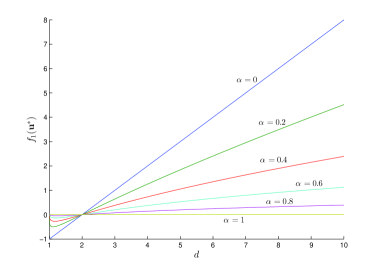
Figure 1: The behavior of the function $d-2+d^{1-\alpha}-d^{1-\alpha}(d-1)^{\alpha}$ for different values of the parameter $\alpha$.

Second, the function $h:\mathbb{R}^{d}\rightarrow\mathbb{R}$ is continuous and the Hessian of the surface $p(u_{1},\ldots,u_{d-1})=\phi(u_{1},u_{2},\ldots,u_{d-1},1-u_{1}-u_{2}-\cdots-u_{d-1})$ is

$$\frac{\partial^{2}p}{\partial u_{i}\partial u_{j}}=\alpha(\alpha-1)\times\begin{cases}(1-\sum_{k<d}u_{k})^{\alpha-2}-(\sum_{k<d}u_{k})^{\alpha-2}&i\not=j\\ u_{i}^{\alpha-2}-(1-u_{i})^{\alpha-2}+(1-\sum_{k<d}u_{k})^{\alpha-2}-(\sum_{k<d}u_{k})^{\alpha-2}&i=j\end{cases}\;,$$

which when evaluated at $\mathbf{u}^{*}$ yields the nondegenerate Hessian matrix

$$\alpha(\alpha-1)\left(d^{2-\alpha}-(1-1/d)^{\alpha-2}\right)\times\begin{pmatrix}2&1&1&\cdots&1\\ 1&2&1&\cdots&1\\ 1&1&2&\cdots&1\\ \vdots&\vdots&\ddots&\ddots&\vdots\\ 1&1&1&\cdots&2\end{pmatrix}\;.$$

As a result of all these conditions we have the Laplace-type asymptotic expansion [20, Page 500] at a boundary point, which is not a critical point:

$$\idotsint_{\mathscr{D}}h(\mathbf{u})\;\text{e}^{-\gamma^{\alpha}\phi(\mathbf{u})}\text{d}\mathbf{u}=\mathcal{O}(\gamma^{-\alpha(d+1)/2}\times\text{e}^{-\gamma^{\alpha}\phi(\mathbf{u}^{*})})\;,$$

where the constant $\phi(\mathbf{u}^{*})>0$. It follows that

$$\frac{\mathbb{E}\mathbb{I}\{M_{d}<\gamma\}\,Z^{2}}{\ell^{2}}\leqslant c_{2}\alpha^{d}\gamma^{d\alpha}\idotsint_{\mathscr{D}}h(\mathbf{u})\;\text{e}^{-\gamma^{\alpha}\phi(\mathbf{u})}\text{d}\mathbf{u}$$

$$=\mathcal{O}\big{(}\gamma^{\alpha(d-1)/2}\times\text{e}^{-\gamma^{\alpha}\phi(\mathbf{u}^{*})}\big{)}=\mathcal{O}\big{(}\text{e}^{\alpha(d-1)/2\ln\gamma-\gamma^{\alpha}\phi(\mathbf{u}^{*})}\big{)}\to 0\quad(\gamma\to\infty).$$

Hence the second term in (16) vanishes as $\gamma\to\infty$. $\Box$

4.1.2 Sum of Pareto random variables.

As in Example 3.3, we assume that $X_{i}$’s are independent and Pareto distributed random variables on $[1,\infty)$ with common parameter $\alpha>0$. The main result is the logarithmic efficiency of the second term of (16).

Proposition 4.6

For all $\varepsilon>0$

$$\limsup_{\gamma\to\infty}\frac{\mathbb{E}[Z^{2};M_{d}\leq\gamma]}{\ell^{2-\varepsilon}}=0.$$

Proof 4.7

The proof will be the result of a number of lemmas. First, similarly as in Lemma 4.4 we utilize expression (12) for rewriting the second moment as a product, and then we apply (14) and (15) to bound the factors. The result is that it is enough to prove that

$$\limsup_{\gamma\to\infty}\frac{1}{\ell^{2-\varepsilon}}\;\mathbb{E}_{f}\mathbb{I}\{M_{d}\leq\gamma,S_{d}>\gamma\}\prod_{i=1}^{d}\frac{\overline{F}(\gamma)}{\overline{F}(\gamma-X_{i})}=0.$$ (19)

Our approach is to consider a larger set containing $\{M_{d}\leq\gamma,S_{d}>\gamma\}$. For that purpose we define the we define the quantities

$$H_{n}(\gamma):=\mathbb{E}_{f}\bigg{[}\prod_{k=1}^{n}\frac{\overline{F}(\gamma)}{\overline{F}(\gamma-X_{k})};B_{n}\bigg{]},\qquad n\geq 2.$$

where

$$B_{n}=\{S_{n-1}\leq\gamma,S_{n}>\gamma,M_{n}\leq\gamma\},\qquad n=2,3,\ldots.$$

Observe that $\{M_{d}\leq\gamma,S_{d}>\gamma\}\subset\bigcup_{n=2}^{d}B_{n}$. Further to this, observing that $\overline{F}(\gamma)/\overline{F}(\gamma-x)\leq 1$ for all $x\geq 1$, we can set

$$\prod_{k=1}^{d}\frac{\overline{F}(\gamma)}{\overline{F}(\gamma-x_{k})}\leq\prod_{k=1}^{n}\frac{\overline{F}(\gamma)}{\overline{F}(\gamma-x_{k})},\qquad n\leq d.$$

In this way we arrive at the following inequality

$$\begin{split}\mathbb{E}_{f}\mathbb{I}\{&M_{d}\leq\gamma,S_{d}>\gamma\}\prod_{i=1}^{d}\frac{\overline{F}(\gamma)}{\overline{F}(\gamma-X_{i})}\\ &\leq\sum_{n=2}^{d}\mathbb{E}_{f}\bigg{[}\prod_{i=1}^{d}\frac{\overline{F}(\gamma)}{\overline{F}(\gamma-X_{i})};B_{n}\bigg{]}\\ &\leq\sum_{n=2}^{d}\mathbb{E}_{f}\bigg{[}\prod_{i=1}^{n}\frac{\overline{F}(\gamma)}{\overline{F}(\gamma-X_{i})};B_{n}\bigg{]}=\sum_{n=2}^{d}H_{n}(\gamma).\end{split}$$ (20)

Now, the quantities $H_{n}$ in the sum above can be written in integral form as

$$H_{n}(\gamma) =\int_{B_{n}}\bigg{(}\prod_{k=1}^{n}\frac{\overline{F}(\gamma)}{\overline{F}(\gamma-x_{k})}\bigg{)}\,\bigg{(}\prod_{k=1}^{n}f(x_{k})\bigg{)}\ {\mathrm{d}}x_{n}\,{\mathrm{d}}x_{n-1}\dots\,{\mathrm{d}}x_{2}\,{\mathrm{d}}x_{1}$$

$$=\int\limits_{1}^{\gamma-(n-2)}\ \ \int\limits_{1}^{\gamma-x_{1}-(n-3)}\!\dots\!\int\limits_{1}^{\gamma-x_{1}-\dots-x_{n-2}}\!\!\!\!\!\int\limits_{(\gamma-x_{1}-\dots-x_{n-1})\vee 1}^{\gamma}\prod_{k=1}^{n}\bigg{(}\frac{\gamma-x_{k}}{\gamma}\bigg{)}^{\alpha}\frac{\alpha}{x_{k}^{\alpha+1}}\ {\mathrm{d}}x_{n}\,{\mathrm{d}}x_{n-1}\dots\,{\mathrm{d}}x_{2}\,{\mathrm{d}}x_{1}.$$

Further, the change of variable $y_{k}=x_{k}/\gamma$ yields

$$\frac{\alpha^{n}}{\gamma^{n\alpha}}\!\int\limits_{\gamma^{-1}}^{1-(n-2)\gamma^{-1}}\ \ \int\limits_{\gamma^{-1}}^{1-y_{1}-(n-3)\gamma^{-1}}\!\dots\!\int\limits_{\gamma^{-1}}^{1-y_{1}-\dots-y_{n-2}}\!\!\!\!\!\!\int\limits_{(1-y_{1}-\dots-y_{n-1})\vee\gamma^{-1}}^{1}\prod_{k=1}^{n}\ L(y_{k})\ {\mathrm{d}}y_{n}\,{\mathrm{d}}y_{n-1}\dots\mathrm{d}y_{2}\,{\mathrm{d}}y_{1},$$

where

$$L(y):=(1-y)^{\alpha}\;y^{-(\alpha+1)},\qquad y\in(0,1].$$ (21)

In particular, it will be useful to write

$$H_{n}(\gamma)=\alpha^{n}\,\gamma^{-n\alpha}\,I_{n}(\gamma,1),$$ (22)

where the function $I_{n}(\gamma,1)$ is the multiple integral in the expression above. Moreover, $I_{n}(\gamma,\zeta)$ can be defined recursively for via

$$I_{n}(\gamma,\zeta):=\begin{cases}\int_{\zeta\vee\gamma^{-1}}^{1}L(y){\mathrm{d}}y,&\quad n=1,\\ \int_{\gamma^{-1}}^{\zeta-(n-2)\gamma^{-1}}L(y)\,I_{n-1}(\gamma,\zeta-y)\,{\mathrm{d}}y,&\quad n\geq 2.\end{cases}$$ (23)

Next we will prove that for $n=2,3,\ldots$, it holds that

$$\limsup_{\gamma\rightarrow\infty}\frac{I_{n}(\gamma,1)}{\gamma^{\alpha(n-2)}\ln\gamma}=0.$$ (24)

Since both numerator and denominator of (24) have limit $+\infty$, we can apply L’Hopital. Lemma 6.2 in the appendix provides a recursive expression for the derivative of the functions $I_{n}(\gamma,\zeta)$:

$$\frac{\partial}{\partial\gamma}I_{n}(\gamma,\zeta)=nL\big{(}\gamma^{-1}\big{)}\,I_{n-1}\big{(}\gamma,\zeta-\gamma^{-1}\big{)}\,\gamma^{-2},\qquad n=2,3,\ldots.$$ (25)

Therefore, we obtain

$$\limsup_{\gamma\to\infty}\frac{I_{n}(\gamma,1)}{\gamma^{\alpha(n-2)}\ln\gamma}=\limsup_{\gamma\to\infty}\frac{\frac{{\mathrm{d}}}{{\mathrm{d}}\gamma}I_{n}(\gamma,1)}{\frac{{\mathrm{d}}}{{\mathrm{d}}\gamma}\gamma^{\alpha(n-2)}\ln\gamma}$$

$$\quad=\limsup_{\gamma\to\infty}\frac{n\,L\big{(}\gamma^{-1}\big{)}\,I_{n-1}\big{(}\gamma,1-\gamma^{-1}\big{)}\,\gamma^{-2}}{\big{(}1+\alpha(n-2)\ln\gamma\big{)}\,\gamma^{\alpha(n-2)-1}},\qquad n=2,3,\ldots.$$ (26)

• $n=2$. The expression in (26) becomes

  $$\frac{2\,L\big{(}\gamma^{-1}\big{)}\,I_{1}\big{(}\gamma,1-\gamma^{-1}\big{)}\,\gamma^{-2}}{\gamma^{-1}}=\frac{2\,L\big{(}\gamma^{-1}\big{)}\,I_{1}\big{(}\gamma,1-\gamma^{-1}\big{)}}{\gamma}.$$

  Observe that

  $$L\big{(}\gamma^{-1}\big{)} =\big{(}1-\gamma^{-1}\big{)}^{\alpha}\,\gamma^{\alpha+1}=\mathcal{O}\big{(}\gamma^{\alpha+1}\big{)},\qquad\gamma\to\infty;$$

  $$L\big{(}1-\gamma^{-1}\big{)} =\gamma^{-\alpha}\,\big{(}1-\gamma^{-1}\big{)}^{-(\alpha+1)}=\mathcal{O}\big{(}\gamma^{-\alpha}\big{)},\qquad\gamma\to\infty;$$

  $$I_{1}\big{(}\gamma,1-\gamma^{-1}\big{)} =\int_{1-\gamma^{-1}}^{1}L(y)\,{\mathrm{d}}y\leqslant\gamma^{-1}L\big{(}1-\gamma^{-1}\big{)}=\mathcal{O}\big{(}\gamma^{-(\alpha+1)}\big{)},\qquad\gamma\to\infty,$$

  where the inequality follows because the function $L(y)$ is decreasing on $(0,1]$. Hence,

  $$\limsup_{\gamma\to\infty}\frac{2\,L\big{(}\gamma^{-1}\big{)}\,I_{1}\big{(}\gamma,1-\gamma^{-1}\big{)}}{\gamma}=\limsup_{\gamma\to\infty}\frac{(\mbox{a constant})\,\times\,\gamma^{\alpha+1}\,\gamma^{-(\alpha+1)}}{\gamma}=0.$$

• $n\geq 2$. Assume (24) holds for $n$. Then reasoning as above and using Lemma 6.4 for equality (i), we get for $n+1$

  $$\limsup_{\gamma\rightarrow\infty}\frac{I_{n+1}(\gamma,1)}{\gamma^{\alpha(n-1)}\ln\gamma}$$

  $$\quad=\limsup_{\gamma\to\infty}\frac{\frac{{\mathrm{d}}}{{\mathrm{d}}\gamma}I_{n+1}(\gamma,1)}{\frac{{\mathrm{d}}}{{\mathrm{d}}\gamma}\gamma^{\alpha(n-1)}\ln\gamma}$$

  $$\quad=\limsup_{\gamma\to\infty}\frac{(n+1)L\big{(}\gamma^{-1}\big{)}\,I_{n}\big{(}\gamma,1-\gamma^{-1}\big{)}\,\gamma^{-2}}{\big{(}1+\alpha(n-1)\ln\gamma\big{)}\,\gamma^{\alpha(n-1)-1}}$$

  $$\quad\overset{\rm(i)}{=}\limsup_{\gamma\to\infty}\frac{(n+1)L\big{(}\gamma^{-1}\big{)}\,\Big{(}I_{n}\big{(}\gamma,1\big{)}+o(1)\Big{)}\,\gamma^{-2}}{\big{(}1+\alpha(n-1)\ln\gamma\big{)}\,\gamma^{\alpha(n-1)-1}}$$

  $$\quad=\limsup_{\gamma\to\infty}\frac{(\mbox{a constant})\,\times\,\gamma^{\alpha+1}\,I_{n}\big{(}\gamma,1\big{)}\,\gamma^{-2}+o(1)}{(\mbox{a constant})\,\times\,\gamma^{\alpha(n-1)-1}\,\ln\gamma}$$

  $$\quad=\limsup_{\gamma\to\infty}\ \ (\mbox{a constant})\,\times\,\frac{I_{n}\big{(}\gamma,1\big{)}+o(1)}{\gamma^{\alpha(n-2)}\,\ln\gamma}=0$$

Putting together these arguments we can complete the proof of the Proposition:

$$\limsup_{\gamma\to\infty}\frac{\mathbb{E}\mathbb{I}\{M_{d}\leq\gamma\}\,Z^{2}}{\ell^{2-\varepsilon}}$$

$$\quad\overset{\eqref{e:enough}}{\leq}\limsup_{\gamma\to\infty}\frac{1}{\ell^{2-\varepsilon}}\;\mathbb{E}_{f}\mathbb{I}\{M_{d}\leq\gamma,S_{d}>\gamma\}\prod_{i=1}^{d}\frac{\overline{F}(\gamma)}{\overline{F}(\gamma-X_{i})}$$

$$\quad\overset{\eqref{e:sumhn}}{\leq}\limsup_{\gamma\to\infty}\frac{\sum_{n=2}^{d}H_{n}(\gamma)}{\ell^{2-\varepsilon}}$$

$$\quad\overset{\eqref{e:defIn}}{=}\limsup_{\gamma\to\infty}\sum_{n=2}^{d}\frac{\alpha^{n}I_{n}(\gamma)}{\gamma^{\alpha n}\,\ell^{2-\varepsilon}}$$

Now notice that

$$\ell=\overline{F^{*d}}(\gamma)\geq\overline{F}(\gamma)=\gamma^{-\alpha},$$

thus, for $\varepsilon<1/\alpha$ (that is, $\varepsilon\alpha<1$)

$$\ell^{2-\varepsilon}\geq\gamma^{-2\alpha}\,\gamma^{\alpha\varepsilon}\geq\gamma^{-2\alpha}\,\ln\gamma,\qquad\gamma\to\infty.$$

Combining this with above, we get

$$\limsup_{\gamma\to\infty}\sum_{n=2}^{d}\frac{\alpha^{n}I_{n}(\gamma)}{\gamma^{\alpha n}\,\ell^{2-\varepsilon}}\leq\sum_{n=2}^{d}\alpha^{n}\limsup_{\gamma\to\infty}\frac{I_{n}(\gamma)}{\gamma^{\alpha(n-2)}\,\ln\gamma}=0$$

4.2 Light-tailed case

In this section we consider the case where $F$ belongs to a subfamily of light-tailed distributions as defined by Embrechts and Goldie [10]. We say that a distribution $F$ belongs to the Embrechts-Goldie family of distributions indexed by the parameter $\theta\geq 0$ and denoted $\mathcal{L}(\theta)$, if

$$\lim_{\gamma\rightarrow\infty}\frac{\overline{F}(\gamma+x)}{\overline{F}(\gamma)}=\text{e}^{-\theta x}.$$ (27)

If $\theta$ is strictly larger than $0$ then $\mathcal{L}(\theta)$ contains light-tailed distributions exclusively and is often referred as the exponential class. This is a very rich class of distributions that includes several well know light-tailed distributions such as the exponential, gamma and phase-type. In contrast, if $\theta=0$, then $\mathcal{L}(0)$ corresponds to the class of long-tailed distributions which is a large subclass of heavy-tailed distributions. In this section we concentrate on the light-tailed case $\theta>0$, but in order to derive our efficiency statements we draw some results for the class of the so called long-tailed functions (cf. [11, Definition 2.14]). More precisely, $h$ is long-tailed if it is ultimately positive and

$$\lim_{\gamma\rightarrow\infty}\frac{h(\gamma+x)}{h(\gamma)}=1,\qquad\forall x.$$ (28)

Obviously, if $F\in\mathcal{L}(0)$, then the tail probability $\overline{F}$ is long tailed. Important properties for the exponential class ($\theta>0$) are

• $\mathcal{L}(\theta)$ is closed under convolutions [10, Theorem 3]. That is, if $F\in\mathcal{L}(\theta)$, then the $d$-fold convolution $F^{*d}\in\mathcal{L}(\theta)$.

• Define for $\alpha>0$ the distribution $G(x)=1-\big{(}\overline{F}(x)\big{)}^{\alpha}$. One can easily check that $G\in\mathcal{L}(\alpha\theta)$ whenever $F\in\mathcal{L}(\theta)$.

• The tail probability can be decomposed into the product of an exponential and a long tailed function

  $$\overline{F}(\gamma)=\text{e}^{-\theta\gamma}h(\gamma).$$ (29)

Decomposition (29) will be useful for proving efficiency of the proposed estimator, but it is also interesting on its own. To verify it we define $h(\gamma):=\overline{F}(\gamma)\;\text{e}^{\theta\gamma}$. Since $F\in\mathcal{L}(\theta)$ it follows that

$$\lim_{\gamma\rightarrow\infty}\frac{h(\gamma+x)}{h(\gamma)}=\lim_{\gamma\rightarrow\infty}\frac{h(\gamma+x)\,\text{e}^{-\theta(\gamma+x)}}{h(\gamma)\,\text{e}^{-\theta(\gamma+x)}}=\lim_{\gamma\rightarrow\infty}\frac{\overline{F}(\gamma+x)}{\overline{F}(\gamma)\,\text{e}^{-\theta x}}=1.$$

The next property states that the asymptotic decay of a long-tailed function is slower than the exponential rate [11, Lemma 2.17]. More precisely, if $h$ is long tailed, then

$$\lim_{\gamma\rightarrow\infty}\frac{h(\gamma)}{\text{e}^{-\varepsilon\gamma}}=\infty,\qquad\forall\varepsilon>0.$$ (30)

These properties will be employed to construct an asymptotic upper bound for the semi-parametric estimator. In particular, the following Lemma shows that the ratio of two tail convolutions of the same distribution in $\mathcal{L}(\theta)$ cannot increase/decrease faster than at exponential rate.

Lemma 4.8

Let $F\in\mathcal{L}(\theta)$, $\theta>0$, and $d_{1},d_{2}\in{\rm Nature}$. Then ${\overline{F^{*d_{1}}}(\gamma)}\Big{/}\,{\overline{F^{*d_{2}}}(\gamma)}=o(\text{e}^{\varepsilon\gamma}),\qquad\forall\varepsilon>0$.

Proof 4.9

Since $\mathcal{L}(\theta)$ is closed by convolution, then $F^{*d_{1}},F^{*d_{2}}\in\mathcal{L}(\theta)$ and their tail distributions have decompositions as in (29) for some long tailed functions $h_{1}$ and $h_{2}$. Therefore

$$\frac{\overline{F^{*d_{1}}}(\gamma)}{\overline{F^{*d_{2}}}(\gamma)}=\frac{h_{1}(\gamma)\text{e}^{-\theta\gamma}}{h_{2}(\gamma)\text{e}^{-\theta\gamma}}=\frac{h_{1}(\gamma)}{h_{2}(\gamma)}.$$

We first argue that both $h_{1}(\cdot)/h_{2}(\cdot)$ and its reciprocal function are long-tailed. This is so, because they are ultimately positive, and

$$\frac{h_{1}(\gamma+x)/h_{2}(\gamma+x)}{h_{1}(\gamma)/h_{2}(\gamma)}=\frac{h_{1}(\gamma+x)}{h_{1}(\gamma)}\,\times\,\frac{h_{2}(\gamma)}{h_{2}(\gamma+x)}\to 1.$$

The reciprocal function goes similarly. Thus, $h_{2}(\cdot)/h_{1}(\cdot)$ satisfies condition (30), which says

$$\lim_{\gamma\rightarrow\infty}\frac{h_{2}(\gamma)/h_{1}(\gamma)}{\text{e}^{-\varepsilon\gamma}}=\infty.$$

Clearly, this is equivalent to

$$\lim_{\gamma\rightarrow\infty}\frac{h_{1}(\gamma)/h_{2}(\gamma)}{\text{e}^{\varepsilon\gamma}}=0.$$

$\Box$

We also have the following.

Assumption A: Let $h$ be a long-tailed function such that $h(x)>0$ for all $x\geq 0$. Then $G(\gamma):=\sup\{h(\gamma)/h(x):0\leq x\leq\gamma\}=o(\text{e}^{\varepsilon\gamma})$ for all $\varepsilon>0$.

Proposition 4.10 (Logarithmic efficiency of $\widehat{\ell}$)

If Assumption A holds, the estimator $Z=\mathbb{I}\{S(\mathbf{X})>\gamma\}\frac{f(\mathbf{X})}{g(\mathbf{X})}$ satisfies

$$\lim_{\gamma\uparrow\infty}\frac{\mathbb{E}Z^{2}}{\ell^{2-\varepsilon}(\gamma)}=0,\qquad\forall\varepsilon>0\;.$$

Proof 4.11

Recall

$$\mathbb{E}Z^{2}=\mathbb{E}_{f}\mathbb{I}\{S(\mathbf{X})>\gamma\}\,\prod_{i=1}^{d}\frac{\overline{F^{*d}}(\gamma)}{\overline{F^{*(d-1)}}(\gamma-X_{i})}.$$

We write

$$\prod_{i=1}^{d}\frac{\overline{F^{*d}}(\gamma)}{\overline{F^{*(d-1)}}(\gamma-X_{i})}=H(\gamma)\prod_{i=1}^{d}\frac{\overline{F^{*(d-1)}}(\gamma)}{\overline{F^{*(d-1)}}(\gamma-X_{i})},$$

where $H(\gamma):=\Big{[}\overline{F^{*d}}(\gamma)\big{/}\overline{F^{*(d-1)}}(\gamma)\Big{]}^{d}$. Since $F^{*(d-1)}\in\mathcal{L}(\theta)$ we can use the decomposition (29) to write $\overline{F^{*(d-1)}}(\gamma)=h(\gamma)\text{e}^{-\theta\gamma}$ for some $h(\cdot)$ long tailed function. Hence, we obtain the following bound

$$\prod_{i=1}^{d}\frac{\overline{F^{*(d-1)}}(\gamma)}{\overline{F^{*(d-1)}}(\gamma-X_{i})}=\prod_{i=1}^{d}\frac{h(\gamma)}{h(\gamma-X_{i})}\;\frac{\text{e}^{-\theta\gamma}}{\text{e}^{-\theta(\gamma-X_{i})}}\leq\bigg{(}\sup_{0\leq x\leq\gamma}\frac{h(\gamma)}{h(\gamma-x)}\bigg{)}^{d}\prod_{i=1}^{d}{\text{e}^{-\theta X_{i}}}=\big{(}G(\gamma)\big{)}^{d}\,\text{e}^{-\theta S(\mathbf{X})}$$

where $G(\gamma):=\sup_{0\leq x\leq\gamma}\big{\{}{h(\gamma)}\big{/}{h(\gamma-x)}\big{\}}$. Using these we obtain

$$\frac{{\mathbb{E}}\,Z^{2}}{\ell^{2-\varepsilon}(\gamma)}\leq\frac{H(\gamma)G^{d}(\gamma)}{\ell^{2-\varepsilon}(\gamma)}\mathbb{E}_{f}\mathbb{I}\{S(\mathbf{X})>\gamma\}\,\text{e}^{-\theta S(\mathbf{X})},$$

where $\theta>0$. Hence,

$$\mathbb{E}_{f}\mathbb{I}\{S(\mathbf{X})>\gamma\}\,\text{e}^{-\theta S(\mathbf{X})}\leqslant\text{e}^{-\theta\gamma}\mathbb{P}_{f}(S(\mathbf{X})>\gamma)=\text{e}^{-\theta\gamma}\,\ell.$$

Thus we get

$$\frac{{\mathbb{E}}\,Z^{2}}{\ell^{2-\varepsilon}(\gamma)}\leqslant\frac{H(\gamma)G^{d}(\gamma)\text{e}^{-\theta\gamma}}{\ell^{1-\varepsilon}(\gamma)}.$$

Applying the properties of the exponential class we can write

$$\ell^{1-\varepsilon}=\big{(}\overline{F^{*d}}(\gamma)\big{)}^{1-\varepsilon}=\text{e}^{-\theta(1-\varepsilon)\gamma}h_{d}(\gamma)$$

for some long tailed function $h_{d}$. In consequence,

$$\limsup_{\gamma\rightarrow\infty} \frac{{\mathbb{E}}\,Z^{2}}{\ell^{2-\varepsilon}(\gamma)}\leqslant\limsup_{\gamma\rightarrow\infty}\frac{H(\gamma)G^{d}(\gamma)\text{e}^{-\theta\gamma}}{\ell^{1-\varepsilon}(\gamma)}$$

$$=\limsup_{\gamma\rightarrow\infty}\frac{H(\gamma)G^{d}(\gamma)\text{e}^{-\theta\gamma}}{h_{d}(\gamma)\text{e}^{-(1-\varepsilon)\theta\gamma}}=\limsup_{\gamma\rightarrow\infty}\frac{H(\gamma)G^{d}(\gamma)}{h_{d}(\gamma)}\text{e}^{-\varepsilon\theta\gamma}.$$

Now, property (29) and Lemma 4.8 and Lemma 4.9 imply that none of the functions $H$, $G$, $h_{d}^{-1}$ and their product cannot increase at exponential rate, namely $H(\gamma)G^{d}(\gamma)/h_{d}(\gamma)=o(\text{e}^{\theta\varepsilon\gamma})$. Hence, the last limit is 0. $\Box$

5 Conclusions

In this paper we have described a procedure for implementing an optimal cross-entropy importance sampling density for the purpose of estimating a rare-event probability, indexed by the rarity parameter $\gamma$. The goal is to estimate the optimal importance sampling density for a finite $\gamma$ within the class of all densities in product form. This optimal importance sampling density is typically not available analytically and this is why in practical simulations we estimate it via MCMC simulation from the minimum variance pdf. The numerical examples suggest that the resulting estimator can yield significantly better efficiency compared to many currently recommended estimators. The same procedure is efficient in both light- and heavy-tailed cases. This is especially relevant for probabilities involving the Weibull distribution with tail index $\alpha<1$, but close to unity. This setting yields behavior intermediate between the typical heavy- and light-tailed behavior expected of rare-events. As a result, while existing procedures are inefficient or fail completely, our method estimates reliably Weibull probabilities for any values of $\alpha$, including $\alpha>1$.

The practical implementation of the proposed method depends on a preliminary MCMC step, which is a powerful, but poorly understood heuristic that needs further investigation. In this article we have established the efficiency of the method in the light- and heavy-tailed case, but have done so by ignoring any errors arising from the preliminary MCMC step. Future work will need to address the impact of the MCMC approximation on the quality of the estimator. A good starting point for such an analysis might be to consider the probabilistic relative error efficiency concept introduced in [19].

6 Appendix

6.1 Proofs. Section 2.2

Proof 6.1 (Proof of Lemma 2.2)

First note that for any single-variate function $h$:

$$\int_{\mathbb{R}^{d}} h(x_{1})\pi(\mathbf{x})\,\text{d}\mathbf{x}=\int_{\mathbb{R}}h(x_{1})\Big{(}\int_{\mathbb{R}^{d-1}}\pi(x_{1},x_{2},\ldots,x_{d})\,\text{d}x_{2}\cdots\text{d}x_{d}\Big{)}\,\text{d}x_{1}$$

$$=\int h(x_{1})\pi_{1}(x_{1})\,\text{d}x_{1}.$$

Next, using the properties of the cross-entropy distance we have that

$$\pi_{1}=\mathop{\rm argmin}_{g_{1}\in\mathscr{G}_{1}}\int\pi_{1}(x_{1})\ln\left(\frac{\pi_{1}(x_{1})}{g_{1}(x_{1})}\right)\text{d}x_{1}=\operatornamewithlimits{argmax}_{g_{1}\in\mathscr{G}_{1}}\int\pi_{1}(x_{1})\ln g_{1}(x_{1})\,\text{d}x_{1}.$$

Applying these two observations for any $i=1,\ldots,d$ gives

$$\operatornamewithlimits{argmax}_{g_{1},\ldots,g_{d}\in\mathscr{G}_{1}} \int\pi(\mathbf{x})\ln\left(\prod_{i=1}^{d}g_{i}(x_{i})\right)\text{d}\mathbf{x}$$

$$=\operatornamewithlimits{argmax}_{g_{1},\ldots,g_{d}\in\mathscr{G}_{1}}\sum_{i=1}^{d}\int\pi(\mathbf{x})\ln g_{i}(x_{i})\,\text{d}\mathbf{x}$$

$$=\operatornamewithlimits{argmax}_{g_{1},\ldots,g_{d}\in\mathscr{G}_{1}}\sum_{i=1}^{d}\int\pi_{i}(x_{i})\ln g_{i}(x_{i})\,\text{d}x_{i}=\sum_{i=1}^{d}\operatornamewithlimits{argmax}_{g_{i}\in\mathscr{G}_{1}}\int\pi_{i}(x_{i})\ln g_{i}(x_{i})\,\text{d}x_{i},$$

from where we obtain the solution $g_{i}=\pi_{i}$ for all $i=1,\ldots,d$. $\Box$

6.2 Proofs. Section 4.1

Lemma 6.2

Assume $\zeta\geq n\gamma^{-1}$. Then

$$\frac{\partial}{\partial\gamma}I_{n}(\gamma,\zeta)=n\,L\big{(}\gamma^{-1}\big{)}\,I_{n-1}\big{(}\gamma,\zeta-\gamma^{-1}\big{)}\,\gamma^{-2},\qquad n=2,3,\ldots.$$ (31)

Proof 6.3

The proof is by induction. Recall the recursive introduction of the $I_{n}$ functions:

$$I_{1}(\gamma,\zeta) =\int_{\zeta\,\vee\,\gamma^{-1}}^{1}L(y)\,{\mathrm{d}}y;$$

$$I_{n}(\gamma,\zeta) =\int_{\gamma^{-1}}^{\zeta-(n-2)\gamma^{-1}}L(y)\,I_{n-1}(\gamma,\zeta-y)\,{\mathrm{d}}y,\qquad n=2,3,\ldots$$

First consider

$$\frac{\partial}{\partial\gamma}I_{2}(\gamma,\zeta)=\frac{\partial}{\partial\gamma}\int_{\gamma^{-1}}^{\zeta-\gamma^{-1}}L(y)\,I_{1}(\gamma,\zeta-y)\,{\mathrm{d}}y+\frac{\partial}{\partial\gamma}\,\int_{\zeta-\gamma^{-1}}^{\zeta}L(y)\,{\mathrm{d}}y\,I_{1}(\gamma,\gamma^{-1})$$

$$\quad=\bigg{[}L(\zeta-\gamma^{-1})I_{1}(\gamma,\gamma^{-1})-L\big{(}\gamma^{-1}\big{)}\,I_{1}\big{(}\gamma,\zeta-\gamma^{-1}\big{)}-L(\zeta-\gamma^{-1})I_{1}(\gamma,\gamma^{-1})-I_{1}(\gamma,\zeta-\gamma^{-1})L(\gamma^{-1})\bigg{]}\,\frac{{\mathrm{d}}}{{\mathrm{d}}\gamma}\gamma^{-1}$$

$$\quad=2\,L\big{(}\gamma^{-1}\big{)}\,I_{1}\big{(}\gamma,\zeta-\gamma^{-1}\big{)}\,\gamma^{-2}.$$

Next, assume that (31) holds for $n$. Then

$$\frac{\partial}{\partial\gamma}I_{n+1}(\gamma,\zeta)=\frac{\partial}{\partial\gamma}\int_{\gamma^{-1}}^{\zeta-(n-1)\gamma^{-1}}L(y)\,I_{n}(\gamma,\zeta-y)\,{\mathrm{d}}y$$

$$\quad=L(\zeta-(n-1)\gamma^{-1})\,I_{n}\big{(}\gamma,(n-1)\gamma^{-1}\big{)}\,\frac{{\mathrm{d}}}{{\mathrm{d}}\gamma}\big{(}\zeta-(n-1)\gamma^{-1}\big{)}-L(\gamma^{-1})\,I_{n}\big{(}\gamma,\zeta-\gamma^{-1}\big{)}\,\frac{{\mathrm{d}}}{{\mathrm{d}}\gamma}\gamma^{-1}$$

$$\qquad+\int_{\gamma^{-1}}^{\zeta-(n-1)\gamma^{-1}}L(y)\,\frac{\partial}{\partial\gamma}I_{n}(\gamma,\zeta-y)\,{\mathrm{d}}y$$

$$\quad=0+L(\gamma^{-1})\,I_{n}\big{(}\gamma,\zeta-\gamma^{-1}\big{)}\,\gamma^{-2}+\int_{\gamma^{-1}}^{\zeta-(n-1)\gamma^{-1}}L(y)\,n\,L\big{(}\gamma^{-1}\big{)}\,I_{n-1}\big{(}\gamma,\zeta-\gamma^{-1}-y\big{)}\,\gamma^{-2}\,{\mathrm{d}}y$$

$$\quad=L(\gamma^{-1})\,I_{n}\big{(}\gamma,\zeta-\gamma^{-1}\big{)}\,\gamma^{-2}+n\,L\big{(}\gamma^{-1}\big{)}\int_{\gamma^{-1}}^{\zeta-\gamma^{-1}-(n-2)\gamma^{-1}}L(y)\,I_{n-1}\big{(}\gamma,\zeta-\gamma^{-1}-y\big{)}\,{\mathrm{d}}y\,\gamma^{-2}$$

$$\quad=L(\gamma^{-1})\,I_{n}\big{(}\gamma,\zeta-\gamma^{-1}\big{)}\,\gamma^{-2}+n\,L\big{(}\gamma^{-1}\big{)}I_{n}\big{(}\gamma,\zeta-\gamma^{-1}\big{)}\,\gamma^{-2}$$

$$\quad=(n+1)L(\gamma^{-1})\,I_{n}\big{(}\gamma,\zeta-\gamma^{-1}\big{)}\,\gamma^{-2}$$

$\Box$

Lemma 6.4

For $n=1,2,\ldots$:

$$I_{n}\big{(}\gamma,\zeta-\gamma^{-1}\big{)}=I_{n}(\gamma,\zeta)+o(1),\qquad\gamma\to\infty.$$ (32)

Proof 6.5

Apply induction and the the recursive definition of $I_{n}$ functions.

• $n=1$.

  $$I_{1} \big{(}\gamma,\zeta-\gamma^{-1}\big{)}=\int_{\zeta-\gamma^{-1}}^{1}L(y)\,{\mathrm{d}}y$$

  $$=I_{1}(\gamma,\zeta)+\int_{\zeta-\gamma^{-1}}^{\zeta}L(y)\,{\mathrm{d}}y$$

  $$=I_{1}(\gamma,\zeta)+\gamma^{-1}L(\eta),$$

  for some $\eta\in(\zeta-\gamma^{-1},\zeta)$ (mean value theorem). Clearly, the second term is $o(1)$ for $\gamma\to\infty$.

• $n\geq 1$. Assume (32) holds. Then

  $$I_{n+1} \big{(}\gamma,\zeta-\gamma^{-1}\big{)}=\int_{\gamma^{-1}}^{\zeta-n\gamma^{-1}}L(y)I_{n}\big{(}\gamma,\zeta-\gamma^{-1}-y\big{)}\,{\mathrm{d}}y$$

  $$=\int_{\gamma^{-1}}^{\zeta-(n-1)\gamma^{-1}}L(y)\Big{(}I_{n}(\gamma,\zeta-y)+o(1)\Big{)}\,{\mathrm{d}}y-\int_{\zeta-n\gamma^{-1}}^{\zeta-(n-1)\gamma^{-1}}L(y)I_{n}\big{(}\gamma,\zeta-\gamma^{-1}-y\big{)}\,{\mathrm{d}}y$$

  $$=I_{n+1}(\gamma,\zeta)+o(1)\,\int_{\gamma^{-1}}^{\zeta-(n-1)\gamma^{-1}}L(y)\,{\mathrm{d}}y-\gamma^{-1}L(\eta)I_{n}\big{(}\gamma,\zeta-\gamma^{-1}-\eta\big{)}$$

  $$=I_{n+1}(\gamma,\zeta)+o(1),\qquad\gamma\to\infty.$$

$\Box$

References

- [1] S. Asmussen and P. W. Glynn. Stochastic Simulation: Algorithms and Analysis. Springer-Verlag, New York, 2007.
- [2] S. Asmussen and D. P. Kroese. Improved algorithms for rare event simulation with heavy tails. Advances in Applied Probability, 38(2), 2006.
- [3] S. Asmussen, D. P. Kroese, and R. Y. Rubinstein. Heavy tails, importance sampling and cross-entropy. Stochastic Models, 21(1), 2005.
- [4] Søren Asmussen and Dominik Kortschak. On error rates in rare event simulation with heavy tails. In Proceedings of the Winter Simulation Conference, page 38. Winter Simulation Conference, 2012.
- [5] Z. I. Botev and D. P. Kroese. Efficient Monte Carlo simulation via the generalized splitting method. Statistics and Computing, 2010. DOI:10.1007/s11222-010-9201-4.
- [6] Zdravko I. Botev, Pierre L’Ecuyer, and Bruno Tuffin. Markov chain importance sampling with applications to rare event probability estimation. Statistics and Computing, 23(2):271–285, 2013.
- [7] J. C. C. Chan and D. P. Kroese. Improved cross-entropy method for estimation. manuscript, 2011.
- [8] Joshua C.C. Chan, Peter W. Glynn, and Dirk P. Kroese. A comparison of cross-entropy and variance minimization strategies. Journal of Applied Probability, 48:183–194, 2011.
- [9] P. Embrechts, C. Kluppelberg, and T. Mikosch. Modelling extremal events. Springer-Verlag, Berlin, 1997.
- [10] Paul Embrechts and Charles Goldie. On closure and factorisation properties of subexponential and related distributions. Cambridge Univ Press, 1980.
- [11] Sergey Foss, Dmitry Korshunov, and Stan Zachary. An introduction to heavy-tailed and subexponential distributions. Springer, 2011.
- [12] Samim Ghamami and Sheldon Ross. Improving the Asmussen–Kroese-type simulation estimators. Journal of Applied Probability, 49(4):1188–1193, 2012.
- [13] Jürgen Hartinger and Dominik Kortschak. On the efficiency of the Asmussen–Kroese-estimator and its application to stop-loss transforms. Blätter der DGVFM, 30(2):363–377, 2009.
- [14] S. Juneja. Estimating tail probabilities of heavy tailed distributions with asymptotically zero relative error. Queueing Systems, 57(2-3):115–127, 2007.
- [15] D. P. Kroese, R. Y. Rubinstein, and P. W. Glynn. The cross-entropy method for estimation. In V. Govindaraju and C.R. Rao, editors, Handbook of Statistics, Volume 31: Machine Learning. North Holland, 2011.
- [16] D. P. Kroese, T. Taimre, and Z. I. Botev. Handbook of Monte Carlo methods. John Wiley & Sons, New York, 2011.
- [17] P. L’Ecuyer, J. Blanchet, B. Tuffin, and P. W. Glynn. Asymptotic robustness of estimators in rare-event simulation. ACM Transactions on Modeling and Computer Simulation, 20(1), 2010. Article 6.
- [18] R. Y. Rubinstein and D. P. Kroese. The Cross-Entropy Method: A Unified Approach to Combinatorial Optimization, Monte-Carlo Simulation and Machine Learning. Springer-Verlag, New York, 2004.
- [19] Bruno Tuffin and Ad Ridder. Probabilistic bounded relative error for rare event simulation learning techniques. In Proceedings of the Winter Simulation Conference, page 40. Winter Simulation Conference, 2012.
- [20] Roderick Wong. Asymptotic approximation of integrals, volume 34. Society for Industrial and Applied Mathematics, 2001.