Kepler-like Multi-Plexing for Mass Production of Microlens Parallaxes

Abstract

We show that a wide-field Kepler-like satellite in Solar orbit could obtain microlens parallaxes for several thousand events per year that are identified from the ground, yielding masses and distances for several dozen planetary events. This is roughly an order of magnitude larger than previously-considered narrow-angle designs. Such a satellite would, in addition, roughly double the number of planet detections (and mass/distance determinations). It would also yield a trove of brown-dwarf binaries with masses, and distances and (frequently) full orbits, enable new probes of the stellar mass function, and identify isolated black-hole candidates. We show that the actual Kepler satellite, even with degraded pointing, can demonstrate these capabilities and make substantial initial inroads into the science potential. We discuss several “Deltas” to the Kepler satellite aimed at optimizing microlens parallax capabilities. Most of these would reduce costs. The wide-angle approach advocated here has only recently become superior to the old narrow-angle approach, due to the much larger number of ground-based microlensing events now being discovered.

1 Introduction

Microlens parallaxes have become a crucial focus of microlensing experiments. For the overwhelming majority of microlensing events, one does not know the lens mass, distance, or velocity separately, but only the Einstein timescale $t_{\rm E}$, which is a combination of these

$$t_{\rm E}={\theta_{\rm E}\over\mu_{\rm geo}};\quad\theta_{\rm E}^{2}=\kappa M\pi_{\rm rel};\quad\kappa\equiv{4G\over c^{2}\,{\rm AU}}\simeq 8.1\,{{\rm mas}\over M_{\odot}}.$$ (1)

Here $M$ is the lens mass, $\theta_{\rm E}$ is the Einstein radius, $\pi_{\rm rel}$ is the lens-source relative parallax, and $\mu_{\rm geo}$ is the lens-source relative proper motion in the geocentric frame at the peak of the event.

Microlens parallaxes have become a focus because of the increasing number of microlens planet detections. If the planet can be detected well enough to be characterized, it is almost always because the source star passed over or very near a “caustic” structure induced by the planet. This enables one to measure the size of the source radius relative to the Einstein radius: $\rho=\theta_{*}/\theta_{\rm E}$. Since $\theta_{*}$ itself is routinely measurable from the position of the source on an instrumental color-magnitude diagram (Yoo et al., 2004), this means that $\theta_{\rm E}$ is measured in almost all planetary events.

Hence, if the microlens parallax

$$\pi_{\rm E}={\pi_{\rm rel}\over\theta_{\rm E}};\quad M={\theta_{\rm E}\over\kappa\pi_{\rm E}}$$ (2)

could be routinely measured, it would yield masses and distances for essentially all microlens planets. Such mass measurements would yield detailed features in the planet mass function that are currently washed out by the $M\sin i$ degeneracy for Doppler (RV) detected planets, and by severe selection for current transit surveys. Because microlensing planets are detected from the Galactic bulge almost to the solar neighborhood, the distance measurements would yield the Galactic distribution of planets, and would in particular test for relative planet frequency in the very different environments of the Galactic disk and bulge.

Unfortunately, microlens parallax measurements today are anything but “routine”. As specified in Equation (2), $\pi_{\rm E}$ quantifies the size of the trigonometric lens-source parallax oscillations (due to Earth orbit) compared to the Einstein radius. In principle the photometric effect of these oscillations should just scale with $\pi_{\rm E}$. However, because $t_{\rm E}\ll\rm yr$ for most microlensing events, the lens-source path is mainly just displaced from what would be seen from the Sun, rather than oscillating about it. Hence, $\pi_{\rm E}$ measurements are both rare and very heavily biased toward long events.

However, a quarter century before Gould (1992) proposed measuring $\pi_{\rm E}$ from such annual oscillations, Refsdal (1966) had already pointed to a way out: put a satellite in solar orbit to monitor the microlensing event simultaneously with Earth-bound observations. There are a number of complications introduced by this geometry (Refsdal, 1966; Gould, 1994, 1995), which we review below, but these have been systematically addressed in subsequent work and are now generally regarded as tractable.

The key obstacle to launching such a satellite was that the potential scientific return was too modest to justify its substantial cost. At the time that microlens parallax satellites were first proposed circa 1996, relatively few microlensing events were being discovered and almost none had $\theta_{\rm E}$ measurements. Hence, $\pi_{\rm E}$ measurements would not yield masses or distances but only somewhat lower statistical errors on Bayesian mass estimates. In addition, no planets were being discovered, so that any masses that were measured would be overwhelmingly of luminous stars, whose mass function is more easily probed by photometric surveys.

In the meantime, the rate of microlensing event detections has grown by almost 2 orders of magnitude and continues to grow. Yet the basic concept of a parallax satellite equipped with a narrow-angle camera that would cycle through a list of ongoing events has remained the same.

Here we argue that a wide-field camera in solar orbit, similar to Kepler, is a far better match to the requirements of microlensing parallaxes. Its multiplexing capabilities more than compensate for the inevitable increase in “sky” background due to the larger pixels and point spread function (PSF) that are required to continuously monitor tens of square degrees. In addition, by carrying out continuous monitoring from a position that is well separated in the Einstein ring, the satellite would essentially double the number of planets discovered. Finally, such a parallax satellite would be uniquely capable of many other investigations, such as studies of brown dwarf binaries.

2 Nature of Microlensing Parallax

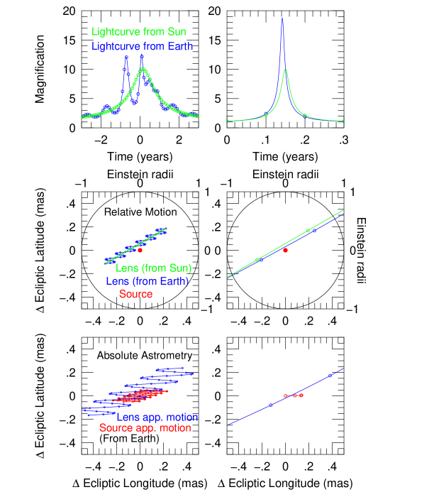
Figure 1: Parallax effect for illustrative (left) and realistic (right) microlensing events. Bottom: absolute trigonometric parallax and proper motion (ppm). Middle: relative trigonometric (lower/left labels) and microlensing (upper/right labels) ppm. Top: resulting lightcurves from Earth (blue) and Sun (green).

Figure 1 illustrates the relation of microlensing to trigonometric parallax. The bottom panels show the absolute astrometry due to trigonometric parallax and proper motion (ppm) of the source and lens separately. The middle panels show relative ppm (both trigonometric and microlensing, but with different scaling). The top panels show the resulting lightcurves as seen from both the Sun and Earth. Both columns have $\pi_{\rm rel}=60\,{\mu\rm as}$ and $M=0.5\,M_{\odot}$ (typical values for events with disk lenses and bulge sources), corresponding to $\theta_{\rm E}=0.5\,{\rm mas}$ and $\pi_{\rm E}=0.12$. The right column has a heliocentric proper motion $\mu_{\rm hel}=5\,{\rm mas}\,{\rm yr}^{-1}$ (also typical), while the left column has a highly atypical $\mu_{\rm hel}=0.1\,{\rm mas}\,{\rm yr}^{-1}$, which only occurs in about $10^{-5}$ of all events.

The left column illustrates the basic principle, but the right column illustrates the basic problem: in typical events the lens does not oscillate about its position as seen from the Sun, but is primarily displaced from it (easily seen in plot but unobservable from Earth). The observable effect is then a slight distortion (imperceptible here) to the light curve, rather than oscillations. The figure makes clear why microlensing parallax is a vector

$${\mbox{\boldmath$\pi$}}_{{\rm E},{\rm geo}}=\pi_{\rm E}{{\mbox{\boldmath$\mu$}}_{\rm geo}\over\mu_{\rm geo}};\quad{\mbox{\boldmath$\pi$}}_{{\rm E},{\rm hel}}=\pi_{\rm E}{{\mbox{\boldmath$\mu$}}_{\rm hel}\over\mu_{\rm hel}},$$ (3)

for which the proper motion provides the direction, whereas trigonometric parallax is a scalar. That is, in microlensing the direction is known only if the parallax is measured. It also makes clear why the “microlensing proper motion” ($\mu_{\rm E}\equiv t_{\rm E}^{-1}$) is a scalar and is measured in the geocentric frame: $\mu_{\rm E}=\mu_{\rm geo}/\theta_{\rm E}$. That is, in the absence of parallax information (the usual case), there is only information about the geocentric rate of passage through the Einstein ring.

Finally, this figure makes clear why one wants to go to solar orbit: by simultaneously observing the event from two positions indicated by the blue and green lines, one will see each event from a different perspective even though one is still deprived of seeing wiggles in the lightcurve. Although the green line in the figure represents the position of the Sun, positions in solar orbit have similar separations from Earth.

Figure 2 shows an idealized view of the perspectives seen from Earth and a satellite with zero relative velocity. From the lightcurves (bottom panel) one can derive event parameters $(t_{0},|u_{0}|,t_{\rm E})$ for each separately, i.e., time of peak, impact parameter, Einstein timescale. These yield the vector parallax (separation of blue and red symbols in upper panel),

$${\mbox{\boldmath$\pi$}}_{\rm E}={{\rm AU}\over D_{\rm sat}}(\Delta\tau,\Delta\beta)\qquad\Delta\tau\equiv{t_{0,\rm sat}-t_{0,\oplus}\over t_{\rm E}};\qquad\Delta\beta\equiv u_{0,\rm sat}-u_{0,\oplus}.$$ (4)

However, since $u_{0}$ is a signed quantity while the (easy) observable $|u_{0}|$ is not, $\Delta\beta$ is subject to a four-fold degeneracy depending on whether the lens passes on the same or opposite side of the source $(\Delta\beta_{\mp})$ from Earth and satellite, and whether it passes on the right or left $(\pm\Delta\beta)$ as seen from Earth (top panel). These degeneracies have been extensively analyzed in the literature (Refsdal, 1966; Gould, 1994, 1995, 1999; Gaudi & Gould, 1997; Dong et al., 2007). We discuss in Section 4 how they would be broken for the present case.

3 (MP)³: Multi-Plexing for Mass-Production of Microlens Parallaxes

Early bulge lensing surveys found several dozen events per season over several tens of square degrees. Hence, of order a dozen were significantly magnified at any given time. In these conditions, a narrow-angle camera that cycles through ongoing events was the obvious choice. At present, over 2000 events are being discovered per year, and this is likely to roughly double over the next several years. Keeping up with so many events would stress the narrow-angle approach beyond its limits.

Any practical wide-angle approach will be pixel-limited due to power, communication, weight, and cost issues. Because typical events are $I\sim 17$ while the “sky” (actually mean stellar light) is $I\sim 17.5\,\rm mag\,arcsec^{-2}$, this implies that essentially all observations will be background limited. The signal-to-noise ratio (S/N) for a fixed time interval and fixed pixel number then scales as

$$({\rm S/N})^{2}\propto D^{2}{f\over\Omega_{\rm cam}},$$ (5)

where $D$ is the mirror diameter, $\Omega_{\rm cam}$ is the camera field of view, and $f$ is the fraction of time spent observing a given field. Even if there were no overhead for pointing, $f=\Omega_{\rm cam}/\Omega_{\rm tot}$ where $\Omega_{\rm tot}$ is the total field being observed, which implies S/N$\propto D\,\Omega_{\rm tot}^{-1/2}$. Since in practice there are such overheads, one is driven immediately to a Kepler-like design, with pixels large enough to cover $\Omega_{\rm tot}$ in a single pointing. The mirror size can then be adjusted to achieve the desired S/N, keeping in mind that smaller mirrors put less demands on the optics and weight.

In practice, the great majority of microlensing events are found in a $\sim 25\,{\rm deg}^{2}$ area toward the south Galactic bulge. We will show below that the Kepler satellite itself would give quite adequate performance. Since the required $\Omega_{\rm cam}$ is about 4 times smaller compared to Kepler, the same S/N could be maintained with half the mirror diameter. Hence, $D\,\Omega^{1/2}$ (the parameter that basically quantifies optical design challenges) would be 4 times smaller. We discuss additional “Deltas” with respect to Kepler in Section 5.

4 Kepler: Pathfinder for (MP)³

As already indicated in Section 3, an optimally designed microlens parallax satellite would not look exactly like Kepler, and in particular would be substantially cheaper. Nevertheless, Kepler does exist and is looking for other missions, now that its pointing stability is no longer adequate for its original mission. We show here that Kepler, even with degraded stability, could make substantial inroads into microlens parallax science. Equally important, by carrying out microlensing observations now, Kepler would serve as a pathfinder for a future dedicated (MP)³ mission, in particular providing invaluable aid to design and trade studies. At the same time, by illustrating how well Kepler is likely to function even in its degraded state, we hope to make clear the potential for additional cost reductions relative to Kepler.

For this purpose, we make the conservative assumption that, since the bulge fields are near the ecliptic, the boresight must be pointed exactly at one of four angles relative to the Sun: $\pm 45^{\circ}$ or $\pm 90^{\circ}$ as originally outlined in the call for white papers. Because of the finite size of the Kepler field of view, this actually means that the center of the bulge field could be observed continuously for about 14 days at each of 4 epochs per year. From Figure 3, it is clear that for two of these epochs the bulge is not observable from Earth, so we consider only the two on the left (except to allow for baseline observations). Most targets will be relatively near the center of the Kepler field, where the PSF has a FWHM of $\theta_{\rm fwhm}=3.1^{\prime\prime}$. We adopt 5 minute exposures to minimize trailing $(0.9^{\prime\prime}/\rm min)$. Hence, the images would be trailed by $\epsilon=4.5^{\prime\prime}$. Thus, the effective background area in the oversampled limit is $(\pi/0.70\ln 4)\,\theta_{\rm fwhm}^{2}=30\,{\rm arcsec^{2}}$ (Gould & Yee, 2013). Since a pixel is 2 times smaller than this number, the oversampled limit is too generous: we adopt $40\,{\rm arcsec^{2}}$. We assume 3700 photons per second at $I=15$ (using the Kepler response function and the conservative example of a $T=5800$K star with $E(V-I)=2$).

Figure 4 simulates two events, each with source flux $I=18.4$ (relatively faint compared to typical targets). The above parameters lead to errors of 0.05 mag per exposure or 0.003 mag per day. The left-hand panel shows a typical disk-lens/bulge-source event (relatively large $\pi_{\rm E}$) and the right-hand panel shows a typical bulge-bulge event. The residual panels show how well the four-fold degeneracy can be broken from the combination of ground and Kepler observations. As can be seen from Figure 3, the Earth-satellite separation does not actually stay fixed (as was assumed in the schematic Figure 2). This is responsible for most of the degeneracy breaking. Accelerated motion of Earth is another such effect.

Given these conservative estimates of Kepler’s capabilities, at least 300 targets could be simultaneously monitored. For a fully functioning Kepler, this would increase to about 30,000, far above the number of events that are being discovered. Recently it has been suggested that Kepler can achieve high pointing stability if it stares exactly at the ecliptic, and that this can be sustained for 90-day continuous intervals. Since the microlensing fields are centered about $5.5^{\circ}$ from the ecliptic, this would allow roughly 60% of the microlensing events that are discovered over almost 3 months to be monitored, i.e., roughly 3 times more than was outlined above.

5 Discussion

Roughly a dozen planets are discovered per year, so even the two 14-day epoch experiment illustrated in Figure 4 would be expected to measure parallaxes (hence masses) for about two of them. Moreover, by the same estimate, continuous coverage of all events (or at least all bright enough to yield planet detections) would independently detect planets. In rare cases (illustrated in Figure 2), these would be the same planets, but most often they would be different. Hence, that experiment would yield about 4 planet masses. In the more favorable 90-day ecliptic-observation scenario, about 12 planet masses would be measured (half each discovered from ground and space). For continuous coverage over the whole season (not possible with Kepler) the numbers would rise to 12 and 24. Since the number of planet detections is rising, these numbers would grow as well.

As already pointed out, an optimized (MP)³ mission could have a mirror with half the Kepler diameter (or 1/4 of the pixels) and still do as well as Kepler. Taking account of the fact that (MP)³ would operate continuously (compared to the more limited coverage illustrated in Figure 4), it would permit substantial further reductions. On the other hand such a mission would need additional solar panels to permit observations in opposition and would also need a somewhat stronger “push” into Earth-trailing orbit (say $1\,{\rm km}\,{\rm s}^{-1}$ to get 1 AU from Earth in 1.6 years), plus a comparable decelerating thrust so it remained near that distance from Earth.

(MP)³ would have many science applications in addition to microlensing planets. Essentially all binary lenses would yield mass/distance measurements, allowing nearly perfect identification of systems in which one or both components are dim or dark (i.e., brown dwarfs, neutron stars, or black holes). In particular, double-brown-dwarf systems are only so-identified in unusually favorable circumstances in present microlensing searches (Choi et al., 2013) and, particularly at the low-mass end, are difficult or impossible to study by other techniques. Because these have much larger caustics than planetary systems, they would be observed from both Earth and the satellite (at different times), leading most often to complete orbital solutions, which again is extremely rare in current Earth-bound surveys (Shin et al., 2011, 2012).

Finally, candidate isolated black holes would be routinely identified from their relatively small parallaxes $\pi_{\rm E}=\sqrt{\pi_{\rm rel}/\kappa M}$ and long timescales $t_{\rm E}=\theta_{\rm E}/\mu_{\rm geo}=\sqrt{\kappa M\pi_{\rm rel}}/\mu_{\rm geo}$. These could subsequently be distinguished from ordinary stars (normal $\theta_{\rm E}$, exceptionally low $\mu_{\rm geo}$) because their large $\theta_{\rm E}$ would give rise measurable astrometric effects in high-resolution followup observations (Miyamoto & Yoshii, 1995; Hog et al., 1995; Walker, 1995).

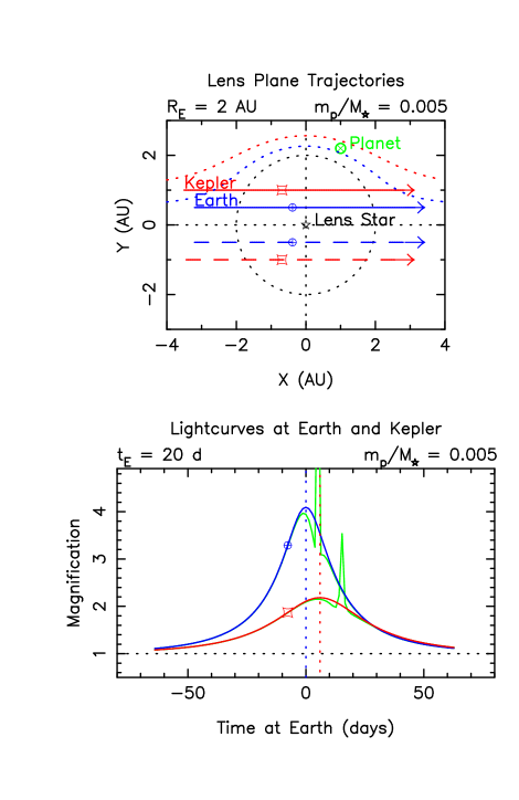
Figure 2: Illustration of four-fold degeneracy derived from comparison of Kepler and ground based lightcurves. Upper panel shows two possible trajectories of the source relative to the lens for each of Kepler (red) and Earth (blue) observatories. Each set would give rise to the same point-lens lightcurve in the lower panel (same colors), leading to an ambiguity in the Earth-Kepler separation (distance between red circle and blue square) relative to the Einstein ring. In this particular case, the planet causes deviations to both lightcurves (green), thus proving that the trajectories are on the same side of the Einstein ring. More generally, the planet would appear in only one curve, leaving the ambiguity open. In this case, it would be resolved by more subtle differences in the Einstein timescale. See Figure 4, below.

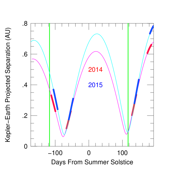
Figure 3: Kepler-Earth projected separation in 2014 (magenta line) and 2015 (cyan line) for Galactic Bulge observations. Red and Blue points show the times when the boresight can be pointed $\pm 45^{\circ}$ and $\pm 90^{\circ}$ from the Sun with the field center still contained within the field of view. Green vertical lines show the approximate boundaries of the microlensing season from Earth.

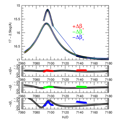
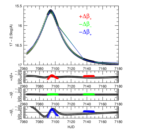
Figure 4: Parallax measurement and degeneracy-breaking for a typical Disk-lens event $(\pi_{{\rm E},N},\pi_{{\rm E},E})=(0.3,0.3)$ (left) and Bulge-lens event $(\pi_{{\rm E},N},\pi_{{\rm E},E})=(0.03,0.03)$ (right). Top panels: Kepler measurements (triangles) over two 14-day windows and Earth measurements (circles) over much longer timescale both shown on arbitrary magnitude scale. Three different models are shown for each, indicated at right in different colors. (In this panel the model curves overlap and can barely be distinguished). The true model is $+\Delta\beta_{-}$, i.e., lens passes the source on its right as seen from Earth (+), and Earth/Kepler both see the lens passing the source on the same side (-). The error bars are 0.005 mag per day from the ground and 0.003 mag per day from Kepler. Lower Panels: residuals for each case for Earth (black) and Kepler (colored). Disk (left): $+\Delta\beta_{+}$ would have $\pi_{\rm E}\sim 1.45$ (factor 3.4 too large) but ruled out by $\Delta\chi^{2}=71$; $-\Delta\beta_{-}$ would have $\pi_{\rm E}\sim 0.44$ (just 5% too large) and is ruled out by ($\Delta\chi^{2}=124$). $-\Delta\beta_{+}$ would have $\pi_{\rm E}\sim 1.13$ (factor 2.7 too large) and ruled out by $\Delta\chi^{2}=2084$. Bulge (right): $+\Delta\beta_{+}$ would have $\pi_{\rm E}\sim 1.6$ (factor 38 too large) but ruled out by $\Delta\chi^{2}=147$; $-\Delta\beta_{-}$ would have $\pi_{\rm E}\sim 0.048$. This is permitted ($\Delta\chi^{2}=1$) but it is just 14% too large; $-\Delta\beta_{+}$ would have $\pi_{\rm E}\sim 1.13$ (factor 26 too large) and ruled out by $\Delta\chi^{2}=1729$.

References

- Choi et al. (2013) Choi, J.-Y., Han, C., Udalski, A., et al. 2013, ApJ, 768, 129
- Dong et al. (2007) Dong, S., Udalski, A., Gould, A., et al. 2007, ApJ, 664,862
- Gaudi & Gould (1997) Gaudi, B.S. & Gould, A. 1997, ApJ, 477, 152
- Gould (1992) Gould, A. 1992, ApJ, 392, 442
- Gould (1994) Gould, A. 1994, ApJ, 421, L75
- Gould (1995) Gould, A. 1995, ApJ, 441, L21
- Gould (1997) Gould, A. 1997, ApJ, 480, 188
- Gould (1999) Gould, A. 1999, ApJ, 514, 869
- Gould (2004) Gould, A. 2004, ApJ, 606, 319
- Gould & Yee (2013) Gould, A. & Yee, J.C. 2013, ApJ, 767, 42
- Hog et al. (1995) Hog, E., Novikov, I.D., & Polanarev, A.G. 1995, A&A, 294, 287
- Miyamoto & Yoshii (1995) Miyamoto, M. & Yoshii, Y. 1995, AJ, 110, 1427
- Refsdal (1966) Refsdal, S. 1966, MNRAS, 134, 315
- Shin et al. (2011) Shin, I.-G., Udalski, A., Han, C. et al. 2011, ApJ, 735, 85
- Shin et al. (2012) Shin, I.-G., Han, C., Choi, J.-Y. et al. 2012, ApJ, 755, 91
- Walker (1995) Walker, M.A. 1995, ApJ, 453, 37
- Yoo et al. (2004) Yoo, J., et al. 2004, ApJ, 603, 139