Optimal Sensor Placement and
Enhanced Sparsity for Classification
Abstract
The goal of compressive sensing is efficient reconstruction of data from few measurements, sometimes leading to a categorical decision.
If only classification is required, reconstruction can be circumvented and the measurements needed are orders-of-magnitude sparser still.
We define enhanced sparsity as the reduction in number of measurements required for classification over reconstruction.
In this work, we exploit enhanced sparsity and learn spatial sensor locations that optimally inform a categorical decision.
The algorithm solves an minimization to find the fewest entries of the full measurement vector that exactly reconstruct the discriminant vector in feature space.
Once the sensor locations have been identified from the training data, subsequent test samples are classified with remarkable efficiency, achieving performance comparable to that obtained by discrimination using the full image.
Sensor locations may be learned from full images, or from a random subsample of pixels.
For classification between more than two categories, we introduce a coupling parameter whose value tunes the number of sensors selected, trading accuracy for economy.
We demonstrate the algorithm on example datasets from image recognition using PCA for feature extraction and LDA for discrimination; however, the method can be broadly applied to non-image data and adapted to work with other methods for feature extraction and discrimination.
Index Terms– Optimal Sensor Placement, Classification, Compressive Sensing, -Minimization, Enhanced Sparsity, Feature Extraction, Face Recognition.
E-mail address: bbrunton@uw.edu (B.W. Brunton).
I Introduction
Classification and detection based on measurements is a crucial capability for intelligent systems, both biological and engineered. It is desirable to perform such categorical tasks with limited or incomplete information, as the full state of the system may be inaccessible or expensive to measure. Fortunately, even when full measurement space is quite high-dimensional, the desired information extracted from the signal is often inherently low-dimensional. For example, images may have a large number of pixels, but it is observed that natural images occupy a minuscule fraction of pixel space. Such an inherent sparsity in an appropriate transformed basis is the foundation of image compression [13]; natural images may be compressed in generic Fourier or wavelet bases.
The theory of compressive sensing [6, 10, 1, 39] takes further advantage of a signal’s compressibility and demonstrates how a -dimensional signal that is -sparse in a transformed basis may be reconstructed exactly from measurements. Here, -sparse means all but coefficients are zero, and we assume . The signal may be reconstructed from the known basis as an -minimal set of sparse coefficients that best recover the measurements. The implementation of compressive sensing rests on the fact that the -minimal solution to an underdetermined linear system may almost certainly be found by relaxation to a convex minimization [6, 10], or by a greedy algorithm [39].
The compressive sensing strategy relies on the measurements being incoherent with respect to the known basis, so that measurement vectors are uncorrelated with basis directions. Incoherence holds between many pairs of bases, such as between delta functions and the Fourier basis. Therefore, it is possible to reconstruct images, which are sparse in the Fourier domain, from single pixel measurements, which may be viewed as discrete spatial delta functions. Surprisingly, a random Gaussian or Bernoulli matrix is incoherent with respect to any arbitrary basis with high probability [6, 10].
Compressive sensing is able to reconstruct a signal using surprisingly few measurements, but assigning a signal to one of a few categories may be accomplished with orders-of-magnitude fewer measurements (for instance, [43]). Typical natural images with pixels can be recovered with significant savings, usually from to measurements [34]. For a 1-megapixel image, this means solving an minimization with constraints in a basis with one million vectors—a non-trivial computational task. In contrast, as we will see, to classify a natural image, only tens of measurement may be required.
Classification is often performed in a tailored low-dimensional basis extracted as hierarchical features of the data. One of the most ubiquitous methods in dimensionality reduction is principal components analysis (PCA) [30, 12], which may be computed by a singular value decomposition (SVD) to yield an ordered orthonormal basis. Linear discriminant analysis (LDA) [3, 14, 33] is commonly applied in conjunction with PCA for discrimination tasks. Indeed, PCA-LDA is one of the classic approaches used to introduce machine learning methodologies [12]. High-variance PCA modes can account for common features shared across categories, which are not useful for discrimination. LDA produces a basis built with respect to the category geometry to maximize between-class variance while minimizing within-class variance. PCA and LDA have both been used extensively for facial recognition (for instance, [36, 41, 37, 2, 45, 28]) and is a benchmark against which novel classification techniques are often compared.
Compared to signal reconstruction, classification is particularly efficient because of 1) the use of a tailored low-dimensional feature basis, and 2) the simplicity of deciding on a category rather than reconstructing exact details [23].
I-A Previous work on enhanced sparsity for classification
Combining ideas from compressive sensing with classification, there has been significant work relevant to exploring enhanced sparsity for classification. For example, the sparse representation algorithm has been applied to biometric recognition problems and demonstrated to be surprisingly robust [43, 31]. Sparse approximation applied to semantic hierarchies [27] has been shown to be efficient in categorizing between large numbers of classes [22]. In another line of work, ideas from compressive sensing have been applied to dimensionality reduction tools to develop a theory of sketched SVD based on randomly projected data [15, 32, 19].
Particularly pertinent to our work is the sparse representation for classification (SRC) algorithm as originally proposed for face recognition by Wright et al. [43]. In SRC, minimization is used to find the sparsest representation of a test image in a dictionary composed of the training images. Each test image is then classified based on the category of dictionary elements whose sparse coefficients best reconstructs the test image, minimizing the residual in an sense. Notably, in this framework, the classification is robust even using dictionaries of tens or hundreds of random projections measurements, due to the enhanced sparsity of classification.
These existing algorithms have all relied on random measurements, typically using dense or sparse random measurement matrices [18]. It remains unexplored how a refinement process may select an optimal subset of measurements to accomplish the classification, further enhancing sparsity. Moreover, acquiring randomly projected measurements may be impractical where many individual point measurements are prohibitively expensive (e.g., ocean or atmospheric sensors). How can classification be accomplished with very few point measurements, and would the locations of those measurements illuminate coherent features of the data?
I-B Contributions and perspectives of this work
In this work, we describe a novel framework to harness the enhanced sparsity in image recognition to classify images based on very few pixel measurements. Its distinct contribution consists of optimally selecting, within a large set of measurement locations, a smaller subset of key locations that serve the classification. We demonstrate that classification using very few learned pixel sensors performs comparably with using the full image. Further, the algorithm includes a parameter to tune the trade-off between fewer sensors and accuracy.
Datasets may be vast and data acquisition can be limited by bandwidth on data streams. Therefore, we also develop an intermediate technique, related to the sketched SVD [15, 18, 19], to start instead with a subsample of the original data. We demonstrate that starting with of the original data, we are still able to find nearly optimal sparse sensor locations.
In generic applications, this entire theory is identical if single pixels are replaced with random projection measurements. In the case of images, the use of single pixel measurements has a number of practical advantages, since pixels are the basic unit of measurement in images. Note that sampling with single-pixel measurements is effective when the image features are non-localized, so that measurements and basis are incoherent. Importantly, sparse sensor pixels identified by our algorithm cluster near coherent features in the images.
Our framework for sparse classification has two characteristics that distinguish it significantly from previous work: 1) instead of random measurements, spatial sensor locations are specifically selected; and 2) minimization is applied once in sensor learning, and classification of new images involves dot products on a very small measurement vector. A schematic representation of our procedure is found in Fig. 1 with details following in the text. Equations (7) and (9) comprise our primary theoretical contributions; Figs. 2 and 7 illustrate the sensor locations produced by the algorithm.
This work takes an engineering perspective of probing complex systems with underlying low-dimensional structure, with the explicit goal of forming some categorical decision about the state of the system. The optimally sparse spatial sensors framework is particularly well suited for engineering applications, as an upfront investment in the learning phase allows remarkably efficient performance for all subsequent queries. Abstractions of this method to more general data sets is discussed in more detail in Sec. V.
We speculate that the principle of enhanced sparsity may also have relevance for biological organisms, which often need to make decisions based on very limited sensory information. Specifically, organisms interact with high-dimensional physical systems in nature but must rely on information gathered through a handful of sensory organs. Our sparse sensor algorithm provides one approach to answer the question, Given a fixed budget of sensors, where should they be placed to optimally inform decision-making?
I-C Organization of the paper
Section II provides an overview of well-known techniques on which we build our contributions and establishes the notation used for the remainder of the paper. We summarize compressive sensing, random projections for matrix decomposition, sparse representation for classification, and the PCA-LDA method for categorization. Section III describes our algorithm for determining optimally sparse sensor locations by using minimization and a dictionary of learned features. We applied sensor learning to two image discrimination tasks based on real-world data; the results of these experiments are presented in Sec. IV and the methods are discussed more generally in Sec. V.
II Background
The main contributions of this work are 1) to design optimal sensor locations that take advantage of enhanced sparsity in classification, and 2) to design sensors from substantially sub-sampled data. To put our contributions in context, we review well known results from compressive sensing in Sec. II-A, which describes the theory of reconstruction, sparse random projection matrices, and sparse representation for classification.
We also make use of two well-established methods for systematically producing low-rank representations of a high-dimensional data set, principal components analysis (PCA) and linear discriminant analysis (LDA). In this manuscript, we demonstrate our algorithm by applying PCA in combination with LDA for face recognition. In general, the method can be implemented with many other dimensionality-reduction and discrimination algorithms, as drawn schematically in the top of Fig. 1. Section II-B reviews PCA-LDA and establishes the notation used to describe our methods in Sec. III.
II-A Compressive sensing and sparse representation
Compressive sensing theory states that if the information of a signal is -sparse in a transformed basis (all but coefficients are zero) and , it is possible to reconstruct the signal from very limited measurements [4, 6, 9, 5]. This technique has widespread applications, including the fields of medical imaging [26], neuroscience [16], and engineering [20].
The standard framing of the compressive sensing problem is as follows. Let us suppose the measurement vector is related to the desired signal by , a known measurement matrix: . Compressive sensing seeks to recover from and applies to the underdetermined case where .
The signal has coefficients in basis , so that
| (1) |
If is sufficiently sparse in and the matrix obeys the restricted isometry principle (RIP) [7], the search for (and thus the reconstruction of ) is possible.
We would like to solve for the sparsest ,
| (2) |
but this involves an intractable combinatorial search. It has been shown that under certain conditions, Eq. (2) may be solved by minimizing the norm [6, 11],
| (3) |
Relaxation to a convex minimization bypasses the combinatorially difficult problem. Solutions to Eq. (3) may be found through standard convex optimization routines, or by greedy algorithms such as orthogonal matching pursuit [40, 39].
An important aspect of compressive sensing is the choice of the measurement matrix . To achieve exact reconstruction, must be incoherent with respect to (therefore satisfying the RIP). Many authors describe the properties of random matrix ensembles that fulfill these conditions with high probability: they include Gaussian, Bernoulli, and random partial Fourier matrices [4, 8, 10]. In addition, sparse random matrices, where many of the entries of the measurement vectors are zero, also allow reconstruction (as reviewed in [18]). Theoretical limits of how sparse random projections may be and still support signal recovery have been explored [25, 42].
In addition to the random measurement framework for reconstruction, we are concerned with the related question of the spectral properties of a data matrix under random projection. Consider a data matrix . Let
where and , as above. Spectral properties of and are approximately equal when the random measurement matrix satisfies the distributed Johnson-Lindenstrauss (JL) property [21, 19]. This property regards the preservation of relative distances between points after random projection to a new space. Since the classification task depends on a geometric separation of data points between classes, the JL property is integral to the success of this model reduction step (dashed arrow between the full and subsampled PCA feature spaces in Fig. 1).
A related line of work on sparse representation for classification (SRC) [43] proposes to leverage sparsity promotion by minimization for image recognition. In this formulation of the classification problem, each training image makes up a column of the dictionary , and the test image is represented as a linear combination of the dictionary elements weighted by coefficients . Thus posed, the solution to the following equation is the sparsest representation of the test image given the dictionary,
Note that the above equation is identical to Eq. (3).
It is then possible to construct a sparse approximation of using only coefficients in associated with the th class,
where is a vector the same size as whose only non-zero entries are the entries in associated with training images in class . Finally, is assigned a category based on the class whose approximation minimizes the residual between and :
The SRC framework exploits enhanced sparsity for classification, making use of the sparse subspace structure of face images. It has been demonstrated to work exceptionally well for many possible dictionaries , including common features such as eigenfaces and Fisher faces, and unncommon features including downsampled faces and random projections.
It is worth noting that the performance of SRC for face recognition is achieved at the cost of one minimization for each test image. As we will see in Sec. III, this is distinct from our algorithm, which uses minimization to identify sparse sensor locations in the training phase only.
II-B PCA, LDA, and classification
Here we describe the two main dimensionality reduction techniques used in this manuscript to demonstrate the pixel refinement algorithm in Sec. III. Consider a set of observations , , where ; also suppose that . Let us construct a data matrix with columns , as represented schematically in Fig. 1; we assume that rows of have been mean subtracted. The PCA consists of performing a singular value decomposition (SVD) defined by the following modal decomposition:
| (4) |
The columns of are the left singular vectors of ; they span the columns of and are often referred to as the principal components or features of the data set. The matrix is diagonal; entries are the singular values of . There are only non-zero singular values, and we may write .
The columns of the matrix are eigenvectors of :
However, this is an extremely expensive eigendecomposition, since the dimension of is . In implementation, it is more practical to use the method of snapshots [35], whereby we solve the eigendecomposition for :
We may then obtain the non-zero PCA modes by taking a linear combination of the columns of :
The SVD provides a systematic approach to transform data into a lower-dimensional representation. For data sets that are inherently low-rank, the singular values of Eq. (4) contains many entries that are exactly zero. With most realistic applications and data sets, though, the singular values often exhibit a power-law decrease, where the low-rank representation of the data is approximate. A power-law decrease of singular values provides an opportunity for a heuristic, and at least quantitatively informed, decision about the number of information-rich dimensions to retain for the reduced-order subspace. Taking the columns of as basis vectors corresponding to the largest singular values, a truncated basis can be formed. We may use this basis to project data from the full measurement space into the reduced -dimensional PCA space (known as feature space):
| (5) | ||||
Thus, the principal components minimize the projection error, .
For categorical decisions, we apply the well known classifier linear discriminant analysis (LDA) in -dimensional feature space. Despite the plethora of classifier techniques, we chose LDA for its simplicity and well-established behavior. We note once again that PCA and LDA are serving only to illustrate the concept proposed in Fig. 1.
We start by noting that each observation (and thus each ) belongs to one of distinct categories where . LDA attempts to find a set of directions in feature space where the between-class variance is maximized and within-class variance is minimized. Specifically,
| (6) |
Here is the within-class scatter matrix,
where is the mean of class . is the between-class scatter matrix,
where is the number of observations in class and is the mean of all observations in (in this case ).
It follows that are eigenvectors corresponding to the non-zero eigenvalues of . It should be noted that the number of non-trivial LDA directions must be less than or equal to the number of categories minus one (), and that at least samples are needed to guarantee is not singular [3].
In schematic form, the top “full image” row of Fig. 1 illustrates the PCA-LDA process for the classification task. In the case of categories, the LDA projection is , and we may apply a threshold value that separates the two categories. Assuming the two categories have equal covariances, we pick the threshold to be the midpoint between the means of the two classes, and .
For decisions between categories, LDA produces a projection . We use a nearest centroid (NC) method for classification, in which a new measurement is assigned to category for which the distance between and is minimal. Many other classifier choices are possible in the reduced space, including nearest neighbor (NN) [12], nearest subspace (NS) [24], support vector machines (SVM) [29], and sparse representation (SRC) [43]. While it is possible these classifiers may improve the accuracy of the decision, we restricted our attention to NC since the focus of this work is not on the specific decision algorithm, but rather on the method of learning sensor locations.
| \begin{overpic}[width=162.6075pt]{chi_and_sensor_placement_line} \put(-2.0,95.0){(a)} \put(50.0,0.0){pixels} \put(17.0,80.0){$\boldsymbol{\chi}$} \put(81.0,80.0){\color[rgb]{1,0,0} $\mathbf{s}$} \end{overpic} | \begin{overpic}[width=162.6075pt]{chi_and_sensor_placement_image.jpeg} \put(3.0,95.0){(b)} \end{overpic} |
III Obtaining sparse sensor locations
This section describes our method to learn sparse sensor locations, building upon the theory described in Sec. II. We begin in Sec. III-A by addressing classification between categories, reducing a full measurement vector to a small handful of key measurements. Section III-B describes an intermediate technique that starts instead with a random subsample of the full data. In Sec. III-C we develop an extension of the algorithm to classification between categories. This subsection also introduces a coupling weight , which allows us to decrease the number of sensors required at the cost of slightly lower classification accuracy. Finally, Sec. III-D demonstrates the possibility of transforming the full-dimensional feature/discrimination projection into an approximate projection from the learned sparse measurements to the decision space. Alternatively, it is possible to re-compute a new projection to decision space directly from the data matrix comprised of sparse measurements, as in the last row of Fig. 1.
In the following, we refer to features (e.g., PCA modes) and discrimination vectors (e.g., LDA directions) to emphasize the generality of the method.
III-A Deciding between two categories
Let us first consider learning sparse sensors for a classification problem between = 2 categories. The discrimination vector encodes the direction in that is most informative in discriminating between categories of observations given by . We seek a measurement vector that satisfies .
In particular, we seek the sparse solution : to find the measurements that best reconstruct , our approach is to solve for
| (7) |
The equations for are under constrained, so that we may use minimization to find the sparse solution to this convex problem. As we will show in Sec. IV, the solution for has at most nonzero elements. Alternatively, it is possible to solve Eq. (7) for exactly nonzero elements using a greedy algorithm [39].
It is important to remember that and can be visualized as an image where most of the pixels are zero. The non-zero elements of represent locations of sensors that best recapture the discriminant projection vector .
To motivate this approach, consider that we have constructed a projection onto a set of features and a projection from feature space to decision space; we may simplify this into a single projection:
where . Therefore, Eq. (7) finds the sparse measurement vector that projects to the same feature space coordinates as :
Finally, we see that
| (8) |
where . That is to say, the sparse measurement is the same as the vector plus some residual vector that does not contain any dominant features (i.e., is not in the span of dominant features).
To compare and , Fig. 2 visualizes these vectors for the dog/cat face recognition problem discussed in Sec. IV-A. Figure 2 (a) shows the magnitude for along with the 20 pixel measurement vector obtained by minimization of Eq. (7). The image of (grey) and the sparse pixels (red) are shown in Fig. 2 (b). Importantly, it is not possible to obtain sparse pixel measurements by thresholding (Fig. 2 (a)); rather, is a sparse image that exactly projects to in space.
To implement this optimal sub-sampling at learned sensors locations, we construct a projection matrix that maps . The number of sensors is usually equal to . The matrix are rows of the identity matrix corresponding to the non-zero elements of .
III-B Learning from randomly subsampled data
The identical approach applies when starting from sub-sampled data (the middle “sub-sampled” row of Fig. 1). We now solve for that best reconstructs the vector in a space defined by the columns of . is then refined to construct , the rows of the identity matrix corresponding to non-zero elements of .
Note that and are both matrices, where typically . Although the two sub-sampling matrices are not the same, we show that in Sec. IV that they are quite similar when .
III-C Deciding between more than two categories
The simplest extension to classification between categories can be implemented by considering the projection to decision space, followed by independently solving Eq. (7) for each column of . However, this approach scales badly with ; in general, discriminating categories of data by projection into -dimensional feature space results in at most learned sensors locations.
An alternative formulation of the convex optimization problem solves for columns of simultaneously; each column of (image) projects to a column of (discrimination vector) in feature space. We introduce a norm that penalizes the total number of non-zero rows in (pixel measurements) to reconstruct the columns of . Specifically,
| (9) |
where , is a column vector of ones, is the Frobenius norm, and is a small error tolerance ( for examples in Sec. IV).
Once again, we have an underdetermined system of equations for . The value of the coupling weight determines the number of non-zero rows of , so that the number of sensors identified is at most where .
In the limit where , the solution to Eq. (9) is the same as obtained by the uncoupled, independent approach. In general, solving Eq. 9 with would result in at most sensor locations. As becomes larger, the coupling between columns of becomes stronger, and the same pixel location can be shared between columns of to approximately reconstruct columns of . In other words, the same pixel measurement is re-used to capture multiple linear discriminant projection vectors. In the limit , the number of sensors is bounded .
The optimization problem as formulated in Eq. (9) is closely related to the one solved by Simultaneous Orthogonal Matching Pursuit (S-OMP, [40, 38]). S-OMP is a greedy algorithm, so instead of a coupling weight parameter , one would decide on a stopping criterion (for example, the desired number of iterations/sensors).
Following the same approach as in deciding between two categories, we implement sub-sampling at learned sensors to construct a projection matrix .
III-D Projecting sparse measurements to classification space
In the above procedure, the projections from the high-dimensional space into feature space () and then into decision space () are computed as a one-time upfront cost. It is then possible to re-use these projections to obtain an induced projection into the decision space starting only from learned sparse measurements. The alternative is to re-compute the discrimination vectors on the sparse measurement data .
Given a new image , we obtain a vector of decision space coordinates as follows:
| (10) |
We then substitute and , where , into Eq. (10):
| (11) |
where . Define as the measurement projection of , so that and . Substituting into Eq. (11) yields:
The matrix defines a new inner-product on the space of sparse measurements that preserves the geometry of decision space. To compute efficiently, compute and separately and then multiply the results.
The alternative approach of re-computing the discrimination projection on the sparse data is typically inexpensive because of the small number of rows. Additionally, for multi-way classification, this usually leads to better performance, as discussed in Sec. IV.
IV Experiments
We apply the algorithm for learning sparse sensor locations, as describe in Sec. III, on two examples of face recognition based on publicly available image datasets. Both data sets are presented and described in Appendix LABEL:app:datasets. In each experiment, we demonstrate that a classifier built on a few optimally placed sparse sensors performs comparably to a classifier built on PCA features of the full image. Moreover, approximately optimal sparse sensor locations may be learned from pixels randomly subsampled from 10% of the full image. Ensembles of the learned sensors cluster at locations consistent with the coherent features in the faces.
IV-A Experiment 1 – Cats and Dogs
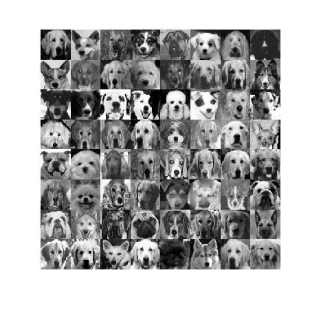
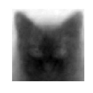
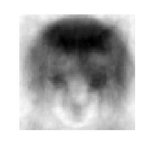
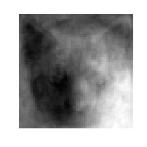
Our first example seeks to classify images of cats versus images of dogs. Each image belongs to a distinct species, and there is considerable variability between individuals of the same species (Fig. 10). Notably, members of each species take on a large range of colorations in fur, markings, and ear postures. We used 121 images each of cats and dogs; images have pixels and are stacked into columns of . Figure 10 (b) shows the first four PCA modes of .
We compared classification accuracy using learned measurements as well as using the principal components of the full image and using random pixel measurements. The accuracy for all of these methods improved with larger numbers of sensors/features; learned sensors performed almost as well as principal components and consistently better than random pixel sensors. Figure 3 shows the results of experiments where classifiers were trained on a random 90% of the images and assessed on the remaining 10% of images. The mean and standard deviation of the cross-validated accuracy over 400 random iterations of training/test images are plotted. Classifiers built on less than 1% of the total pixels (green and red lines in Fig. 3 (a)) performed nearly as well as projections to principal components of the full image.
Accuracy reached a plateau at around features/sensors (Fig. 3 (b)) of around 80%, suggesting the discriminant vector between cats and dogs may be over-fit when more than 15 features were used. Figure 3 (b) shows mean classification performance using sensors learned from subsampled measurements and features, where and are varied systematically. Sparse sensors learned from pixels did almost as well as those learned from pixels. In other words, we were able to learn a nearly optimally sparse set of sensors starting from an already massively under-sampled set of pixels.
The performance of all of these approaches is limited by the large variability in appearances within the categories of cats and dogs. In fact, the images that are most often mis-classified include animals that are predominantly one color (black or white) and dogs with pointy as opposed to droopy ears. In other words, some dog images may not lie close to the bulk of the other dog images in feature space, so that a linear classifier is not able to capture the complex geometry separating the two categories.
It is possible to build classifiers from random pixels that perform significantly better than chance. The improvement in accuracy of using computed features or learned sensors over random pixels became smaller as increases (Fig. 3 (a)). The perhaps surprising performance of random pixels is consistent with the notion of enhanced sparsity and Wright et al.’s [43] observation that using random features, as long as there is enough of them, serves classification as well as using engineered features.
If the sparse sensors represent pixels that are key to the decision, then they should be clustered at locations that are maximally informative about the difference between cats and dogs. Indeed, an average of sensor locations learned over 400 random iterations shows clustering around the animals’ mouth, forehead, eyes, and tops of ears (Fig. 4 (a)). When sparse sensors were learned from an already subsampled dataset, a qualitatively similar distribution of sensor locations was found, where each cluster of sensors showed a slightly larger spatial variance (Fig. 4 (b)). Such an ensemble of sensor placements can be thought of as a mask for facial features particularly relevant for the classification.
Our algorithm applies equally well when the subsampled dataset (middle row in Fig. 1) is not a set of random pixels but a set of random projections. Figure 5 shows that classifiers built on sensors learned from pixels or random projections perform identically. Random projections used to produce this result comprised of ensembles of Bernoulli random variables with mean of 0.5. Even so, Fig. 4 (c) makes clear that using random projections instead of pixels is a poor engineering choice. The ensemble of sensors computed from random projections does not illuminate coherent facial features.
IV-B Experiment 2 – Yale B Faces
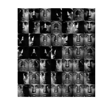
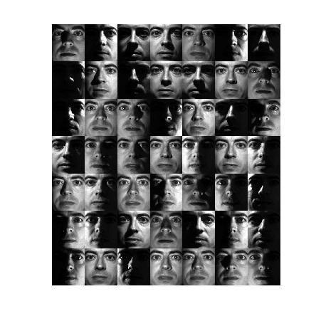
We extended sparse sensor learning to classification between more than two categories, applying our approach to human face recognition. We used the Yale Faces Database B extended [17, 24], which contains images of individual faces captured under various lighting conditions (example images in Fig. 11 (a)). Images have been perviously aligned and cropped; each has pixels. Figure 11 (b) shows the first six eigenfaces corresponding to the three example sets of faces. Comparing the faces dataset with the cat/dog dataset in Sec. IV-A, there is significantly less variability within each category in facial features, although large portions of the faces were effectively occluded by lack of illumination.
We demonstrated our sensor learning approach to learn sensor locations that categorize 3, 4, and 5 faces and compared the classification accuracy of learned sensors to projections to PCA features of the full image and to random sensors of the same number. Figure 6 shows that, as the coupling weight is increased, the number of learned sensors decreases. When , an upper bound of pixels locations were found. In the limit , the number of sensors were bounded by , the number of PCA features included in the discrimination. By adjusting the magnitude of , we gain control over the number of sensor locations used in the classification. When individual sensors are expensive, it may be desirable to use fewer sensors at the cost of slightly lower performance.
The cross-validated accuracy shown in the bottom row of Fig. 6 are results obtained from re-computing the LDA projection to decision space after learning the sensor locations. This strategy is not typically an expensive computation, as the number of rows in the measurement vectors is small. Further, a LDA classifier tailor-made for the specific learned pixels can out-perform the PCA approach when the number of sensors exceeds the number of PCA features. In contrast, the induced projection method described in Sec. III-D cannot perform better than the PCA-LDA approach. For classification between categories, especially for larger coupling weights, re-computing the LDA projection usually leads to more accurate results.
Interestingly, sensors learned from randomly subsampled pixels (10% of the original pixels) performed exactly as well as sensors learned from the full image (red and green lines in Fig. 6). Obtaining sparse sensors from already subsampled data presents significant savings in the learning procedure, both in the SVD to extract a feature space and in the convex optimization to solve for a sparse .
Figure 7 illustrates an example of increasing on the number and locations of sensors identified by the solution to the optimization in Eq. (9). For this example, faces were in the training set so and each has columns. When , the columns of (linear discriminant vectors in dimensional PCA feature space) are treated independently, and total sensors are found. Notice, however, in Fig. 7 (a) that certain pairs of sensor locations are in close proximity (red boxes) and likely carry information about the same non-local facial feature. As increases and the total number of sensors is penalized, these sensor pairs appear to collapse onto single sensors in Fig. 7 (b). Comparing the two sets of sensor locations, we can see that, in additional to aggregated sensors, some sensors have remained the same (for example, the tops of each eyebrow), some sensors have disappeared (on the cheek, at bottom right), while some entirely new sensors have appeared (lower right corner of eye).
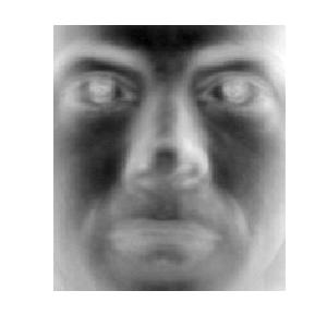
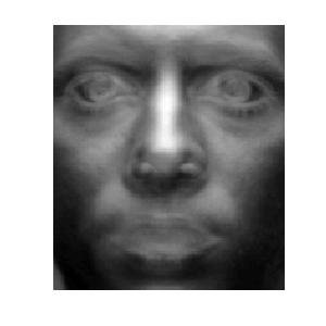
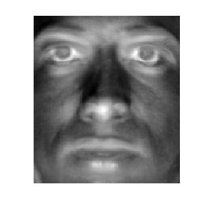
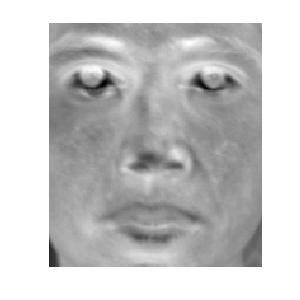
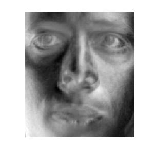
Sparse sensors for face recognition cluster at major facial features: the eyes, the nose, and corners of the mouth (Fig. 8). The nose is particularly prominent in these masks, consistent with the fact that, due to the eccentricity in illumination, the nose is the only facial feature reliably visible in all images. Interestingly, this data-driven algorithm identifies the same features that are favored by humans. As first noted by Yarbus [44], humans examining an image of a face spend a preponderance of time fixating at the eyes, the nose, and the mouth.
| \begin{overpic}[width=104.07117pt]{sensor_locations_3faces.jpeg} \put(0.0,90.0){(a)} \put(29.0,96.0){mean sensors} \end{overpic} | \begin{overpic}[width=104.07117pt]{sensor_locations_mean_face1.jpeg} \put(0.0,90.0){(b)} \put(29.0,96.0){mean face 1} \end{overpic} |
| \begin{overpic}[width=104.07117pt]{sensor_locations_mean_face2.jpeg} \put(0.0,90.0){(c)} \put(29.0,96.0){mean face 2} \end{overpic} | \begin{overpic}[width=104.07117pt]{sensor_locations_mean_face3.jpeg} \put(0.0,90.0){(d)} \put(29.0,96.0){mean face 3} \end{overpic} |
V Discussion
In this paper, we described an algorithm that refines a large set of measurement locations to learn a much smaller subset of key locations to best serve a classification task. Steps of the algorithm are shown in Fig. 9. The algorithm exploits enhanced sparsity for classification, when reconstruction may be bypassed. Enhanced sparsity provides an orders-of-magnitude reduction in number of measurements required when compared with standard compressive sensing strategies. Measurements are projected directly into decision space; reconstruction from so few measurements is neither possible or needed.
Our algorithm leverages the sparsity promoting minimization as phrased in Eqs. (7) or (9). These convex optimization problems solve for a sparse set of sensor locations to closely approximate the linear discrimination vector in PCA space. The approach may be generalized to a variety of other dimensionality reduction and discrimination algorithms. In addition, once a set of sensors have been obtained, a number of more sophisticated classifier algorithms may be applied to these measurements to improve the classification accuracy.
We demonstrated our approach on two examples of image recognition. Classifiers built on learned sensors approached the performance of classifiers built on projections to principal components of the full images. These optimal sensor locations could be learned approximately even from already randomly subsampled images. In either case, the learned sensors performed significantly better than the matched number of randomly chosen sensors. Further, the ensemble of learned sensor locations clustered around coherent features of the images. It is possible to think of this ensemble as a pixel mask for the faces in the training set, which may be of use when applied to engineered or biological systems where the important features may not be salient by inspection.
It is plausible that biological organisms may exploit enhanced sparsity for classification. Organisms interact with the external world with motor outputs, which are often discrete trajectories at specific moments in time, so that the transformation from sensory inputs to motor outputs can be thought of as a classification task. For example, a fly has no need to reconstruct the full flow velocity field around its body—it has only to decide what to do in response to a gust. Sensory organs and data processing by the nervous system can be expensive; therefore, it is advantageous to place a smaller number of sensors at key locations on the body.
Although introduced for image discrimination, the algorithm may be applied to a variety of non-image data types with more general sensor networks. One such application is the detection of disease spread in epidemiological monitoring. We also envision these methods applying to mobile sensor networks in oceanographic and atmospheric sampling, as well as to detect and monitor various network behaviors in the electrical grid, internet packet routing, and transportation.
Acknowledgements
We especially thank Tom Daniel and Leifeng Bo for helpful discussions related to this work, and Anna Gilbert for insightful comments on the manuscript. B. W. Brunton and J. N. Kutz acknowledge support from the National Science Foundation (DMS-1007621); S. L. Brunton and J. N. Kutz acknowledge support from the U.S. Air Force Office of Scientific Research (FA9550-09-0174). J. L. Proctor acknowledges support by Intellectual Ventures Laboratory.
References
- [1] R. G. Baraniuk. Compressive sensing. IEEE Signal Processing Magazine, 24(4):118–120, 2007.
- [2] P. N. Belhumeur, J. P. Hespanha, and D. J. Kriegman. Eigenfaces vs. Fisherfaces: Recognition using class specific linear projection. IEEE Transactions on Pattern Analysis and Machine Intelligence (PAMI), 19(7):711–720, 1997.
- [3] C. M. Bishop. Pattern recognition and machine learning. Springer, New York, 2006.
- [4] E. J. Candès. Compressive sensing. Proceedings of the International Congress of Mathematics, 2006.
- [5] E. J. Candès, Y. Eldar, D. Needell, and P. Randall. Compressed sensing with coherent and redundant dictionaries. Applied and Computational Harmonic Analysis, 31:59–73, 2010.
- [6] E. J. Candès, J. Romberg, and T. Tao. Robust uncertainty principles: exact signal reconstruction from highly incomplete frequency information. IEEE Transactions on Information Theory, 52(2):489–509, 2006.
- [7] E. J. Candes and T. Tao. Decoding by linear programming. Information Theory, IEEE Transactions on, 51(12):4203–4215, 2005.
- [8] E. J. Candès and T. Tao. Near optimal signal recovery from random projections: Universal encoding strategies? IEEE Transactions on Information Theory, 52(12):5406–5425, 2006.
- [9] E. J. Candès and M. B. Wakin. An introduction to compressive sampling. IEEE Signal Processing Magazine, pages 21–30, 2008.
- [10] D. L. Donoho. Compressed sensing. IEEE Transactions on Information Theory, 52(4):1289–1306, 2006.
- [11] D. L. Donoho. For most large underdetermined systems of linear equations the minimal 𝓁1-norm solution is also the sparsest solution. Communications on pure and applied mathematics, 59(6):797–829, 2006.
- [12] R. O. Duda, P. E. Hart, and D. G. Stork. Pattern Classification. Wiley-Interscience, 2000.
- [13] M Elad. Sparse and redundant representations: from theory to applications in signal and image processing. Springer, New York, 2010.
- [14] R. A. Fisher. The use of multiple measurements in taxonomic problems. Annals of Eugenics, 7(2):179–188, 1936.
- [15] J. E. Fowler. Compressive-projection principal component analysis. IEEE Transactions on Image Processing, 18(10):2230–2242, 2009.
- [16] S. Ganguli and H. Sompolinsky. Compressed sensing, sparsity, and dimensionality in neuronal information processing and data analysis. Annual Review of Neuroscience, 35:485–508, 2012.
- [17] A.S. Georghiades, P.N. Belhumeur, and D.J. Kriegman. From few to many: Illumination cone models for face recognition under variable lighting and pose. Pattern Analysis and Machine Intelligence, IEEE Transactions on, 23(6):643–660, 2001.
- [18] A. C. Gilbert and P. Indyk. Sparse recovery using sparse matrices. Proceedings of the IEEE, 5=98(6):937–947, 2010.
- [19] A. C. Gilbert, J. Y. Park, and M. B. Wakin. Sketched SVD: Recovering spectral features from compressive measurements. ArXiv e-prints, 2012.
- [20] M.A. Herman and T. Strohmer. High-resolution radar via compressed sensing. Signal Processing, IEEE Transactions on, 57(6):2275–2284, 2009.
- [21] W. B Johnson and J. Lindenstrauss. Extensions of lipschitz mappings into a hilbert space. Contemporary mathematics, 26(189-206):1, 1984.
- [22] B. Kim, J. Y. Park, A. Mohan, A. C. Gilbert, and S. Savarese. Hierarchical classification of images by sparse approximation. In BMVC, pages 1–11. Citeseer, 2011.
- [23] J. N. Kutz. Data-Driven Modeling & Scientific Computation: Methods for Complex Systems & Big Data. Oxford University Press, 2013.
- [24] K. Lee, J. Ho, and D. J Kriegman. Acquiring linear subspaces for face recognition under variable lighting. IEEE Trans Pattern Anal Mach Intell, 27(5):684–98, May 2005.
- [25] P. Li, T. J. Hastie, and K. W. Church. Very sparse random projections. In Proceedings of the 12th ACM SIGKDD international conference on Knowledge discovery and data mining, pages 287–296. ACM, 2006.
- [26] M. Lustig, D.L. Donoho, J.M. Santos, and J.M. Pauly. Compressed sensing mri: A look at how cs can improve on current imaging techniques. IEEE Signal Processing Magazine, 25(2):72–82, 2008.
- [27] M. Marszalek and C. Schmid. Semantic hierarchies for visual object recognition. In Computer Vision and Pattern Recognition, 2007. CVPR’07. IEEE Conference on, pages 1–7. IEEE, 2007.
- [28] A. M. Martinez and A. C. Kak. PCA versus LDA. IEEE Transactions on Pattern Analysis and Machine Intelligence (PAMI), 23(2):228–233, 2001.
- [29] A. Muñoz and J.M. Moguerza. Estimation of high-density regions using one-class neighbor machines. IEEE Trans Pattern Anal Mach Intell, 28(3):476–80, Mar 2006.
- [30] K. Pearson. On lines and planes of closest fit to systems of points in space. Philosophical Magazine, 2(7–12):559–572, 1901.
- [31] J. K. Pillai, V. M Patel, R. Chellappa, and N. K Ratha. Secure and robust iris recognition using random projections and sparse representations. Pattern Analysis and Machine Intelligence, IEEE Transactions on, 33(9):1877–1893, 2011.
- [32] H. Qi and S. M. Hughes. Invariance of principal components under low-dimensional random projection of the data. IEEE International Conference on Image Processing, October 2012.
- [33] C. R. Rao. The utilization of multiple measurements in problems of biological classification. Journal of the Royal Statistical Society. Series B (Methodological), 10(2):159–203, 1948.
- [34] J. Romberg. Imaging via compressive sampling. Signal Processing Magazine, IEEE, 25(2):14–20, 2008.
- [35] L. Sirovich. Turbulence and the dynamics of coherent structures, parts I-III. Q. Appl. Math., XLV(3):561–590, 1987.
- [36] L. Sirovich and M. Kirby. A low-dimensional procedure for the characterization of human faces. Journal of the Optical Society of America A, 4(3):519–524, 1987.
- [37] D. L. Swets and J. Weng. Using discriminant eigenfeatures for image retrieval. IEEE Transactions on Pattern Analysis and Machine Intelligence (PAMI), 18(8):831–836, 1996.
- [38] J. A. Tropp. Algorithms for simultaneous sparse approximation. part ii: Convex relaxation. Signal Processing, 86(3):589–602, 2006.
- [39] J. A. Tropp and A. C. Gilbert. Signal recovery from random measurements via orthogonal matching pursuit. IEEE Transactions on Information Theory, 53(12):4655–4666, 2007.
- [40] J. A. Tropp, A. C. Gilbert, and M. J. Strauss. Algorithms for simultaneous sparse approximation. part i: Greedy pursuit. Signal Processing, 86(3):572–588, 2006.
- [41] M. Turk and A. Pentland. Eigenfaces for recognition. Journal of Cognitive Neuroscience, 3(1):71–86, 1991.
- [42] W. Wang, M.J. Wainwright, and K. Ramchandran. Information-theoretic limits on sparse signal recovery: Dense versus sparse measurement matrices. Information Theory, IEEE Transactions on, 56(6):2967–2979, 2010.
- [43] J. Wright, A. Yang, A. Ganesh, S. Sastry, and Y. Ma. Robust face recognition via sparse representation. IEEE Transactions on Pattern Analysis and Machine Intelligence (PAMI), 31(2):210–227, 2009.
- [44] A.L. Yarbus, B. Haigh, and L.A. Rigss. Eye movements and vision. Plenum press New York, 1967.
- [45] H. Yu and J. Yang. A direct LDA algorithm for high-dimensional data – with application to face recognition. Pattern Recognition, 34:2067–2070, 2001.