High-Order Discontinuous Galerkin Finite Element Methods with Globally Divergence-Free Constrained Transport for Ideal MHD

Abstract

The modification of the celebrated Yee scheme from the vacuum Maxwell equations to magnetohydrodynamics (MHD) is often referred to as the constrained transport (CT) approach. Constrained transport can be viewed as a sort of predictor-corrector method for updating the magnetic field, where a magnetic field value is first predicted by a method that does not exactly preserve the divergence-free condition on the magnetic field, followed by a correction step that aims to control these divergence errors. This strategy has been successfully used in conjunction with a variety of shock-capturing methods including WENO (weighted essentially non-oscillatory), central, and wave propagation schemes. In this work we show how to extend the basic CT framework in the context of the discontinuous Galerkin (DG) finite element method on both 2D and 3D Cartesian grids. We first review the entropy-stability theory for semi-discrete DG discretizations of ideal MHD, which rigorously establishes the need for a magnetic field that satisfies the following conditions: (1) the divergence of the magnetic field is zero on each element, and (2) the normal components of the magnetic field are continuous across all element edges (faces in 3D). In order to achieve such a globally divergence-free magnetic field, we introduce a novel constrained transport scheme that is based on two main ingredients: (1) we introduce an element-centered magnetic vector potential that is updated via a discontinuous Galerkin scheme on the induction equation; and (2) we define a mapping that takes element-centered magnetic field values (i.e., the predicted magnetic field) and element-centered magnetic vector potential values and creates on each edge (face in 3D) a high-order representation of the normal component of the magnetic field; this representation is then mapped back to the elements to create a globally divergence-free element-centered representation of the magnetic field. For problems with shock waves, we make use of so-called moment-based limiters to control oscillations in the conserved quantities. The resulting method is applied to standard test cases for ideal MHD.

1 Introduction

Plasma is often referred to as the fourth state of matter after solid, liquid, and gas, and consists of a mixture of interacting charged particles. Macroscopic features of a quasi-neutral plasma can often be accurately modeled through magnetohydrodynamic (MHD) models that track only macroscopic quantities such as the total mass density, center-of-mass momentum density, and total energy density (see standard plasma physics textbooks such as Chapter 4 of Gombosi [16]). The ideal magnetohydrodynamic equations further assume that the flow is inviscid and that the plasma is a perfect conductor (i.e., zero resistivity).

The ideal MHD system can be written as a system of hyperbolic conservation laws, where the conserved quantities are mass density, momentum density, energy density, and the magnetic field. Furthermore, this system is equipped with an entropy inequality that features a convex scalar entropy and a corresponding entropy flux. Indeed, the scalar entropy, with some help from the fact that the magnetic field is divergence-free, can be used to define entropy variables in which the MHD system is in symmetric hyperbolic form [5, 15].

As has been noted many times in the literature (e.g., Brackbill and Barnes [7], Evans and Hawley [12], and Tóth [36]), numerical methods for ideal MHD must in general satisfy (or at least control) some discrete version of the divergence-free condition on the magnetic field:

$$\nabla\cdot{\bf B}=0.$$ (1)

Failure to accomplish this generically leads to a nonlinear numerical instability, which often leads to negative pressures and/or densities. Starting with the paper of Brackbill and Barnes [7] in 1980, several approaches for controlling errors in $\nabla\cdot{\bf B}$ have been proposed. An in-depth review of many of these methods can be found in Tóth [36].

The constrained transport (CT) approach for ideal MHD was introduced by Evans and Hawley [12]. The method is a modification of Yee’s method [38] for electromagnetic wave propagation, and, at least in its original formulation, introduced staggered magnetic and electric fields. This approach can also be viewed as a kind of predictor-corrector scheme for the magnetic field. Roughly speaking, the idea is to compute all of the conserved quantities with a “standard” finite difference, finite volume, or finite element method. This step produces the predicted magnetic field values. From these computed quantities one then constructs an approximation to the electric field through the ideal Ohm’s law. This electric field can then be used to update the magnetic vector potential, which in turn, can be used to compute a divergence-free magnetic field. This step produces the corrected magnetic field values.

The main advantages of this approach compared to other approaches for solving the ideal MHD equations are that (1) there is no elliptic solve such as in projection methods (e.g., see Tóth [36] and Balsara and Kim [2]), and (2) there are no free parameters to choose such as in the hyperbolic divergence-cleaning technique [11]. The main disadvantages of this approach are that (1) additional variables must be stored and updated (i.e., the magnetic potential), and (2) a staggered description typical of mixed finite element methods is often required.

Since the introduction of the original CT framework by Evans and Hawley [12], several variants and modifications have been introduced, including the work of Balsara [1], Balsara and Spicer [3], Christlieb et al. [8], Dai and Woodward [10], Fey and Torrilhon [13], Helzel et al. [20, 21], Londrillo and Del Zanna [26], Rossmanith [32], Ryu et al. [34], and De Sterck [35]. An overview of many of these approaches, as well as the introduction of a few more variants, can be found in Tóth [36].

In this work we show how to extend the basic constrained transport framework in the context of the discontinuous Galerkin finite element method (DG-FEM) on both 2D and 3D Cartesian meshes. The method advocated in this work makes use of two key ingredients: (1) the introduction of a magnetic vector potential, which in our case will be represented in the same finite element space as the conserved variables, and (2) the use of a particular divergence-free reconstruction of the magnetic field, which makes use of the magnetic vector potential and the predicted magnetic field. The divergence-free reconstruction advocated in this work is slight modification of the reconstruction method that has been used in other work on ideal MHD. Li, Xu, and Yakovlev [25] made use of this reconstruction in the context of a 2D central DG scheme. Balsara [1] made use this reconstruction in the context of finite volume schemes and adaptive mesh refinement. In fact, the divergence-free reconstruction of the magnetic field is directly related to ideas from discrete exterior calculus and, in particular, to Whitney forms (e.g., see Bossavit [6]). Despite these connections, we do need the full machinery of discrete exterior calculus and Whitney forms in order to develop the proposed numerical scheme. The novel aspect of this work is that we make direct use of a magnetic vector potential, thus following in the footsteps of the methods developed in [8, 20, 21, 26, 32, 35]. An advantage of our approach is that extension from 2D to 3D is straightforward.

The paper begins with a description of the ideal MHD equations in §2. In §3 we describe the basic DG method, both on 2D and 3D Cartesian meshes. In §4 we review the entropy stability theory for semi-discrete DG-FEM, including a discussion of the relevant theorem of Barth [5] that rigorously establishes the need for divergence-free magnetic fields in the discretization of MHD. In §5 we introduce a novel constrained transport scheme that is based on achieving a globally divergence-free magnetic field via the use of a combination of techniques from mixed finite element methods, as well as through the use of a magnetic potential. The magnetic potential is updated through an appropriate high-order discretization of the induction equation, and a globally divergence-free magnetic field is then constructed through a discrete curl operation on the magnetic potential. In particular, the discrete curl of the magnetic potential is defined through a high-order construction of the normal components of the magnetic field on each element edge, followed by a reconstruction step to obtain a globally-defined element-centered definition of the magnetic field. This newly proposed method is closely related to the central DG scheme for ideal MHD developed by Li, Xu, and Yakovlev [25], although the new scheme does not require the use of central DG, nor does it require storing the solution on both a primal and a dual grid. For these reasons, extension to 3D is straightforward. The resulting scheme is applied to several numerical test cases in §6. All of the methods presented in this work have been implemented in the DoGPack software package [30] and will be made freely available on the web. All the visualization in this work has been done with the freely available package Matplotlib [22].

2 Ideal magnetohydrodynamic equations

The ideal magnetohydrodynamic (MHD) equations are a classical model from plasma physics that describe the macroscopic evolution of a quasi-neutral two-fluid plasma system. Under the quasi-neutral assumption, the two-fluid equations can be collapsed into a single set of fluid equations for the total mass density, center-of-mass momentum density, and total energy density of the system. The resulting equations can be written in the following form:

$$\frac{\partial}{\partial t}\begin{bmatrix}\rho\\ \rho{\bf u}\\ {\mathcal{E}}\\ {\bf B}\end{bmatrix}+\nabla\cdot\begin{bmatrix}\rho{\bf u}\\ \rho{\bf u}{\bf u}+\left({p}+\frac{1}{2}\|{\bf B}\|^{2}\right){\mathbb{I}}-{\bf B}{\bf B}\\ {\bf u}\left({\mathcal{E}}+{p}+\frac{1}{2}\|{\bf B}\|^{2}\right)-{\bf B}\left({\bf u}\cdot{\bf B}\right)\\ {\bf u}{\bf B}-{\bf B}{\bf u}\end{bmatrix}=0,$$ (2)

$$\nabla\cdot{\bf B}=0,$$ (3)

where $\rho$, $\rho{\bf u}$, and ${\mathcal{E}}$ are the mass, momentum, and energy densities of the plasma system, and ${\bf B}$ is the magnetic field. The thermal pressure, $p$, is related to the conserved quantities through the ideal gas law:

$$p=\left(\gamma-1\right)\left({\mathcal{E}}-\frac{1}{2}\|{\bf B}\|^{2}-\frac{1}{2}\rho\|{\bf u}\|^{2}\right),$$ (4)

where $\gamma=5/3$ is the ideal gas constant.

Note that the equation for the magnetic field comes from Faraday’s law:

$${\bf B}_{,t}+\nabla\times{\bf E}=0,$$ (5)

where the electric field, ${\bf E}$, is approximated by Ohm’s law for a perfect conductor:

$${\bf E}={\bf B}\times{\bf u}.$$ (6)

Since the electric field is determined entirely from Ohm’s law, we do not require an evolution equation for it; and thus, the only other piece that we need from Maxwell’s equations is the divergence-free condition on the magnetic field (3). A complete derivation and discussion of MHD system (2)-(3) can be found in several standard plasma physics textbooks (e.g., pages 69–78 of [16]).

2.1 Hyperbolicity

We first note that system (2), along with the equation of state (4), provides a full set of equations for the time evolution of all eight state variables: $\left(\rho,\,\rho{\bf u},\,{\mathcal{E}},\,{\bf B}\right)$. These evolution equations form a hyperbolic system. In particular, the eigenvalues of the flux Jacobian in some arbitrary direction ${\bf n}$ ($\|{\bf n}\|=1$) can be written as follows:

$$\lambda^{1,8}={\bf u}\cdot{\bf n}\mp c_{f}\quad\text{(fast magnetosonic),}\qquad\lambda^{2,7}={\bf u}\cdot{\bf n}\mp c_{a}\quad\text{(Alfv$\acute{\text{e}}$n),}$$ (7)

$$\lambda^{3,6}={\bf u}\cdot{\bf n}\mp c_{s}\quad\text{(slow magnetosonic),}\qquad\lambda^{4}={\bf u}\cdot{\bf n}\quad\text{(entropy),}\qquad\lambda^{5}={\bf u}\cdot{\bf n}\quad\text{(divergence),}$$ (8)

where

$$a\equiv\sqrt{\frac{\gamma p}{\rho}},\qquad c_{a}\equiv\sqrt{\frac{\left({\bf B}\cdot{\bf n}\right)^{2}}{\rho}},\qquad c_{f},c_{s}\equiv\left\{\frac{1}{2}\left[a^{2}+\frac{\|{\bf B}\|^{2}}{\rho}\pm\sqrt{\left(a^{2}+\frac{\|{\bf B}\|^{2}}{\rho}\right)^{2}-4a^{2}\frac{\left({\bf B}\cdot{\bf n}\right)^{2}}{\rho}}\right]\right\}^{1/2}.$$ (9)

The eigenvalues are well-ordered in the sense that

$$\lambda^{1}\leq\lambda^{2}\leq\lambda^{3}\leq\lambda^{4}\leq\lambda^{5}\leq\lambda^{6}\leq\lambda^{7}\leq\lambda^{8}\,.$$ (10)

The fast and slow magnetosonic waves are genuinely nonlinear, while the remaining waves are linearly degenerate. Note that the so-called divergence-wave has been made to travel at the speed ${\bf u}\cdot{\bf n}$ via the 8-wave formulation, thus restoring Galilean invariance [15, 28, 29]. Also note that despite the fact that we use the eigenvalues and eigenvectors of the 8-wave formulation of the MHD equations, we will still solve the MHD equations in conservative form (i.e., without the “Powell source term”). See §2.3 and §4 for more discussion on this issue.

2.2 Symmetric hyperbolic structure of standard hyperbolic conservation laws

Consider a conservation law in $d$ spatial dimensions with ${M_{\text{eq}}}$ number of conserved variables of the form:

$$q_{,t}+\nabla\cdot{\bf F}(q)=0,\quad\text{in}\quad{\bf x}\in\Omega\subset{{\rm l}\kern-1.49994pt{\rm R}}^{d},$$ (11)

with appropriate initial and boundary conditions. In this equation $q:{{\rm l}\kern-1.49994pt{\rm R}}^{+}\times{{\rm l}\kern-1.49994pt{\rm R}}^{d}\mapsto{{\rm l}\kern-1.49994pt{\rm R}}^{{M_{\text{eq}}}}$ is the vector of conserved variables and ${\bf F}:{{\rm l}\kern-1.49994pt{\rm R}}^{{M_{\text{eq}}}}\mapsto{{\rm l}\kern-1.49994pt{\rm R}}^{{{M_{\text{eq}}}}\times d}$ is the flux function. We assume that equation (11) is hyperbolic, meaning that the family of ${{M_{\text{eq}}}}\times{{M_{\text{eq}}}}$ matrices defined by

$$A(q;{\bf n})=\frac{\partial\left({\bf n}\cdot{\bf F}\right)}{\partial q}$$ (12)

are diagonalizable with real eigenvalues for all $q$ in the domain of interest and for all vectors ${\bf n}$ such that $\|{\bf n}\|=1$. The matrix $A(q;{\bf n})$ in (12) is often referred to as the flux Jacobian.

Many important hyperbolic conservation laws arising in physical applications are equipped with a convex entropy extension that can be used along with appropriate jump conditions to determine what weak solutions of (11) can be considered admissible. Let $U:{{\rm l}\kern-1.49994pt{\rm R}}^{{M_{\text{eq}}}}\mapsto{{\rm l}\kern-1.49994pt{\rm R}}$ and ${\bf G}:{{\rm l}\kern-1.49994pt{\rm R}}^{{M_{\text{eq}}}}\mapsto{{\rm l}\kern-1.49994pt{\rm R}}^{d}$ denote an entropy function and associated entropy flux that satisfy the following entropy inequality:

$$U(q)_{,t}+\nabla\cdot{\bf G}(q)\leq 0,$$ (13)

where $q$ is a weak solution of (11). The definitions of $U$ and ${\bf G}$ are such that inequality (13) becomes an exact equality for classical solutions.

The existence of the above entropy and the associated entropy flux is closely related to the fact that system (11) can in many cases (e.g., shallow water equations, compressible Euler equations, and Euler-Maxwell) be put in symmetric hyperbolic form via a transformation of the dependent variables. In particular, we seek a mapping $q(v)$ from ${{\rm l}\kern-1.49994pt{\rm R}}^{{M_{\text{eq}}}}$ to ${{\rm l}\kern-1.49994pt{\rm R}}^{{M_{\text{eq}}}}$ such that (11) becomes

$$q_{,v}\,v_{,t}+\sum_{\ell=1}^{d}F^{\ell}_{,v}\,\,v_{,x^{\ell}}=0,$$ (14)

where $q_{,v}\in{{\rm l}\kern-1.49994pt{\rm R}}^{{{M_{\text{eq}}}}\times{{M_{\text{eq}}}}}$ is symmetric positive definite and $F^{\ell}_{,v}\in{{\rm l}\kern-1.49994pt{\rm R}}^{{{M_{\text{eq}}}}\times{{M_{\text{eq}}}}}$ is symmetric for all $\ell=1,\ldots,d$. In several important cases it turns out that the symmetrization variables, $v$, are directly related to the entropy function via the relationship:

$$v=U_{,q}.$$ (15)

For more details on the the symmetrization theory for nonlinear hyperbolic conservation laws see for example [14, 27, 37, 19].

2.3 Symmetric hyperbolic structure of ideal MHD

In the case of ideal MHD, a suitable entropy function is the physical entropy density (divided by $\gamma-1$ for convenience):

$$U(q):=-\frac{\rho s}{\gamma-1},$$ (16)

where $s$ is the physical entropy:

$$s:=\log\left(\frac{p}{\rho^{\gamma}}\right).$$ (17)

The minus sign in (16) is there to make sure that the entropy function decreases, which is the usual convention in the theory of hyperbolic conservation laws. Computing the time derivative of the entropy function and using the conservation laws from the MHD system (2) results in the following equation for the entropy function (for smooth solutions):

$$U(q)_{,t}+\nabla\cdot{\bf G}(q)+\chi(q)\left(\nabla\cdot{\bf B}\right)=0,$$ (18)

where

$${\bf G}(q):={\bf u}U\quad\text{and}\quad\chi(q):=\frac{\rho{\bf u}\cdot{\bf B}}{p}.$$ (19)

The key point is that the entropy function is only conserved (for smooth solutions) if the magnetic field is exactly divergence-free: $\nabla\cdot{\bf B}=0$. Since entropy and symmetrization are connected, this result suggests that the involution (3) might play an important role in the symmetrization of the MHD equations. Indeed it does.

The entropy variables are

$$v=U_{,q}=\left[\frac{\gamma-s}{\gamma-1}-\frac{\|{\bf u}\|^{2}}{2T},\,\frac{{\bf u}}{T},\,-\frac{1}{T},\,\frac{{\bf B}}{T}\right]^{T},$$ (20)

where $T=p/\rho$ is the temperature. A straightforward calculation shows that using these variables results in an equation of the form (14), where $q_{,v}\in{{\rm l}\kern-1.49994pt{\rm R}}^{8\times 8}$ is indeed symmetric positive definite, but where the matrices $F^{\ell}_{,v}\in{{\rm l}\kern-1.49994pt{\rm R}}^{8\times 8}$ for $\ell=1,2,3$ are unfortunately not symmetric. This fact was first observed by Godunov [15].

Godunov [15] provided a remedy for this situation, which involved adding to (14) a term that is proportional to $\nabla\cdot{\bf B}$:

$$\begin{split}q_{,v}\,v_{,t}+\sum_{\ell=1}^{d}F^{\ell}_{,v}\,v_{,x^{\ell}}+\chi_{,v}\,\left(\nabla\cdot{\bf B}\right)=0\quad\Longrightarrow\quad q_{,v}\,v_{,t}+\sum_{\ell=1}^{d}\widetilde{A}^{\ell}\,v_{,x^{\ell}}=0,\end{split}$$ (21)

where $\chi$ is defined by (19) and the matrices $\widetilde{A}^{\ell}\in{{\rm l}\kern-1.49994pt{\rm R}}^{8\times 8}$, for $\ell=1,2,3$, are symmetric [5].

The additional term in the above expression is sometimes referred to as the Powell source term [28, 29], since Powell advocated including this term in numerical simulations of MHD (see §4 for much more discussion on this point). The fact that the involution $\nabla\cdot{\bf B}=0$ is needed in order to symmetrize the MHD equations has direct consequences on the stability of numerical discretizations of MHD. We will discuss this in more detail in §4.

We also note the following identities, which will become useful in the DG stability analysis:

$$v\cdot q_{,t} =U_{,t},$$ (22)

$$v\cdot\left(\nabla\cdot{\bf F}\right) =\nabla\cdot{\bf G}-\chi\,\nabla\cdot{\bf B},$$ (23)

$$v\cdot\chi_{,v}\,\nabla\cdot{\bf B} =\chi\,\nabla\cdot{\bf B}.$$ (24)

These identities conspire to produce the following important result in the case of smooth solutions:

$$v\cdot\left\{q_{,t}+\nabla\cdot{\bf F}+\chi_{,v}\,\nabla\cdot{\bf B}\right\}=U_{,t}+\nabla\cdot{\bf G}=0.$$ (25)

In words, this result says that multiplying the augmented MHD equations (i.e., MHD with the “Powell source term”) by the symmetrization variables yields the conservation law for the entropy function. Finally, we introduce the dual entropy and dual entropy flux:

$$U+U^{\star} =v\cdot q \qquad\Longrightarrow\qquad U^{\star} :=\rho+\frac{\|{\bf B}\|^{2}}{2T},$$ (26)

$${\bf G}+{\bf G}^{\star} =v\cdot{\bf F}+\chi\,{\bf B} \qquad\Longrightarrow\qquad{\bf G}^{\star} :=\rho{\bf u}+\frac{{\bf u}\|{\bf B}\|^{2}}{2T},$$ (27)

which satisfy the following relationships:

$$q=U^{\star}_{,v}\qquad\text{and}\qquad{\bf F}={\bf G}^{\star}_{,v}-\chi_{,v}\,{\bf B}.$$ (28)

3 Discontinuous Galerkin finite element methods

The modern form of the discontinuous Galerkin (DG) finite element method for solving hyperbolic PDEs of the form (11) was developed in a series of papers by Bernardo Cockburn, Chi-Wang Shu, and their collaborators (see e.g., [9]). In this section we briefly review the general framework of the DG method in §3.1, and give further details for 2D Cartesian meshes in §3.2 and 3D Cartesian meshes in §3.3. This section also serves to explain the notation used throughout this paper.

3.1 General framework

Let $\Omega\subset{{\rm l}\kern-1.49994pt{\rm R}}^{d}$ be a polygonal domain with boundary $\partial\Omega$. We discretize $\Omega$ using a finite set of non-overlapping elements, ${\mathcal{T}}_{i}$, such that $\Omega=\cup_{i=1}^{N}{\mathcal{T}}_{i}$. Let ${P}^{\,{\text{q}}}\left({{\rm l}\kern-1.49994pt{\rm R}}^{d}\right)$ denote the set of polynomials from ${{\rm l}\kern-1.49994pt{\rm R}}^{d}$ to ${{\rm l}\kern-1.49994pt{\rm R}}$ with maximal polynomial degree q; for example, the polynomial $x^{a}y^{b}z^{c}$, where $a,b,c$ are all non-negative integers, is in ${P}^{\,{\text{q}}}\left({{\rm l}\kern-1.49994pt{\rm R}}^{3}\right)$ if and only if $a+b+c\leq{\text{q}}$. On the mesh of $N$ elements we define the broken finite element space

$${\mathcal{W}}^{h,M_{\text{eq}}}_{\,{\text{q}}}=\left\{w^{h}\in\left[L^{\infty}(\Omega)\right]^{M_{\text{eq}}}:\,w^{h}|_{{\mathcal{T}}_{i}}\in\left[{P}^{\,{\text{q}}}\right]^{M_{\text{eq}}},\,\forall{\mathcal{T}}_{i}\in{\mathcal{T}}^{h}\right\},$$ (29)

where $h$ is the grid spacing, $M_{\text{eq}}$ is the number of solution variables, and q is the maximal polynomial degree in the finite element representation. The above expression means that $w^{h}\in{\mathcal{W}}^{h,M_{\text{eq}}}_{{\text{q}}}$ has $M_{\text{eq}}$ components, each of which when restricted to some element ${\mathcal{T}}_{i}$ is a polynomial of degree at most q and no continuity is assumed across element faces (or edges in 2D).

The semi-discrete DG finite element method is obtained by multiplying (11) by a test function $w^{h}({\bf x})\in{\mathcal{W}}^{h,{M_{\text{eq}}}}_{{\text{q}}}$, replacing the exact solution $q(t,{\bf x})$ by the trial function $q^{h}(t,{\bf x})\in{\mathcal{W}}^{h,{M_{\text{eq}}}}_{{\text{q}}}$, and carrying out the appropriate integrations-by-part. The result of this is the following semi-discrete variational problem for all $t\in[0,T]$:

$$\begin{split}\text{Find}\quad&q^{h}\in{\mathcal{W}}^{h,{M_{\text{eq}}}}_{{\text{q}}}\quad\text{such that}\\ &B_{\text{DG}}\left(q^{h},w^{h}\right)=0\qquad\text{for all}\quad w^{h}\in{\mathcal{W}}^{h,{M_{\text{eq}}}}_{{\text{q}}}\quad\text{and}\quad t\in[0,T],\end{split}$$ (30)

where

$$\begin{split}B_{\text{DG}}\left(q^{h},w^{h}\right):=&\sum_{i=1}^{N}\ \iiint_{{\mathcal{T}}_{i}}\left\{w^{h}\cdot q^{h}_{,t}-\nabla w^{h}:{\bf F}\left(q^{h}\right)\right\}\,d{\bf x}+\sum_{i=1}^{N}\varoiint_{\partial{\mathcal{T}}_{i}}w^{h}_{-}\cdot{\mathcal{F}}\left(q^{h}_{-}({\bf s}),\,q^{h}_{+}({\bf s});\,{\bf n}\right)\,d{\bf s}.\end{split}$$ (31)

In the above expression, ${\bf n}$ is a unit normal that is outward pointing relative to element ${\mathcal{T}}_{i}$, and $q^{h}_{-}({\bf s})$ and $q^{h}_{+}({\bf s})$ denote the approximate solutions on either side of the boundary $\partial{\mathcal{T}}_{i}$, where ${\bf s}$ are are coordinates on $\partial{\mathcal{T}}_{i}$ and the subscript minus (plus) sign means interior to (exterior to) element ${\mathcal{T}}_{i}$. Similarly, $w^{h}_{-}$ represents the test function evaluated on the boundary $\partial{\mathcal{T}}_{i}$ on the side that is interior to ${\mathcal{T}}_{i}$. In this expression ${\mathcal{F}}\left(q^{h}_{-},\,q^{h}_{+};\,{\bf n}\right):{{\rm l}\kern-1.49994pt{\rm R}}^{m}\times{{\rm l}\kern-1.49994pt{\rm R}}^{m}\times{{\rm l}\kern-1.49994pt{\rm R}}^{d}\mapsto{{\rm l}\kern-1.49994pt{\rm R}}^{m}$ denotes a numerical flux function with the following two properties:

• Consistency:

  $${\mathcal{F}}\left(q,\,q;\,{\bf n}\right)={\bf F}(q)\cdot{\bf n},$$

• Conservation:

  $${\mathcal{F}}\left(q^{h}_{-},\,q^{h}_{+};\,{\bf n}\right)=-{\mathcal{F}}\left(q^{h}_{+},\,q^{h}_{-};\,-{\bf n}\right).$$

As a matter of practice we use in this work the local Lax-Friedrichs (LLF) flux [33]:

$${\mathcal{F}}\left(q^{h}_{-},\,q^{h}_{+};\,{\bf n}\right)=\frac{1}{2}\left[{\bf n}\cdot\left({\bf F}(q^{h}_{+})+{\bf F}(q^{h}_{-})\right)-\alpha\left(q^{h}_{+}-q^{h}_{-}\right)\right],$$ (32)

where $\alpha$ is an estimate of the maximum local wave speed. In the next two subsections we give details for the above described numerical scheme on 2D (§3.2) and 3D (§3.3) Cartesian meshes.

3.2 2D Cartesian meshes

Let ${\mathcal{T}}^{h}$ be a Cartesian grid over $\Omega=[a_{x},\,b_{x}]\times[a_{y},\,b_{y}]$, with uniform grid spacing $\Delta x$ and $\Delta y$ in each coordinate direction, where $h=\max\left(\Delta x,\Delta y\right)$. The mesh elements are centered at the coordinates

$$x_{i}=a_{x}+\left(i-\frac{1}{2}\right)\Delta x\quad\text{and}\quad y_{j}=a_{y}+\left(j-\frac{1}{2}\right)\Delta y.$$ (33)

Each element can be mapped to the canonical element $(\xi,\eta)\in[-1,1]\times[-1,1]$ via the linear transformation:

$$x=x_{i}+\xi\,\frac{\Delta x}{2},\quad y=y_{j}+\eta\,\frac{\Delta y}{2}.$$ (34)

We define an orthonormal set of polynomial basis functions that span the broken finite element space (29). In particular, up to degree three these basis functions can be written in canonical coordinates as

$$\begin{split}\varphi^{(\ell)}\in\Biggl{\{}&1,\,\,\,\sqrt{3}\,\xi,\,\,\,\sqrt{3}\,\eta,\,\,\,3\,\xi\eta,\,\,\,\frac{\sqrt{5}}{2}\left(3\xi^{2}-1\right),\,\,\,\frac{\sqrt{5}}{2}\left(3\eta^{2}-1\right),\\ &\frac{\sqrt{7}}{2}(5\xi^{3}-3\xi),\,\,\,\frac{\sqrt{15}}{2}\eta\,(3\xi^{2}-1),\,\,\,\frac{\sqrt{15}}{2}\xi\,(3\eta^{2}-1),\,\,\,\frac{\sqrt{7}}{2}(5\eta^{3}-3\eta)\Biggr{\}}.\end{split}$$ (35)

These basis functions have been orthonormalized with respect to the following inner product:

$$\Bigl{\langle}\varphi^{(m)},\,\varphi^{(n)}\Bigr{\rangle}:=\frac{1}{4}\int_{-1}^{1}\int_{-1}^{1}\varphi^{(m)}(\xi,\eta)\,\varphi^{(n)}(\xi,\eta)\,d\xi\,d\eta=\delta_{mn}.$$ (36)

We look for approximate solutions of (11) that have the following form:

$$q^{h}(t,x(\xi),y(\eta))\Bigl{|}_{{\mathcal{T}}_{ij}}:=\sum_{m=1}^{M(M+1)/2}Q^{(m)}_{ij}(t)\,\varphi^{(m)}(\xi,\eta),$$ (37)

where $M$ is the desired order of accuracy in space and $Q^{(\ell)}_{ij}(t)$ represents the $M^{\text{th}}$ Legendre coefficient. The Legendre coefficients of the initial conditions at $t=0$ are determined from the $L^{2}$-projection of $q_{0}(x,y)$ onto the Legendre basis functions:

$$Q^{(\ell)}_{ij}(0) :=\Bigl{\langle}q_{0}\left(x_{i}+0.5\,{\Delta x}\,\xi,\,y_{j}+0.5\,{\Delta y}\,\eta\right),\,\varphi^{(\ell)}(\xi,\eta)\Bigr{\rangle}.$$ (38)

In practice, these double integrals are evaluated using standard 2D Gaussian quadrature rules involving $M^{2}$ points.

In order to determine the Legendre coeficients for $t>0$, we take the semi-discrete equation (30)–(31) and replace the trial function, $q^{h}$, by (37) and the test function, $w^{h}$, by Legendre basis function $\varphi^{(\ell)}$ that are supported on a single element. This results in the following semi-discrete DG method:

$$\frac{d}{dt}\,Q^{(\ell)}_{ij}={\mathcal{L}}^{(\ell)}_{ij}:=N^{(\ell)}_{ij}-\frac{\Delta{F}_{ij}^{(\ell)}}{\Delta x}-\frac{\Delta{G}_{ij}^{(\ell)}}{\Delta y},$$ (39)

where

$$N^{(\ell)}_{ij}:=\frac{1}{2}\int_{-1}^{1}\int_{-1}^{1}\left[\,\frac{1}{\Delta x}\,\varphi^{(\ell)}_{,\xi}\,F^{1}(q^{h})+\frac{1}{\Delta y}\,\varphi^{(\ell)}_{,\eta}\,F^{2}(q^{h})\,\right]\,d\xi\,d\eta,$$ (40)

$$\Delta{F}^{(\ell)}_{ij}:=\left[\frac{1}{2}\int_{-1}^{1}\varphi^{(\ell)}\,{\mathcal{F}}\left(q^{h}_{-},\,q^{h}_{+};\,{\bf e}^{1}\right)\,d\eta\right]_{\xi=-1}^{\xi=1},\quad\Delta{G}^{(\ell)}_{ij}:=\left[\frac{1}{2}\int_{-1}^{1}\varphi^{(\ell)}\,{\mathcal{F}}\left(q^{h}_{-},\,q^{h}_{+};\,{\bf e}^{2}\right)\,d\xi\right]_{\eta=-1}^{\eta=1},$$ (41)

and

$${\bf e}^{1}:=\bigl{(}1,\,0\bigr{)}^{T}\qquad\text{and}\qquad{\bf e}^{2}:=\bigl{(}0,\,1\bigr{)}^{T}.$$ (42)

The integrals in (40) can be numerically approximated via standard 2D Gaussian quadrature rules involving $(M-1)^{2}$ points. The integrals in (41) can be approximated with the standard 1D Gauss quadrature rule involving $M$ points, and the numerical fluxes in these expressions are evaluated at each Gaussian quadrature point using the local Lax-Friedrichs (LLF) flux given by (32).

3.3 3D Cartesian meshes

Let ${\mathcal{T}}^{h}$ be a Cartesian grid over $\Omega=[a_{x},\,b_{x}]\times[a_{y},\,b_{y}]\times[a_{z},\,b_{z}]$, with uniform grid spacing $\Delta x$, $\Delta y$, and $\Delta z$ in each coordinate direction, where $h=\max\left(\Delta x,\Delta y,\Delta z\right)$. The mesh elements are centered at the coordinates

$$x_{i}=a_{x}+\left(i-\frac{1}{2}\right)\Delta x,\quad y_{j}=a_{y}+\left(j-\frac{1}{2}\right)\Delta y,\quad\text{and}\quad z_{k}=a_{z}+\left(k-\frac{1}{2}\right)\Delta z.$$ (43)

Each element can be mapped to the canonical element $(\xi,\eta,\zeta)\in[-1,1]\times[-1,1]\times[-1,1]$ via the linear transformation:

$$x=x_{i}+\xi\,\frac{\Delta x}{2},\quad y=y_{j}+\eta\,\frac{\Delta y}{2},\quad z=z_{k}+\zeta\,\frac{\Delta y}{2}.$$ (44)

We define an orthonormal set of polynomial basis functions that span the broken finite element space (29). In particular, up to degree three these basis functions can be written in canonical coordinates as

$$\begin{split}\varphi^{(\ell)}\in\Biggl{\{}&1,\,\,\,\sqrt{3}\,\xi,\,\,\,\sqrt{3}\,\eta,\,\,\,\sqrt{3}\,\zeta,\,\,\,3\,\xi\eta,\,\,\,3\,\xi\zeta,\,\,\,3\,\eta\zeta,\,\,\,\frac{\sqrt{5}}{2}\left(3\xi^{2}-1\right),\,\,\,\frac{\sqrt{5}}{2}\left(3\eta^{2}-1\right),\,\,\,\frac{\sqrt{5}}{2}\left(3\zeta^{2}-1\right),\\ &\frac{\sqrt{15}}{2}\eta\left(3\xi^{2}-1\right),\,\,\,\frac{\sqrt{15}}{2}\zeta\left(3\xi^{2}-1\right),\,\,\,\frac{\sqrt{15}}{2}\xi\left(3\eta^{2}-1\right),\,\,\,\frac{\sqrt{15}}{2}\zeta\left(3\eta^{2}-1\right),\,\,\,\frac{\sqrt{15}}{2}\xi\left(3\zeta^{2}-1\right),\\ &\frac{\sqrt{15}}{2}\eta\left(3\zeta^{2}-1\right),\,\,\,3\xi\eta\zeta,\,\,\,\frac{\sqrt{7}}{2}(5\xi^{3}-3\xi),\,\,\,\frac{\sqrt{7}}{2}(5\eta^{3}-3\eta),\,\,\,\frac{\sqrt{7}}{2}(5\zeta^{3}-3\zeta)\Biggr{\}}.\end{split}$$ (45)

These basis functions have been orthonormalized with respect to the following inner product:

$$\Bigl{\langle}\varphi^{(m)},\,\varphi^{(n)}\Bigr{\rangle}:=\frac{1}{8}\int_{-1}^{1}\int_{-1}^{1}\int_{-1}^{1}\varphi^{(m)}(\xi,\eta,\zeta)\,\varphi^{(n)}(\xi,\eta,\zeta)\,d\xi\,d\eta\,d\zeta=\delta_{mn}.$$ (46)

We look for approximate solutions of (11) that have the following form:

$$q^{h}(t,x(\xi),y(\eta),z(\zeta))\Bigl{|}_{{\mathcal{T}}_{ijk}}:=\sum_{m=1}^{M(M+1)(M+2)/6}Q^{(m)}_{ijk}(t)\,\varphi^{(m)}(\xi,\eta,\zeta),$$ (47)

where $M$ is the desired order of accuracy in space and $Q^{(\ell)}_{ijk}(t)$ represents the $m^{\text{th}}$ Legendre coefficient. The Legendre coefficients of the initial conditions at $t=0$ are determined from the $L^{2}$-projection of $q_{0}(x,y,z)$ onto the Legendre basis functions:

$$Q^{(\ell)}_{ijk}(0) :=\Bigl{\langle}q_{0}\left(x_{i}+0.5\,{\Delta x}\,\xi,\,y_{j}+0.5\,{\Delta y}\,\eta,\,z_{k}+0.5\,{\Delta z}\,\zeta\right),\,\varphi^{(\ell)}(\xi,\eta,\zeta)\Bigr{\rangle}.$$ (48)

In practice, these triple integrals are evaluated using standard 3D Gaussian quadrature rules involving $M^{3}$ points.

we take the semi-discrete equation (30)–(31) and replace the trial function, $q^{h}$, by (47) and the test function, $w^{h}$, by Legendre basis function $\varphi^{(\ell)}$ that are supported on a single element. This results in the following semi-discrete DG method:

$$\frac{d}{dt}\,Q^{(\ell)}_{ijk}={\mathcal{L}}^{(\ell)}_{ijk}:=N^{(\ell)}_{ijk}-\frac{\Delta{F}_{ijk}^{(\ell)}}{\Delta x}-\frac{\Delta{G}_{ijk}^{(\ell)}}{\Delta y}-\frac{\Delta{H}_{ijk}^{(\ell)}}{\Delta z},$$ (49)

where

$$N^{(\ell)}_{ijk} :=\frac{1}{4}\int_{-1}^{1}\int_{-1}^{1}\int_{-1}^{1}\left[\,\frac{1}{\Delta x}\,\varphi^{(\ell)}_{,\xi}\,F^{1}(q^{h})+\frac{1}{\Delta y}\,\varphi^{(\ell)}_{,\eta}\,F^{2}(q^{h})+\frac{1}{\Delta z}\,\varphi^{(\ell)}_{,\zeta}\,F^{3}(q^{h})\,\right]\,d\xi\,d\eta\,d\zeta,$$ (50)

$$\Delta{F}^{(\ell)}_{ijk} :=\left[\frac{1}{4}\int_{-1}^{1}\int_{-1}^{1}\varphi^{(\ell)}\,{\mathcal{F}}\left(q^{h}_{-},\,q^{h}_{+};\,{\bf e}^{1}\right)\,d\eta\,d\zeta\right]_{\xi=-1}^{\xi=1},$$ (51)

$$\Delta{G}^{(\ell)}_{ijk} :=\left[\frac{1}{4}\int_{-1}^{1}\int_{-1}^{1}\varphi^{(\ell)}\,{\mathcal{F}}\left(q^{h}_{-},\,q^{h}_{+};\,{\bf e}^{2}\right)\,d\xi\,d\zeta\right]_{\eta=-1}^{\eta=1},$$ (52)

$$\Delta{H}^{(\ell)}_{ijk} :=\left[\frac{1}{4}\int_{-1}^{1}\int_{-1}^{1}\varphi^{(\ell)}\,{\mathcal{F}}\left(q^{h}_{-},\,q^{h}_{+};\,{\bf e}^{3}\right)\,d\xi\,d\eta\right]_{\zeta=-1}^{\zeta=1},$$ (53)

and

$${\bf e}^{1}:=\bigl{(}1,\,0,\,0\bigr{)}^{T},\qquad{\bf e}^{2}:=\bigl{(}0,\,1,\,0\bigr{)}^{T},\qquad\text{and}\qquad{\bf e}^{3}:=\bigl{(}0,\,0,\,1\bigr{)}^{T}.$$ (54)

The integrals in (50) can be numerically approximated via standard 3D Gaussian quadrature rules involving $(M-1)^{3}$ points. The integrals in (51), (52), and (53) can be approximated with the standard 2D Gauss quadrature rule involving $M^{2}$ points, and the numerical fluxes in these expressions are evaluated at each Gaussian quadrature point using the local Lax-Friedrichs (LLF) flux given by (32).

3.4 Time-stepping

The time-stepping is handled via standard total-variation diminishing Runge-Kutta (TVD-RK) methods [17, 18]. In particular, in this work we make use of the third order accurate version:

$$Q^{\star} =Q^{n}+\Delta t\,{\mathcal{L}}({Q}^{n}),\quad Q^{\star\star}=\frac{3}{4}Q^{n}+\frac{1}{4}Q^{\star}+\frac{1}{4}\Delta t\,{\mathcal{L}}({Q}^{\star}),\quad Q^{n+1}=\frac{1}{3}Q^{n}+\frac{2}{3}Q^{\star\star}+\frac{2}{3}\Delta t\,{\mathcal{L}}({Q}^{\star\star}).$$ (55)

3.5 Limiters

High-order methods on nonlinear hyperbolic conservation laws generally require the use of additional limiters in order to stabilize them on problems with shocks. In this section we briefly describe the limiting strategies used in this work. In the formulas described below we will make use of the minmod function:

$$\text{mm}(a,\,b,\,c)=\begin{cases}\text{sgn}(a)\,\text{min}\left(|a|,\,|b|,\,|c|\right)&\text{if}\quad\text{sgn}(a)=\text{sgn}(b)=\text{sgn}(c),\\ 0&\text{otherwise},\end{cases}$$ (56)

where the $\text{sgn}(a)=\pm 1$ is the sign of the real number $a$.

3.5.1 2D Cartesian meshes

On 2D Cartesian meshes we make use of moment limiters similar to those introduced by Krivodonova [23] in order to stabilize the DG method in the vicinity of shocks. In the formulas below we will make use of the following matrices:

$$R^{x}_{ij}:=R^{x}\left(Q^{(1)}_{ij}\right)\quad\text{and}\quad R^{y}_{ij}:=R^{y}\left(Q^{(1)}_{ij}\right),$$ (57)

where $R^{x}$ and $R^{y}$ are the matrices of right eigenvectors of $F_{,q}\cdot{\bf e}^{1}$ and $F_{,q}\cdot{\bf e}^{2}$, respectively. The corresponding matrices of left eigenvectors are denoted as follows:

$$L^{x}_{ij}:=\bigl{(}R^{x}_{ij}\bigr{)}^{-1}\quad\text{and}\quad L^{y}_{ij}:=\bigl{(}R^{y}_{ij}\bigr{)}^{-1}.$$ (58)

The specific matrices used in this work are those introduced by Barth [4], who developed right-eigenvector scalings for ideal MHD that have optimal direction-independent matrix norms.

The procedure we advocate can be summarized as follows:

1. Compute the following conversions from conservative to characteristic variables:

   $$U^{(1)}_{ij} := \,L^{x}_{ij}\,Q^{(2)}_{ij},\quad\Delta_{+}U^{(1)}_{ij} := \,L^{x}_{ij}\,\left({Q^{(1)}_{i+1\,j}-Q^{(1)}_{ij}}\right),\quad\Delta_{-}U^{(1)}_{ij} := \,L^{x}_{ij}\,\left({Q^{(1)}_{ij}-Q^{(1)}_{i-1\,j}}\right),$$ (59)

   $$U^{(2)}_{ij} := L^{x}_{ij}\,Q^{(4)}_{ij},\quad\Delta_{+}U^{(2)}_{ij} := \,L^{x}_{ij}\,\left({Q^{(2)}_{i\,j+1}-Q^{(2)}_{ij}}\right),\quad\Delta_{-}U^{(2)}_{ij} := \,L^{x}_{ij}\,\left({Q^{(2)}_{ij}-Q^{(2)}_{i\,j-1}}\right),$$ (60)

   $$U^{(3)}_{ij} := L^{x}_{ij}\,Q^{(5)}_{ij},\quad\Delta_{+}U^{(3)}_{ij} := \,L^{x}_{ij}\,\left({Q^{(2)}_{i+1\,j}-Q^{(2)}_{ij}}\right),\quad\Delta_{-}U^{(3)}_{ij} := \,L^{x}_{ij}\,\left({Q^{(2)}_{ij}-Q^{(2)}_{i-1\,j}}\right),$$ (61)

   $$V^{(1)}_{ij} := L^{y}_{ij}\,Q^{(3)}_{ij},\quad\Delta_{+}V^{(1)}_{ij} := \,L^{y}_{ij}\,\left({Q^{(1)}_{i\,j+1}-Q^{(1)}_{ij}}\right),\quad\Delta_{-}V^{(1)}_{ij} := \,L^{y}_{ij}\,\left({Q^{(1)}_{ij}-Q^{(1)}_{i\,j-1}}\right),$$ (62)

   $$V^{(2)}_{ij} := L^{y}_{ij}\,Q^{(4)}_{ij},\quad\Delta_{+}V^{(2)}_{ij} := \,L^{y}_{ij}\,\left({Q^{(3)}_{i+1\,j}-Q^{(3)}_{ij}}\right),\quad\Delta_{-}V^{(2)}_{ij} := \,L^{y}_{ij}\,\left({Q^{(3)}_{ij}-Q^{(3)}_{i-1\,j}}\right),$$ (63)

   $$V^{(3)}_{ij} := L^{y}_{ij}\,Q^{(6)}_{ij},\quad\Delta_{+}V^{(3)}_{ij} := \,L^{y}_{ij}\,\left({Q^{(3)}_{i\,j+1}-Q^{(3)}_{ij}}\right),\quad\Delta_{-}V^{(3)}_{ij} := \,L^{y}_{ij}\,\left({Q^{(3)}_{ij}-Q^{(3)}_{i\,j-1}}\right).$$ (64)

2. Let $u^{(\ell)}_{ij}$ be some component of $U^{(\ell)}_{ij}$. Similarly, let $\Delta_{-}u^{(\ell)}_{ij}$, $\Delta_{+}u^{(\ell)}_{ij}$, $v^{(\ell)}_{ij}$, $\Delta_{-}v^{(\ell)}_{ij}$, and $\Delta_{+}v^{(\ell)}_{ij}$ be the corresponding components of $\Delta_{-}U^{(\ell)}_{ij}$, $\Delta_{+}U^{(\ell)}_{ij}$, $V^{(\ell)}_{ij}$, $\Delta_{-}V^{(\ell)}_{ij}$, and $\Delta_{+}V^{(\ell)}_{ij}$.

3. Loop over all components and limit as follows:

     (a) Limit quadratic terms:

   $$\tilde{u}^{(3)}_{ij} :=\text{mm}\left\{u^{(3)}_{ij},\,\alpha_{3}\,\Delta_{-}u^{(3)}_{ij},\,\alpha_{3}\,\Delta_{+}u^{(3)}_{ij}\right\}\quad\text{and}\quad\tilde{v}^{(3)}_{ij}:=\text{mm}\left\{v^{(3)}_{ij},\,\alpha_{3}\,\Delta_{-}v^{(3)}_{ij},\,\alpha_{3}\,\Delta_{+}v^{(3)}_{ij}\right\}.$$ (65)

     (b) If   $\left|\tilde{u}^{(3)}_{ij}-u^{(3)}_{ij}\right|+\left|\tilde{v}^{(3)}_{ij}-v^{(3)}_{ij}\right|>0$   or   $\left|{u}^{(3)}_{ij}\right|=0$   or   $\left|{v}^{(3)}_{ij}\right|=0$   then limit all the other terms ($\ell=1,2$):

   $$\tilde{u}^{(\ell)}_{ij} :=\text{mm}\left\{u^{(\ell)}_{ij},\,\alpha_{\ell}\,\Delta_{-}u^{(\ell)}_{ij},\,\alpha_{\ell}\,\Delta_{+}u^{(\ell)}_{ij}\right\}\quad\text{and}\quad\tilde{v}^{(\ell)}_{ij}:=\text{mm}\left\{v^{(\ell)}_{ij},\,\alpha_{\ell}\,\Delta_{-}v^{(\ell)}_{ij},\,\alpha_{\ell}\,\Delta_{+}v^{(\ell)}_{ij}\right\},$$ (66)

     where in this work we take for $\alpha_{\ell}$ numbers in the range suggested by Krivodonova [23]: $\alpha_{3}=\alpha_{2}=\sqrt{\frac{3}{20}}$   and   $\alpha_{1}=\sqrt{\frac{1}{12}}$.

4. Convert characteristic values back to conservative values:

   $$\begin{split}{Q}^{(2)}_{ij}\leftarrow R^{x}_{ij}\,\tilde{U}^{(1)}_{ij},\quad&{Q}^{(3)}_{ij}\leftarrow R^{y}_{ij}\,\tilde{V}^{(1)}_{ij},\quad{Q}^{(4)}_{ij}\leftarrow\text{mm}\left\{R^{x}_{ij}\,\tilde{U}^{(2)}_{ij},\,R^{y}_{ij}\,\tilde{V}^{(2)}_{ij}\right\},\\ &{Q}^{(5)}_{ij}\leftarrow R^{x}_{ij}\,\tilde{U}^{(3)}_{ij},\quad{Q}^{(6)}_{ij}\leftarrow R^{y}_{ij}\,\tilde{V}^{(3)}_{ij}.\end{split}$$ (67)

3.5.2 3D Cartesian meshes

In the formulas below we will make use of the following matrices:

$$R^{x}_{ijk}:=R^{x}_{ijk}\left(Q^{(1)}_{ijk}\right),\quad R^{y}_{ijk}:=R^{y}_{ijk}\left(Q^{(1)}_{ijk}\right),\quad\text{and}\quad R^{z}_{ijk}:=R^{z}_{ijk}\left(Q^{(1)}_{ijk}\right),$$ (68)

as well as the corresponding matrices of left eigenvectors:

$$L^{x}_{ijk}:=\bigl{(}R^{x}_{ijk}\bigr{)}^{-1},\quad L^{y}_{ijk}:=\bigl{(}R^{y}_{ijk}\bigr{)}^{-1},\quad\text{and}\quad L^{z}_{ijk}:=\bigl{(}R^{z}_{ijk}\bigr{)}^{-1}.$$ (69)

The specific left and right-eigenvector scalings used in this work are those developed by Barth [4]. The procedure we advocate can be summarized as follows:

1. Compute the following conversions from conservative to characteristic variables:

   $$U^{(1)}_{ijk} := \,L^{x}_{ijk}\,Q^{(2)}_{ijk},\quad\Delta_{+}U^{(1)}_{ijk} := \,L^{x}_{ijk}\,\left({Q^{(1)}_{i+1\,jk}-Q^{(1)}_{ijk}}\right),\quad\Delta_{-}U^{(1)}_{ijk} := \,L^{x}_{ijk}\,\left({Q^{(1)}_{ijk}-Q^{(1)}_{i-1\,jk}}\right),$$ (70)

   $$U^{(2)}_{ijk} := L^{x}_{ijk}\,Q^{(5)}_{ijk},\quad\Delta_{+}U^{(2)}_{ijk} := \,L^{x}_{ijk}\,\left({Q^{(2)}_{i\,j+1\,k}-Q^{(2)}_{ijk}}\right),\quad\Delta_{-}U^{(2)}_{ijk} := \,L^{x}_{ijk}\,\left({Q^{(2)}_{ijk}-Q^{(2)}_{i\,j-1\,k}}\right),$$ (71)

   $$U^{(3)}_{ijk} := \,L^{x}_{ijk}\,Q^{(6)}_{ijk},\quad\Delta_{+}U^{(3)}_{ijk} := \,L^{x}_{ijk}\,\left({Q^{(2)}_{i\,jk+1}-Q^{(2)}_{ijk}}\right),\quad\Delta_{-}U^{(3)}_{ijk} := \,L^{x}_{ijk}\,\left({Q^{(2)}_{ijk}-Q^{(2)}_{ijk-1}}\right),$$ (72)

   $$U^{(4)}_{ijk} := \,L^{x}_{ijk}\,Q^{(8)}_{ijk},\quad\Delta_{+}U^{(4)}_{ijk} := \,L^{x}_{ijk}\,\left({Q^{(2)}_{i+1\,jk}-Q^{(2)}_{ijk}}\right),\quad\Delta_{-}U^{(4)}_{ijk} := \,L^{x}_{ijk}\,\left({Q^{(2)}_{ijk}-Q^{(2)}_{i-1\,jk}}\right),$$ (73)

   $$V^{(1)}_{ijk} := \,L^{y}_{ijk}\,Q^{(3)}_{ijk},\quad\Delta_{+}V^{(1)}_{ijk} := \,L^{y}_{ijk}\,\left({Q^{(1)}_{i\,j+1\,k}-Q^{(1)}_{ijk}}\right),\quad\Delta_{-}V^{(1)}_{ijk} := \,L^{y}_{ijk}\,\left({Q^{(1)}_{ijk}-Q^{(1)}_{i\,j-1\,k}}\right),$$ (74)

   $$V^{(2)}_{ijk} := \,L^{y}_{ijk}\,Q^{(5)}_{ijk},\quad\Delta_{+}V^{(2)}_{ijk} := \,L^{y}_{ijk}\,\left({Q^{(3)}_{i+1\,j\,k}-Q^{(3)}_{ijk}}\right),\quad\Delta_{-}V^{(2)}_{ijk} := \,L^{y}_{ijk}\,\left({Q^{(3)}_{ijk}-Q^{(3)}_{i-1\,jk}}\right),$$ (75)

   $$V^{(3)}_{ijk} := \,L^{y}_{ijk}\,Q^{(7)}_{ijk},\quad\Delta_{+}V^{(3)}_{ijk} := \,L^{y}_{ijk}\,\left({Q^{(3)}_{ij\,k+1}-Q^{(3)}_{ijk}}\right),\quad\Delta_{-}V^{(3)}_{ijk} := \,L^{y}_{ijk}\,\left({Q^{(3)}_{ijk}-Q^{(3)}_{ij\,k-1}}\right),$$ (76)

   $$V^{(4)}_{ijk} := \,L^{y}_{ijk}\,Q^{(9)}_{ijk},\quad\Delta_{+}V^{(4)}_{ijk} := \,L^{y}_{ijk}\,\left({Q^{(3)}_{i\,j+1\,k}-Q^{(3)}_{ijk}}\right),\quad\Delta_{-}V^{(4)}_{ijk} := \,L^{y}_{ijk}\,\left({Q^{(3)}_{ijk}-Q^{(3)}_{i\,j-1\,k}}\right),$$ (77)

   $$W^{(1)}_{ijk} := \,L^{z}_{ijk}\,Q^{(4)}_{ijk},\quad\Delta_{+}W^{(1)}_{ijk} := \,L^{z}_{ijk}\,\left({Q^{(1)}_{ij\,k+1}-Q^{(1)}_{ijk}}\right),\quad\Delta_{-}W^{(1)}_{ijk} := \,L^{z}_{ijk}\,\left({Q^{(1)}_{ijk}-Q^{(1)}_{ij\,k-1}}\right),$$ (78)

   $$W^{(2)}_{ijk} := \,L^{z}_{ijk}\,Q^{(6)}_{ijk},\quad\Delta_{+}W^{(2)}_{ijk} := \,L^{z}_{ijk}\,\left({Q^{(4)}_{i+1\,jk}-Q^{(4)}_{ijk}}\right),\quad\Delta_{-}W^{(2)}_{ijk} := \,L^{z}_{ijk}\,\left({Q^{(4)}_{ijk}-Q^{(4)}_{i-1\,jk}}\right),$$ (79)

   $$W^{(3)}_{ijk} := \,L^{z}_{ijk}\,Q^{(7)}_{ijk},\quad\Delta_{+}W^{(3)}_{ijk} := \,L^{z}_{ijk}\,\left({Q^{(4)}_{i\,j+1\,k}-Q^{(4)}_{ijk}}\right),\quad\Delta_{-}W^{(3)}_{ijk} := \,L^{z}_{ijk}\,\left({Q^{(4)}_{ijk}-Q^{(4)}_{i\,j-1\,k}}\right),$$ (80)

   $$W^{(4)}_{ijk} := \,L^{z}_{ijk}\,Q^{(10)}_{ijk},\quad\Delta_{+}W^{(4)}_{ijk} := \,L^{z}_{ijk}\,\left({Q^{(4)}_{ij\,k+1}-Q^{(4)}_{ijk}}\right),\quad\Delta_{-}W^{(4)}_{ijk} := \,L^{z}_{ijk}\,\left({Q^{(4)}_{ijk}-Q^{(4)}_{ij\,k-1}}\right).$$ (81)

2. Let $u^{(\ell)}_{ijk}$ be some component of $U^{(\ell)}_{ijk}$. Similarly, let $\Delta_{-}u^{(\ell)}_{ijk}$, $\Delta_{+}u^{(\ell)}_{ijk}$, $v^{(\ell)}_{ijk}$, $\Delta_{-}v^{(\ell)}_{ijk}$, $\Delta_{+}v^{(\ell)}_{ijk}$, $w^{(\ell)}_{ijk}$, $\Delta_{-}w^{(\ell)}_{ijk}$, and $\Delta_{+}w^{(\ell)}_{ijk}$ be the corresponding components of $\Delta_{-}U^{(\ell)}_{ijk}$, $\Delta_{+}U^{(\ell)}_{ijk}$, $V^{(\ell)}_{ijk}$, $\Delta_{-}V^{(\ell)}_{ijk}$, $\Delta_{+}V^{(\ell)}_{ijk}$, $W^{(\ell)}_{ijk}$, $\Delta_{-}W^{(\ell)}_{ijk}$, and $\Delta_{+}W^{(\ell)}_{ijk}$.

3. Loop over all components and limit as follows:

     (a) Limit quadratic terms:

   $$\begin{split}\tilde{u}^{(4)}_{ijk}:=\text{mm}\left\{u^{(4)}_{ijk},\,\alpha_{4}\,\Delta_{-}u^{(4)}_{ijk},\,\alpha_{4}\,\Delta_{+}u^{(4)}_{ijk}\right\},\quad\tilde{v}^{(4)}_{ijk}:=\text{mm}\left\{v^{(4)}_{ijk},\,\alpha_{4}\,\Delta_{-}v^{(4)}_{ijk},\,\alpha_{4}\,\Delta_{+}v^{(4)}_{ijk}\right\},\\ \text{and}\quad\tilde{w}^{(4)}_{ijk}:=\text{mm}\left\{w^{(4)}_{ijk},\,\alpha_{4}\,\Delta_{-}w^{(4)}_{ijk},\,\alpha_{4}\,\Delta_{+}w^{(4)}_{ijk}\right\}.\qquad\qquad\qquad\qquad\end{split}$$ (82)

     (b) If   $\left|\tilde{u}^{(4)}_{ijk}-u^{(4)}_{ijk}\right|+\left|\tilde{v}^{(4)}_{ijk}-v^{(4)}_{ijk}\right|+\left|\tilde{w}^{(4)}_{ijk}-w^{(4)}_{ijk}\right|>0$   or   $\left|{u}^{(4)}_{ijk}\right|=0$   or   $\left|{v}^{(4)}_{ijk}\right|=0$   or   $\left|{w}^{(4)}_{ijk}\right|=0$   then limit all the other terms ($\ell=1,2,3$):

   $$\begin{split}\tilde{u}^{(\ell)}_{ijk}:=\text{mm}\left\{u^{(\ell)}_{ijk},\,\alpha_{\ell}\,\Delta_{-}u^{(\ell)}_{ijk},\,\alpha_{\ell}\,\Delta_{+}u^{(\ell)}_{ijk}\right\},\quad\tilde{v}^{(\ell)}_{ijk}:=\text{mm}\left\{v^{(\ell)}_{ijk},\,\alpha_{\ell}\,\Delta_{-}v^{(\ell)}_{ijk},\,\alpha_{\ell}\,\Delta_{+}v^{(\ell)}_{ijk}\right\},\\ \text{and}\quad\tilde{w}^{(\ell)}_{ijk}:=\text{mm}\left\{w^{(\ell)}_{ijk},\,\alpha_{\ell}\,\Delta_{-}w^{(\ell)}_{ijk},\,\alpha_{\ell}\,\Delta_{+}w^{(\ell)}_{ijk}\right\},\qquad\qquad\qquad\qquad\end{split}$$ (83)

     where in this work we take for $\alpha_{\ell}$ numbers in the range suggested by Krivodonova [23]: $\alpha_{4}=\alpha_{3}=\alpha_{2}=\sqrt{\frac{3}{20}}$   and   $\alpha_{1}=\sqrt{\frac{1}{12}}$.

4. Convert characteristic values back to conservative values:

   $$\begin{split}&{Q}^{(2)}_{ijk}\leftarrow R^{x}_{ijk}\,\tilde{U}^{(1)}_{ijk},\quad{Q}^{(3)}_{ijk}\leftarrow R^{y}_{ijk}\,\tilde{V}^{(1)}_{ijk},\quad{Q}^{(4)}_{ijk}\leftarrow R^{z}_{ijk}\,\tilde{W}^{(1)}_{ijk},\quad{Q}^{(5)}_{ijk}\leftarrow\text{mm}\left\{R^{x}_{ijk}\,\tilde{U}^{(2)}_{ijk},\,R^{y}_{ijk}\,\tilde{V}^{(2)}_{ijk}\right\},\\ &{Q}^{(6)}_{ijk}\leftarrow\text{mm}\left\{R^{x}_{ijk}\,\tilde{U}^{(3)}_{ijk},\,R^{z}_{ijk}\,\tilde{W}^{(2)}_{ijk}\right\},\quad{Q}^{(7)}_{ijk}\leftarrow\text{mm}\left\{R^{y}_{ijk}\,\tilde{V}^{(3)}_{ijk},\,R^{z}_{ijk}\,\tilde{W}^{(3)}_{ijk}\right\},\quad{Q}^{(8)}_{ijk}\leftarrow R^{x}_{ijk}\,\tilde{U}^{(4)}_{ijk},\\ &{Q}^{(9)}_{ijk}\leftarrow R^{y}_{ijk}\,\tilde{V}^{(4)}_{ijk},\quad{Q}^{(10)}_{ijk}\leftarrow R^{z}_{ijk}\,\tilde{W}^{(4)}_{ijk}.\end{split}$$ (84)

4 Semi-discrete entropy stability theory for DG applied to ideal MHD

As shown in Section 2.2, the ideal MHD equations cannot be put in symmetric hyperbolic form without adding to the equations a term that is proportional to the divergence of the magnetic field. As it turns out, it is precisely this fact that causes many standard high-resolution methods such as wave propagation, weighted essentially non-oscillatory, and DG finite element methods to be numerically unstable if the divergence of the magnetic field is not properly controlled. In this section we briefly review the key theorem from Barth [5] that rigorously proves this statement.

For simplicity of exposition we will not give consider the entropy stability for the DG method represented by (30)–(31), but instead consider a modification of this method where it is the entropy variables (20) that are expanded as a sum of polynomials rather than the conserved variables:

$$v^{h}\left(t,x,y,z\right)\Bigl{|}_{{\mathcal{T}}_{i}}:=\sum_{m=1}^{M(M+1)(M+2)/6}V^{(m)}_{i}(t)\,\varphi^{(m)}\left(\xi,\eta,\zeta\right).$$ (85)

We emphasize that this modification is only for the discussion in this section, and that the constrained transport method we describe in Section 5 is based on using conserved variables via (30)–(31). Using $v^{h}$ instead of $q^{h}$, we arrive at the following semi-discrete variational problem for all $t\in[0,T]$:

$$\begin{split}\text{Find}\quad&v^{h}(t,{\bf x})\in{\mathcal{W}}^{h,8}_{{\text{q}}}\quad\text{such that}\\ &\tilde{B}_{\text{DG}}\left(v^{h},w^{h}\right)=0\qquad\text{for all}\quad w^{h}(t,{\bf x})\in{\mathcal{W}}^{h,8}_{{\text{q}}},\end{split}$$ (86)

where

$$\begin{split}\widetilde{B}_{\text{DG}}\left(v^{h},w^{h}\right):=&\sum_{i=1}^{N}\ \iiint_{{\mathcal{T}}_{i}}\left\{w^{h}\cdot q(v^{h})_{,t}-\nabla w^{h}:{\bf F}(v^{h})+\sigma\,w^{h}\cdot\chi_{,v}\,\nabla\cdot{\bf B}\ \right\}\,d{\bf x}\\ +&\sum_{i=1}^{N}\varoiint_{\partial{\mathcal{T}}_{i}}w^{h}_{-}\cdot{\mathcal{F}}\left(v^{h}_{-}({\bf s}),\,v^{h}_{+}({\bf s});\,{\bf n}\right)\,d{\bf s}.\end{split}$$ (87)

We view each of the conservative variables, $\rho$, $\rho{\bf u}$, ${\mathcal{E}}$, and ${\bf B}$, as functions of $v^{h}$. Motivated by the entropy analysis from Section 2.2, the above expression includes a term proportional to the divergence of the magnetic field with a tunable parameter $\sigma$: if $\sigma\equiv 0$ the additonal term vanishes, if $\sigma\equiv 1$ then we have the full Powell source term from (21).

Theorem 1 (Barth [5]).

Let $v^{h}(t,{\bf x})$ be the solution to the semi-discrete DG variational problem (86)–(87). Assume that all of the following conditions are satisfied:

1. Powell term or div-free on element:  $\sigma\equiv 1$  or  $\left(\nabla\cdot{\bf B}\right)\bigl{|}_{{\mathcal{T}}_{i}}=0$  on each element ${\mathcal{T}}_{i}$;

2. Continuous normal component across edges:  ${\bf n}_{e}\cdot\left({\bf B}_{+}-{\bf B}_{-}\right)=0$  across each face $e$ (or edge in 2D).

3. System E-flux condition:

   $$\llbracket v^{h}\rrbracket^{+}_{-}\cdot\left\{{\mathcal{F}}\left(v^{h}_{-},\,v^{h}_{+};\,{\bf n}\right)-{\bf F}\left(v^{h}_{-}+\theta\,\llbracket v^{h}\rrbracket^{+}_{-}\right)\cdot{\bf n}\right\}\leq 0,\quad\forall\,\theta\in[0,1],$$ (88)

   where $\llbracket v^{h}\rrbracket^{+}_{-}:=v^{h}_{+}-v^{h}_{-}$.

The numerical solution $v^{h}(t,{\bf x})$ then satisfies the following entropy inequality on each element ${\mathcal{T}}_{i}$:

$$\frac{d}{dt}\iiint_{{\mathcal{T}}_{i}}U(v^{h})\,d{\bf x}+\varoiint_{\partial{\mathcal{T}}_{i}}{\mathcal{G}}(v^{h}_{-},\,v^{h}_{+};\,{\bf n})\,ds\leq 0,$$ (89)

where $U$ is the entropy function and ${\mathcal{G}}(v^{h}_{-},\,v^{h}_{+};\,{\bf n})$ is the numerical entropy flux:

$${\mathcal{G}}\left(v_{-}^{h},\,v_{+}^{h},\,{\bf n}\right):=\big{\langle}v^{h}\big{\rangle}_{-}^{+}\cdot{\mathcal{F}}\left(v_{-}^{h},\,v_{+}^{h};\,{\bf n}\right)-\big{\langle}{\bf G}^{\star}(v^{h})\cdot{\bf n}-\chi(v^{h})\,{\bf B}(v^{h})\cdot{\bf n}\big{\rangle}_{-}^{+},$$ (90)

where $\big{\langle}\cdot\big{\rangle}^{+}_{-}$ denotes the average of the values on either side of the element face (or edge in 2D) and ${\bf G}^{\star}$ is the dual entropy flux (27). This local entropy inequality also implies a global semi-discrete entropy inequality:

$$\frac{d}{dt}\iiint_{\Omega}U\left(v^{h}\right)\,d{\bf x}\leq 0.$$ (91)

The proof of this theorem is given in Barth [5] and follows from evaluating the bilinear form in (86)–(87) with test functions set to the entropy variables: $\tilde{B}_{\text{DG}}\left(v^{h},v^{h}\right)=0$. This is possible because in the formulation of (86)–(87), $v^{h}$ and $w^{h}$ are both in the same finite element space: ${\mathcal{W}}^{h,8}_{{\text{q}}}$. After application of various identities involving entropy variables and dual entropy variables, as well as the assumptions on the magnetic field, the semi-discrete entropy inequalities (89) and (91) follow.

Remark 1.

The numerical method proposed in the next section (§5) differs from the DG method used in Theorem 1 in several important ways: (1) the conserved variables are used as trial variables, not the entropy variables; (2) a strong-stability-preserving Runge-Kutta (SSP-RK) method is used to turn the semi-discrete equations into fully discrete equations; and (3) the volume and surface integrals are replaced by appropriate Gaussian quadrature rules. Despite these differences, the core result of Theorem 1 extends to SSP-RK DG schemes: a globally divergence-free magnetic field leads to entropy-stabilized discretizations. As a matter of practice we rely on the limiters (see §3.5) to inject additional numerical dissipation in order to overcome the entropy errors introduced through the use of conserved variables, SSP-RK time-stepping, and Gaussian quadrature rules.

In the next section (§5) we develop a constrained transport SSP-RK DG scheme. In Section 6 we demonstrate through numerical examples that this approach does not adversely affect the convergence rate of the overall scheme and that, in conjunction with moment-based limiters, produces numerically stable solutions of ideal MHD even in the presence of shocks.

5 Globally divergence-free constrained transport for DG-FEMs

The lesson that should be taken from Theorem 1 is that we need to control two quantities simultaneously: (1) the divergence of the magnetic field within each element, as well as (2) the jump in the normal components across each element edge. This, of course, means that we must control the global divergence of the magnetic field on the computational grid. In this section we provide such a strategy both for 2D and 3D Cartesian meshes.

5.1 Basic constrained transport algorithm

In order to compute a globally divergence-free magnetic field at each time step, we introduce the magnetic vector potential,

$${\bf B}=\nabla\times{\bf A},$$ (92)

which satisfies the magnetic induction equation:

$${\bf A}_{,t}={\bf u}\times{\bf B},$$ (93)

where we have assumed the Weyl gauge condition (see Helzel et al. [20] for a discussion of various gauge conditions).

We summarize the proposed constrained transport below by presenting a single forward Euler time-step. Extension to high-order strong stability-preserving Runge-Kutta (SSP-RK) methods is straightforward, since SSP-RK time-stepping methods are convex combinations of forward Euler steps. A single time-step of the proposed CT method from time $t=t^{n}$ to time $t=t^{n+1}$ consists of the following sub-steps:

Step 0.

The following state variables are given as initial data at time $t=t^{n}$:

Mass, momentum, energy: $$\quad\rho^{h}\left(t^{n},{\bf x}\right)\in{\mathcal{W}}^{h,1}_{{\text{q}}},\quad\rho{\bf u}^{h}\left(t^{n},{\bf x}\right)\in{\mathcal{W}}^{h,3}_{{\text{q}}},\quad{\mathcal{E}}^{h}\left(t^{n},{\bf x}\right)\in{\mathcal{W}}^{h,1}_{{\text{q}}},$$ (94)

Magnetic field: $$\quad{\bf B}^{h}\left(t^{n},{\bf x}\right)\in{\mathcal{W}}^{h,3}_{{{\text{q}}}+1},\quad\widetilde{{\bf B}}^{h}\left(t^{n},{\bf x}\right)\in{\mathcal{W}}^{h,3}_{{{\text{q}}}},$$ (95)

Magnetic potential: $$\quad{\bf A}^{h}\left(t^{n},{\bf x}\right)\in{\mathcal{W}}^{h,3}_{{{\text{q}}}}.$$ (96)

Note that there are two representations of the magnetic field. One is globally divergence-free and lives in a broken finite element space of one degree higher than all the other conserved variables: ${\bf B}^{h}\left(t^{n},{\bf x}\right)\in{\mathcal{W}}^{h,3}_{{{\text{q}}}+1}$. The other is not globally divergence-free and lives in the same broken finite element space as all the other conserved variables: $\widetilde{{\bf B}}^{h}\left(t^{n},{\bf x}\right)\in{\mathcal{W}}^{h,3}_{{{\text{q}}}}$.

Step 1.

Update $\rho^{h}$, $\rho{\bf u}^{h}$, ${\mathcal{E}}^{h}$, $\widetilde{{\bf B}}^{h}$ using the DG scheme with a forward Euler time-step:

$$\frac{1}{|{\mathcal{T}}_{i}|}\iiint_{{\mathcal{T}}_{i}}w^{h}_{i}\cdot\begin{bmatrix}\rho^{h}\left(t^{n+1},{\bf x}\right)\\ \rho{\bf u}^{h}\left(t^{n+1},{\bf x}\right)\\ {\mathcal{E}}^{h}\left(t^{n+1},{\bf x}\right)\\ \widetilde{{\bf B}}^{h}\left(t^{n+1},{\bf x}\right)\end{bmatrix}\,d{\bf x}=\frac{1}{|{\mathcal{T}}_{i}|}\iiint_{{\mathcal{T}}_{i}}w^{h}_{i}\cdot\begin{bmatrix}\rho^{h}\left(t^{n},{\bf x}\right)\\ \rho{\bf u}^{h}\left(t^{n},{\bf x}\right)\\ {\mathcal{E}}^{h}\left(t^{n},{\bf x}\right)\\ \widetilde{{\bf B}}^{h}\left(t^{n},{\bf x}\right)\end{bmatrix}\,d{\bf x}+\Delta t\,{\mathcal{L}}_{i}\left(\begin{bmatrix}\rho^{h}\left(t^{n},{\bf x}\right)\\ \rho{\bf u}^{h}\left(t^{n},{\bf x}\right)\\ {\mathcal{E}}^{h}\left(t^{n},{\bf x}\right)\\ {\bf B}^{h}\left(t^{n},{\bf x}\right)\end{bmatrix},w^{h}_{i}\right).$$ (97)

The updated magnetic field, $\widetilde{{\bf B}}^{h}(t^{n+1},{\bf x})$, is not globally divergence-free; we view this value as the predicted magnetic field. Note that the operator ${\mathcal{L}}_{i}$ is evaluated using the globally divergence-free magnetic field: ${{\bf B}}^{h}(t^{n},{\bf x})$; this is important for numerical stability.

Step 2.

Update the magnetic potential using a forward Euler time-step on the induction equation:

$$\frac{1}{|{\mathcal{T}}_{i}|}\iiint_{{\mathcal{T}}_{i}}w^{h}_{i}\cdot{\bf A}^{h}\left(t^{n+1},{\bf x}\right)\,d{\bf x}=\frac{1}{|{\mathcal{T}}_{i}|}\iiint_{{\mathcal{T}}_{i}}w^{h}_{i}\cdot{\bf A}^{h}\left(t^{n},{\bf x}\right)\,d{\bf x}+\frac{{\Delta t}}{|{\mathcal{T}}_{i}|}\,\iiint_{{\mathcal{T}}_{i}}w^{h}_{i}\cdot\left(\frac{\rho{\bf u}^{h}\left(t^{n},{\bf x}\right)\times\widetilde{{\bf B}}^{h}(t^{n},{\bf x})}{\rho^{h}\left(t^{n},{\bf x}\right)}\right)\,d{\bf x}.$$ (98)

Step 3.

From the magnetic potential and the predicted magnetic field, construct a globally divergence-free magnetic field:

$${\bf B}^{h}(t^{n+1},{\bf x})=\text{Div-Free-Construct}\left(\widetilde{{\bf B}}^{h}(t^{n+1},{\bf x}),\,{\bf A}^{h}(t^{n+1},{\bf x})\right).$$ (99)

The details of the ‘Div-Free-Construct’ operator are described for the 2D case in §5.2 and the 3D case in §5.3.

Step 4.

Synchronize the two versions of the magnetic field by performing a simple $L^{2}$-projection from ${\mathcal{W}}^{h,3}_{{\text{q}}+1}$ to ${\mathcal{W}}^{h,3}_{{\text{q}}}$:

$$\widetilde{{\bf B}}^{h}\left(t^{n+1},{\bf x}\right)=\text{$L^{2}$--Project}\left({\bf B}^{h}(t^{n+1},{\bf x})\right).$$ (100)

Note that in the case of a multi-stage Runge-Kutta scheme, we only perform this synchronization step once per time-step (i.e., not after every stage); that is, we only perform the synchronization at the end of the full time-step, once all the stages have been completed. We have found that synchronizing only once per time step significantly reduces unphysical oscillations in the case of solutions with shocks.

(a)

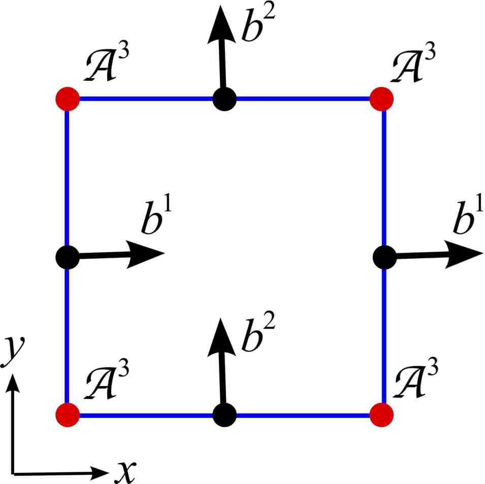
(b)

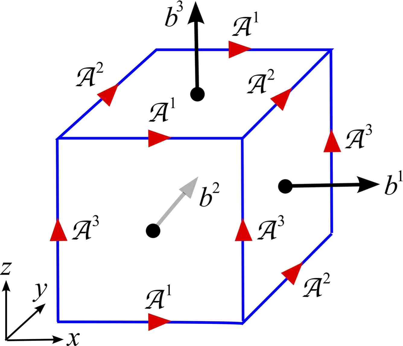
Fig. 1: Staggered magnetic field and magnetic potential configurations for Cartesian mesh elements. Shown in Panel (a) is a 2D mesh element with the magnetic field components on mesh edges and the potential on mesh corners. Shown in Panel (b) is a 3D mesh element with the magnetic field components on mesh faces and the potential on mesh edges.

5.2 2D construction of a divergence-free magnetic field

The final pieces missing from the constrained transport method as proposed in this work are the details of the divergence-free construction step as referred to in (99). The approach advocated here is a modification of similar divergence-free constructions used by Balsara [1] and Li, Xu, and Yakovlev [25]. In fact, the divergence-free reconstruction of the magnetic field is directly related to ideas from discrete exterior calculus and, in particular, to Whitney forms (e.g., see Bossavit [6]). Despite these connections, we do need the full machinery of discrete exterior calculus and Whitney forms in order to develop the proposed numerical scheme.

In 2D the divergence-free reconstruction makes use of magnetic field components normal to element edges and magnetic vector potential values on element corners. This grid staggering is illustrated in Figure 1(a). We give the full details of the divergence-free reconstruction below:

Step 0.

Start with the predicted magnetic field and the magnetic potential:

$$\widetilde{{\bf B}}^{h}\left({\bf x}\right)\cdot{\bf e}^{m}\Bigl{|}_{{\mathcal{T}}_{ij}}=\sum_{\ell=1}^{6}\widetilde{B}^{\,m(\ell)}_{ij}\,\varphi^{(\ell)}\left(\xi,\eta\right)\qquad\text{and}\qquad{\bf A}^{h}\left({\bf x}\right)\cdot{\bf e}^{3}\Bigl{|}_{{\mathcal{T}}_{ij}}=\sum_{\ell=1}^{6}A^{3(\ell)}_{ij}\,\varphi^{(\ell)}\left(\xi,\eta\right).$$ (101)

Step 1.

Interpolate the magnetic potential to mesh corners:

$${\mathcal{A}}^{3}_{i-\frac{1}{2}\,j-\frac{1}{2}}:=\frac{1}{4}\sum_{\ell=1}^{6}\biggl{[}A^{3(\ell)}_{ij}\,\varphi^{(\ell)}{\left(-1,-1\right)}+A^{3(\ell)}_{ij-1}\,\varphi^{(\ell)}\left(-1,1\right)+A^{3(\ell)}_{i-1j}\,\varphi^{(\ell)}\left(1,-1\right)+A^{3(\ell)}_{i-1j-1}\,\varphi^{(\ell)}\left(1,1\right)\biggr{]}.$$ (102)

Step 2.

On each element edge, define a DG representation for the normal components of the magnetic field:

$$b^{1}_{i-\frac{1}{2}\,j}=\sum_{\ell=1}^{3}b^{1(\ell)}_{i-\frac{1}{2}\,j}\,\varphi_{\text{1D}}^{(\ell)}\left(\alpha\right)\qquad\text{and}\qquad b^{2}_{i\,j-\frac{1}{2}}=\sum_{\ell=1}^{3}b^{2(\ell)}_{i\,j-\frac{1}{2}}\,\varphi_{\text{1D}}^{(\ell)}\left(\alpha\right),$$ (103)

where $\varphi_{\text{1D}}^{(\ell)}$ are the 1D Legendre polynomials. The coefficients of $b^{1}$ and $b^{2}$ are primarily computed from direct interpolation of element centered magnetic field values: $\widetilde{{\bf B}}^{h}$. The exceptions to this are the average magnetic values on the edges, which, in order to guarantee zero divergence, are computed from finite differences of the magnetic potential on element corners. The detailed equations can be written as follows:

$$b^{1(1)}_{i-\frac{1}{2}\,j} =\frac{{\mathcal{A}}^{3}_{\,i-\frac{1}{2}\,j+\frac{1}{2}}-{\mathcal{A}}^{3}_{\,i-\frac{1}{2}\,j-\frac{1}{2}}}{\Delta y}, b^{2(1)}_{i\,j-\frac{1}{2}} =\frac{{\mathcal{A}}^{3}_{\,i-\frac{1}{2}\,j-\frac{1}{2}}-{\mathcal{A}}^{3}_{\,i+\frac{1}{2}\,j-\frac{1}{2}}}{\Delta x},$$ (104)

$$b^{1(2)}_{i-\frac{1}{2}\,j} =\frac{\widetilde{B}^{\,1(3)}_{i-1j}+\sqrt{3}\,\widetilde{B}^{\,1(4)}_{i-1j}+\widetilde{B}^{\,1(3)}_{ij}-\sqrt{3}\,\widetilde{B}^{\,1(4)}_{ij}}{2}, b^{2(2)}_{i\,j-\frac{1}{2}} =\frac{\widetilde{B}^{\,2(2)}_{ij-1}+\sqrt{3}\,\widetilde{B}^{\,2(4)}_{ij-1}+\widetilde{B}^{2(2)}_{ij}-\sqrt{3}\,\widetilde{B}^{\,2(4)}_{ij}}{2},$$ (105)

$$b^{1(3)}_{i-\frac{1}{2}\,j} =\frac{\widetilde{B}^{\,1(6)}_{i-1j}+\widetilde{B}^{\,1(6)}_{ij}}{2}, b^{2(3)}_{i\,j-\frac{1}{2}} =\frac{\widetilde{B}^{\,2(5)}_{ij-1}+\widetilde{B}^{\,2(5)}_{ij}}{2}.$$ (106)

Step 3.

The final step is to construct globally divergence-free magnetic field values:

$${{\bf B}}^{h}\left({\bf x}\right)\cdot{\bf e}^{1}\Bigl{|}_{{\mathcal{T}}_{ij}}=\sum_{\ell=1}^{10}B^{\,1(\ell)}_{ij}\,\varphi^{(\ell)}\left(\xi,\eta\right)\qquad\text{and}\qquad{{\bf B}}^{h}\left({\bf x}\right)\cdot{\bf e}^{2}\Bigl{|}_{{\mathcal{T}}_{ij}}=\sum_{\ell=1}^{10}B^{\,2(\ell)}_{ij}\,\varphi^{(\ell)}\left(\xi,\eta\right).$$ (107)

This is achieved by enforcing the following conditions:

1. ${{\bf B}}^{h}\left({\bf x}\right)\cdot{\bf e}^{1}$ exactly matches $b^{1}$ from (103) on the left $(i-\frac{1}{2},j)$ and right $(i+\frac{1}{2},j)$ edges;

2. ${{\bf B}}^{h}\left({\bf x}\right)\cdot{\bf e}^{2}$ exactly matches $b^{2}$ from (103) on the bottom $(i,j-\frac{1}{2})$ and top $(i,j+\frac{1}{2})$ edges;

3. $\nabla\cdot{{\bf B}}^{h}\Bigl{|}_{{\mathcal{T}}_{ij}}=\text{constant}$; and

4. Any coefficients in (107) that remain as free parameters are set to zero.

The detailed equations for the 1-component can be written as follows:

$$\begin{split}B^{1(1)}_{ij}&=\frac{1}{2}\left(b_{i+\frac{1}{2}\,j}^{1\,(1)}+b_{i-\frac{1}{2}\,j}^{1\,(1)}\right)+\frac{1}{2\sqrt{3}}\frac{\Delta x}{\Delta y}\left(b_{i\,j+\frac{1}{2}}^{2\,(2)}-b_{i\,j-\frac{1}{2}}^{2\,(2)}\right),\\ B^{1(2)}_{ij}&=\frac{1}{2\sqrt{3}}\left(b_{i+\frac{1}{2}\,j}^{1\,(1)}-b_{i-\frac{1}{2}\,j}^{1\,(1)}\right)+\frac{1}{2\sqrt{15}}\frac{\Delta x}{\Delta y}\left(b_{i\,j+\frac{1}{2}}^{2\,(3)}-b_{i\,j-\frac{1}{2}}^{2\,(3)}\right),\\ B^{1(3)}_{ij}&=\frac{1}{2}\left(b_{i+\frac{1}{2}\,j}^{1\,(2)}+b_{i-\frac{1}{2}\,j}^{1\,(2)}\right),\quad B^{1(4)}_{ij}=\frac{1}{2\sqrt{3}}\left(b_{i+\frac{1}{2}\,j}^{1\,(2)}-b_{i-\frac{1}{2}\,j}^{1\,(2)}\right),\\ B^{1(5)}_{ij}&=\frac{1}{2\sqrt{15}}\frac{\Delta x}{\Delta y}\left(b_{i\,j-\frac{1}{2}}^{2\,(2)}-b_{i\,j+\frac{1}{2}}^{2\,(2)}\right),\quad B^{1(6)}_{ij}=\frac{1}{2}\left(b_{i+\frac{1}{2}\,j}^{1\,(3)}+b_{i-\frac{1}{2}\,j}^{1\,(3)}\right),\quad B^{1(7)}_{ij}=0,\\ B^{1(8)}_{ij}&=\frac{1}{2\sqrt{3}}\left(b_{i+\frac{1}{2}\,j}^{1\,(3)}-b_{i-\frac{1}{2}\,j}^{1\,(3)}\right),\quad B^{1(9)}_{ij}=\frac{1}{2\sqrt{35}}\frac{\Delta x}{\Delta y}\left(b_{i\,j-\frac{1}{2}}^{2\,(3)}-b_{i\,j+\frac{1}{2}}^{2\,(3)}\right),\quad B^{1(10)}_{ij}=0,\end{split}$$ (108)

The detailed equations for the 2-component can be written as follows:

$$\begin{split}B^{2(1)}_{ij}&=\frac{1}{2}\left(b_{i\,j+\frac{1}{2}}^{2\,(1)}+b_{i\,j-\frac{1}{2}}^{2\,(1)}\right)+\frac{1}{2\sqrt{3}}\frac{\Delta y}{\Delta x}\left(b_{i+\frac{1}{2}\,j}^{1\,(2)}-b_{i-\frac{1}{2}\,j}^{1\,(2)}\right),\quad B^{2(2)}_{ij}=\frac{1}{2}\left(b_{i\,j+\frac{1}{2}}^{2\,(2)}+b_{i\,j-\frac{1}{2}}^{2\,(2)}\right),\\ B^{2(3)}_{ij}&=\frac{1}{2\sqrt{3}}\left(b_{i\,j+\frac{1}{2}}^{2\,(1)}-b_{i\,j-\frac{1}{2}}^{2\,(1)}\right)+\frac{1}{2\sqrt{15}}\frac{\Delta y}{\Delta x}\left(b_{i+\frac{1}{2}\,j}^{1\,(3)}-b_{i-\frac{1}{2}\,j}^{1\,(3)}\right),\quad B^{2(4)}_{ij}=\frac{1}{2\sqrt{3}}\left(b_{i\,j+\frac{1}{2}}^{2\,(2)}-b_{i\,j-\frac{1}{2}}^{2\,(2)}\right),\\ B^{2(5)}_{ij}&=\frac{1}{2}\left(b_{i\,j+\frac{1}{2}}^{2\,(3)}+b_{i\,j-\frac{1}{2}}^{2\,(3)}\right),\quad B^{2(6)}_{ij}=\frac{1}{2\sqrt{15}}\frac{\Delta y}{\Delta x}\left(b_{i-\frac{1}{2}\,j}^{1\,(2)}-b_{i+\frac{1}{2}\,j}^{1\,(2)}\right),\\ B^{2(7)}_{ij}&=\frac{1}{2\sqrt{3}}\left(b_{i\,j+\frac{1}{2}}^{2\,(3)}-b_{i\,j-\frac{1}{2}}^{2\,(3)}\right),\quad B^{2(8)}_{ij}=B^{2(9)}_{ij}=0,\quad B^{2(10)}_{ij}=\frac{1}{2\sqrt{35}}\frac{\Delta y}{\Delta x}\left(b_{i-\frac{1}{2}\,j}^{1\,(3)}-b_{i+\frac{1}{2}\,j}^{1\,(3)}\right).\end{split}$$ (109)

A straightforward calculation reveals that the (pointwise) divergence of a magnetic field of the form (107) with coefficients given by (108) and (109) is

$$\nabla\cdot{\bf B}^{h}\Bigl{|}_{{\mathcal{T}}_{ij}}=\frac{2}{\Delta x}\frac{\partial}{\partial\xi}\left({{\bf B}}^{h}\left({\bf x}\right)\cdot{\bf e}^{1}\Bigl{|}_{{\mathcal{T}}_{ij}}\right)+\frac{2}{\Delta y}\frac{\partial}{\partial\eta}\left({{\bf B}}^{h}\left({\bf x}\right)\cdot{\bf e}^{2}\Bigl{|}_{{\mathcal{T}}_{ij}}\right)=\frac{b_{i+\frac{1}{2}\,j}^{1\,(1)}-b_{i-\frac{1}{2}\,j}^{1\,(1)}}{\Delta x}+\frac{b_{i\,j+\frac{1}{2}}^{2\,(1)}-b_{i\,j-\frac{1}{2}}^{2\,(1)}}{\Delta y},$$ (110)

which is constant. Using definitions (104), this divergence can be shown to vanish:

$$\nabla\cdot{\bf B}^{h}\Bigl{|}_{{\mathcal{T}}_{ij}}=\frac{{\mathcal{A}}^{3}_{\,i+\frac{1}{2}\,j+\frac{1}{2}}-{\mathcal{A}}^{3}_{\,i+\frac{1}{2}\,j-\frac{1}{2}}-{\mathcal{A}}^{3}_{\,i-\frac{1}{2}\,j+\frac{1}{2}}+{\mathcal{A}}^{3}_{\,i-\frac{1}{2}\,j-\frac{1}{2}}+{\mathcal{A}}^{3}_{\,i-\frac{1}{2}\,j+\frac{1}{2}}-{\mathcal{A}}^{3}_{\,i+\frac{1}{2}\,j+\frac{1}{2}}-{\mathcal{A}}^{3}_{\,i-\frac{1}{2}\,j-\frac{1}{2}}+{\mathcal{A}}^{3}_{\,i+\frac{1}{2}\,j-\frac{1}{2}}}{\Delta x\,\Delta y}=0.$$

We note that we have actually achieved a globally divergence free magnetic field, ${\bf B}^{h}({\bf x})$, since we have the two sufficient ingredients:

1. ${\bf B}^{h}({\bf x})$ restricted to the interior of each element is exactly divergence-free (see (110)); and

2. The normal components of ${\bf B}^{h}({\bf x})$ are continuous across each element edge (see (108)–(109)).

5.3 3D construction of a divergence-free magnetic field

The same basic principle used in 2D can be extended to construct a globally divergence-free magnetic field in 3D. In 3D the divergence-free reconstruction makes use of magnetic field components normal to element faces and magnetic vector potential values on element edges. This grid staggering is illustrated in Figure 1(b). We outline the divergence-free reconstruction procedure below:

Step 0.

Start with the predicted magnetic field and magnetic potential:

$$\widetilde{{\bf B}}^{h}\left({\bf x}\right)\cdot{\bf e}^{m}\Bigl{|}_{{\mathcal{T}}_{ijk}}=\sum_{\ell=1}^{10}\widetilde{B}^{\,m(\ell)}_{ijk}\,\varphi^{(\ell)}\left(\xi,\eta,\zeta\right)\qquad\text{and}\qquad{\bf A}^{h}\left({\bf x}\right)\cdot{\bf e}^{m}\Bigl{|}_{{\mathcal{T}}_{ijk}}=\sum_{\ell=1}^{10}A^{m(\ell)}_{ijk}\,\varphi^{(\ell)}\left(\xi,\eta,\zeta\right).$$ (111)

Step 1.

Interpolate the magnetic potential to mesh edges:

$$\begin{split}{\mathcal{A}}^{1}_{i\,j-\frac{1}{2}\,k-\frac{1}{2}}:=\frac{1}{8}\sum_{\ell=1}^{10}\int_{-1}^{1}\biggl{[}&A^{1(\ell)}_{ijk}\,\varphi^{(\ell)}\left(\xi,-1,-1\right)+A^{1(\ell)}_{ijk-1}\,\varphi^{(\ell)}\left(\xi,-1,1\right)\\ +\,\,&A^{1(\ell)}_{ij-1k}\,\varphi^{(\ell)}\left(\xi,1,-1\right)+A^{1(\ell)}_{ij-1k-1}\,\varphi^{(\ell)}\left(\xi,1,1\right)\biggr{]}\,d\xi,\end{split}$$ (112)

$$\begin{split}{\mathcal{A}}^{2}_{i-\frac{1}{2}\,j\,k-\frac{1}{2}}:=\frac{1}{8}\sum_{\ell=1}^{10}\int_{-1}^{1}\biggl{[}&A^{2(\ell)}_{ijk}\,\varphi^{(\ell)}\left(-1,\eta,-1\right)+A^{2(\ell)}_{ijk-1}\,\varphi^{(\ell)}\left(-1,\eta,1\right)\\ +\,\,&A^{2(\ell)}_{i-1jk}\,\varphi^{(\ell)}\left(1,\eta,-1\right)+A^{2(\ell)}_{i-1jk-1}\,\varphi^{(\ell)}\left(1,\eta,1\right)\biggr{]}\,d\eta,\end{split}$$ (113)

$$\begin{split}{\mathcal{A}}^{3}_{i-\frac{1}{2}\,j-\frac{1}{2}\,k}:=\frac{1}{8}\sum_{\ell=1}^{10}\int_{-1}^{1}\biggl{[}&A^{3(\ell)}_{ijk}\,\varphi^{(\ell)}\left(-1,-1,\zeta\right)+A^{3(\ell)}_{ij-1k}\,\varphi^{(\ell)}\left(-1,1,\zeta\right)\\ +\,\,&A^{3(\ell)}_{i-1jk}\,\varphi^{(\ell)}\left(1,-1,\zeta\right)+A^{3(\ell)}_{i-1j-1k}\,\varphi^{(\ell)}\left(1,1,\zeta\right)\biggr{]}\,d\zeta.\end{split}$$ (114)

Note that these magnetic potential values are the edge averages of the magnetic potential; for example, ${\mathcal{A}}^{1}_{i\,j-\frac{1}{2}\,k-\frac{1}{2}}$ is an approximation to the average of $A^{1}(x,y_{j}-\Delta y/2,z_{k}-\Delta z/2)$ over the interval $x\in[x_{i}-\Delta x/2,x_{i}+\Delta x/2]$.

Step 2.

On each element face, define a DG representation for the normal components of the magnetic field:

$$\left\{b^{1}_{i-\frac{1}{2}\,j\,k},\,b^{2}_{i\,j-\frac{1}{2}\,k},\,b^{3}_{i\,j\,k-\frac{1}{2}}\right\} =\sum_{\ell=1}^{6}\left\{b^{1(\ell)}_{i-\frac{1}{2}\,j\,k},\,b^{2(\ell)}_{i\,j-\frac{1}{2}\,k},\,b^{3(\ell)}_{i\,j\,k-\frac{1}{2}}\right\}\,\varphi_{\text{2D}}^{(\ell)}\left(\alpha,\,\beta\right),$$ (115)

where $\varphi_{\text{2D}}^{(\ell)}$ are the 2D Legendre polynomials (35). The coefficients of $b^{1}$, $b^{2}$, and $b^{3}$ are primarily computed from direct interpolation of element centered magnetic field values, $\widetilde{{\bf B}}^{h}$. The exceptions to this are the average magnetic values on the faces, which, in order to guarantee zero divergence, are computed from finite differences of the average magnetic potential on element edges. The full formulas are given by (129)-(131).

Step 3.

The final step is to construct globally divergence-free magnetic field values:

$${{\bf B}}^{h}\left({\bf x}\right)\cdot{\bf e}^{m}\Bigl{|}_{{\mathcal{T}}_{ijk}}=\sum_{\ell=1}^{20}B^{\,m(\ell)}_{ijk}\,\varphi^{(\ell)}\left(\xi,\eta,\zeta\right).$$ (116)

This is achieved by enforcing the following conditions:

1. ${{\bf B}}^{h}\left({\bf x}\right)\cdot{\bf e}^{1}$ exactly matches $b^{1}$ from (115) on the left $(i-\frac{1}{2},j,k)$ and right $(i+\frac{1}{2},j,k)$ faces;

2. ${{\bf B}}^{h}\left({\bf x}\right)\cdot{\bf e}^{2}$ exactly matches $b^{2}$ from (115) on the front $(i,j-\frac{1}{2},k)$ and back $(i,j+\frac{1}{2},k)$ faces;

3. ${{\bf B}}^{h}\left({\bf x}\right)\cdot{\bf e}^{3}$ exactly matches $b^{3}$ from (115) on the bottom $(i,j,k-\frac{1}{2})$ and top $(i,j,k+\frac{1}{2})$ faces;

4. $\nabla\cdot{{\bf B}}^{h}\Bigl{|}_{{\mathcal{T}}_{ijk}}=\text{constant}$; and

5. Any coefficients in (116) that remain as free parameters are set to zero.

The full formulas are given by (132)–(154).

A straightforward calculation reveals that the (pointwise) divergence of a magnetic field of the form (116) with coefficients given by (132)–(164) is

$$\nabla\cdot{\bf B}^{h}\Bigl{|}_{{\mathcal{T}}_{ijk}}=\frac{b^{1}_{i+\frac{1}{2}jk}-b^{1}_{i-\frac{1}{2}jk}}{\Delta x}+\frac{b^{2}_{ij+\frac{1}{2}k}-b^{2}_{ij-\frac{1}{2}k}}{\Delta y}+\frac{b^{3}_{ijk+\frac{1}{2}}-b^{3}_{ijk-\frac{1}{2}}}{\Delta z},$$ (117)

which is constant. Using definitions (129), (130), and (131), this divergence can be shown to vanish:

$$\nabla\cdot{\bf B}^{h}\Bigl{|}_{{\mathcal{T}}_{ijk}}=0.$$ (118)

Just as in the 2D case, we note that we have actually achieved a globally divergence free magnetic field, ${\bf B}^{h}({\bf x})$.

6 Numerical examples

In this section we apply the proposed 2D and 3D constrained transport schemes to four numerical test cases. For both the 2D and 3D versions, we consider first a smooth problem to verify the order of accuracy of the proposed scheme, followed by a problem with shock waves to verify the shock-capturing ability of the scheme. All four examples considered in this work make use of double (2D) or triple (3D) periodic boundary conditions on the conservative variables: $\rho$, $\rho{\bf u}$, ${\mathcal{E}}$, and ${\bf B}$. In our constrained transport scheme, no explicit boundary conditions are needed for ${\bf A}$, since ${\bf A}$ is updated via (93) using velocity and magnetic fields that satisfy the appropriate boundary conditions.

6.1 2D smooth Alfvén wave problem

We consider a smooth circular polarized Alfvén wave that propagates in direction ${\bf n}=[\cos\phi,\sin\phi,0]^{T}$ towards the origin. This problem has been considered by several authors (e.g., [20, 32, 36]). The problem consists of smooth initial data on $\left[0,{1}/{\cos\phi}\right]\times\left[0,{1}/{\sin\phi}\right]$, where $\phi=\tan^{-1}(0.5)$:

$$\rho=1,\quad{\bf u}=\left[-u^{t}\sin\phi,\,\,u^{t}\cos\phi,\,\,u^{r}\right]^{T},\quad p=0.1,\quad{\bf B}=\left[\cos\phi-u^{t}\sin\phi,\,\,\sin\phi+u^{t}\cos\phi,\,\,u^{r}\right]^{T},$$ (119)

where

$$u^{t}=0.1\sin\left(2\pi\left(x\cos\phi+y\sin\phi\right)\right)\quad\text{and}\quad u^{r}=0.1\cos\left(2\pi\left(x\cos\phi+y\sin\phi\right)\right).$$ (120)

This example is used to verify the order of accuracy of the proposed 2D constrained transport scheme.

Experimental convergence rates are shown in Table 1. The errors are calculated by computing the $L^{2}$-difference between the computed solution in ${\mathcal{W}}^{h}_{2}$ and the exact solution projected into ${\mathcal{W}}^{h}_{3}$:

$$\frac{\|q^{\text{exact}}-q^{h}\|_{L^{2}}}{\|q^{\text{exact}}\|_{L^{2}}}\approx\left[{{\sum_{ij}\left(\sum_{\ell=1}^{6}\left\{Q^{\text{exact}\,(\ell)}_{ij}-Q^{(\ell)}_{ij}\right\}+\sum_{\ell=7}^{10}Q^{\text{exact}\,(\ell)}_{ij}\right)}}\right]^{\frac{1}{2}}\cdot\left[{{\sum_{ij}\left(\sum_{\ell=1}^{10}Q^{\text{exact}\,(\ell)}_{ij}\right)}}\right]^{-\frac{1}{2}}.$$ (121)

In particular, in Table 1 we show the computed relative $L^{2}$-errors at time $t=2$ (i.e., after 2 periods of the Alfvén wave). Experimental convergence rates are calculated using a least squares fit through the computed errors. This table clearly shows the third order convergence of the proposed numerical scheme. Furthermore, in Figure 2, we show on a mesh with $16\times 32$ elements and at time $t=2$ scatter plots of the computed (a) magnetic field perpendicular to the direction of propagation ($B^{\perp}$) and (b) periodic part of the magnetic potential ($A^{3}-\left(y\cos\phi-x\sin\phi\right)$). These plots show that the computed solution is in very good agreement with the exact solution.

6.2 2D Orszag-Tang vortex problem

Next we consider the Orszag-Tang vortex problem, which is widely considered a standard test example for MHD in the literature (see Tóth [36]). The problem consists of smooth initial data on $[0,2\pi]\times[0,2\pi]$:

$$\rho=\gamma^{2},\quad{\bf u}=\Bigl{[}-\sin y,\,\sin x,\,0\Bigr{]}^{T},\quad p=\gamma,\quad{\bf B}=\Bigl{[}-\sin y,\,\sin(2x),\,0\Bigr{]}^{T},\quad A^{3}=\frac{1}{2}\cos(2x)+\cos y.$$ (122)

In this problem, the variable magnetic field eventually causes the smooth initial data to form a strong rotating shock structure. It has been well documented in the literature (e.g., see Tóth [36], Rossmanith [32], and Li and Shu [24]) that the formation of this shock structure can lead to numerical instabilities in numerical methods that do not control magnetic field divergence errors.

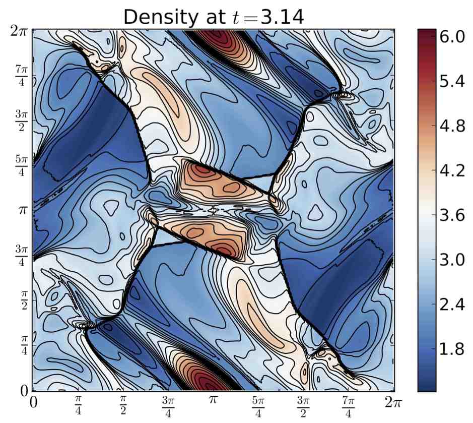
(a)	(b)
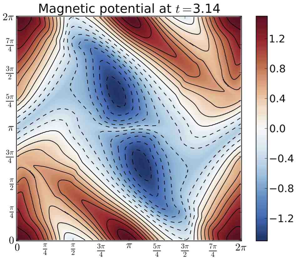
(c)	(d)

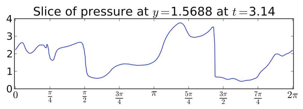
Fig. 3: Orszag-Tang vortex problem in 2D run on a mesh with $257\times 257$ mesh elements. Shown in these panels are the (a) mass density: $\rho(t,{\bf x})$, (b) magnetic potential: $A^{3}(t,{\bf x})$, (c) pressure: $p(t,{\bf x})$, and (d) a slice of the pressure at $y=1.5688$, all at the final time in the solution: $t=3.14$.

The solution with the proposed scheme is shown in Figure 3. In particular, we show at time $t=3.14$ on a mesh with $257\times 257$ elements the (a) mass density: $\rho(t,{\bf x})$, (b) magnetic potential: $A^{3}(t,{\bf x})$, (c) pressure: $p(t,{\bf x})$, and (d) a slice of the pressure at $y=1.5688$. These results are in good agreement with the published literature, and clearly demonstrate the ability of the proposed numerical scheme to remain stable for a problem with complicated shock structures.

6.3 3D smooth Alfvén wave problem

In order to verify the order of convergence of the 3D constrained transport method we consider a 3D version of the smooth Alfvén wave problem considered in Helzel et al. [20]. In this case the wave propagates in the direction ${\bf n}=\left[\cos\phi\cos\theta,\,\sin\phi\cos\theta,\,\sin\theta\right]^{T}$ towards the origin. Here $\phi$ is an angle with respect to the $x$-axis in the $xy$-plane and $\theta$ is an angle with respect to the $x$-axis in the $xz$-plane. We take $\theta=\phi=\tan^{-1}(0.5)\approx 26.5651^{\circ}$. The problem consists of smooth initial data on $\left[0,\left({\cos\phi\cos\theta}\right)^{-1}\right]\times\left[0,\left({\sin\phi\cos\theta}\right)^{-1}\right]\times\left[0,\left({\sin\theta}\right)^{-1}\right]$:

$$\rho=\gamma^{2},\quad{\bf u}=u^{t}\,{\bf t}+u^{r}\,{\bf r},\quad p=\gamma,\quad{\bf B}={\bf n}+B^{t}\,{\bf t}+B^{r}\,{\bf r},$$ (123)

where

$$u^{t}=0.1\sin\left(2\pi\,{\bf x}\cdot{\bf n}\right),\quad u^{r}=0.1\cos\left(2\pi\,{\bf x}\cdot{\bf n}\right),$$ (124)

and ${\bf t}=\left[-\sin\phi,\cos\phi,0\right]^{T}$ and ${\bf r}=\left[-\cos\phi\sin\theta,-\sin\phi\sin\theta,\cos\theta\right]^{T}$. The initial magnetic vector potential is

$${\bf A} =\left[z\sin\phi\cos\theta-\frac{\sin\phi\sin(2\pi\,{\bf n}\cdot{\bf x})}{20\pi},\,\,\,x\sin\theta+\frac{\cos\phi\sin(2\pi\,{\bf n}\cdot{\bf x})}{20\pi},\,\,\,y\cos\phi\cos\theta+\frac{\cos(2\pi\,{\bf n}\cdot{\bf x})}{20\pi\cos\theta}\right]^{T}.$$ (125)

Experimental convergence rates are shown in Table 2. The errors are calculated by computing the $L^{2}$-difference between the computed solution in ${\mathcal{W}}^{h}_{2}$ and the exact solution projected into ${\mathcal{W}}^{h}_{3}$:

$$\frac{\|q^{\text{exact}}-q^{h}\|_{L^{2}}}{\|q^{\text{exact}}\|_{L^{2}}}\approx\left[{{\sum_{ijk}\left(\sum_{\ell=1}^{10}\left\{Q^{\text{exact}\,(\ell)}_{ijk}-Q^{(\ell)}_{ijk}\right\}^{2}+\sum_{\ell=11}^{20}\left\{Q^{\text{exact}\,(\ell)}_{ijk}\right\}^{2}\right)}}\right]^{\frac{1}{2}}\cdot\left[{{\sum_{ijk}\sum_{\ell=1}^{20}\left\{Q^{\text{exact}\,(\ell)}_{ijk}\right\}^{2}}}\right]^{-\frac{1}{2}}.$$ (126)

In particular, in Table 2 we show the computed relative $L^{2}$-errors at time $t=2$ (i.e., after 2 periods of the Alfvén wave). Experimental convergence rates are calculated using a least squares fit through the computed errors. This table clearly shows the third order convergence of the proposed numerical scheme in all of the magnetic field and magnetic vector potential components.

6.4 3D Orszag-Tang vortex problem

Finally, we consider a 3D version of the Orszag-Tang vortex problem as considered in Helzel et al. [20]. The problem consists of smooth initial data on $[0,2\pi]\times[0,2\pi]\times[0,2\pi]$:

$$\rho=\gamma^{2},\quad{\bf u}=\Bigl{[}-(1+\varepsilon\sin z)\sin y,\,\,(1+\varepsilon\sin z)\sin x,\,\,\varepsilon\sin z\Bigr{]}^{T},\quad p=\gamma,\quad{\bf B}=\Bigl{[}-\sin y,\,\,\sin(2x),\,\,0\Bigr{]}^{T},$$ (127)

where $\varepsilon=0.2$. The initial condition for the magnetic potential is

$${\bf A}=\Bigl{[}0,\,\,0,\,\,\frac{1}{2}\cos(2x)+\cos y\Bigr{]}^{T}.$$ (128)

Just as in the 2D problem, the variable magnetic field eventually causes the smooth initial data to form a strong rotating shock structure. The formation of this shock structure can lead to numerical instabilities in numerical methods that do not control magnetic field divergence errors.

We computed a solution on a mesh with $129\times 129\times 129$ elements out to time $t=3$. The results are shown at different horizontal slices in Figures 4 ($z\approx 1.53$), 5 ($z\approx 4.75$), and 6 ($z\approx 3.14$). In particular, in each of these plots we show the (a) mass density: $\rho(t,{\bf x})$, (b) pressure: $p(t,{\bf x})$, and (c) $z$-component of the magnetic potential: $A^{3}(t,{\bf x})$. These results are in good agreement with those presented in Helzel et al. [20], and clearly demonstrate the ability of the proposed numerical scheme to remain stable for a problem with complicated shock structures.

Mesh	Rel. $L^{2}$ error in $B^{1}$	Rel. $L^{2}$ error in $B^{2}$	Rel. $L^{2}$ error in $A^{3}$
$8\times 16$	$8.8697\times 10^{-4}$	$3.4907\times 10^{-3}$	$3.3831\times 10^{-4}$
$16\times 32$	$1.0344\times 10^{-4}$	$4.0578\times 10^{-4}$	$3.8084\times 10^{-5}$
$32\times 64$	$1.3349\times 10^{-5}$	$5.2515\times 10^{-5}$	$4.6941\times 10^{-6}$
$64\times 128$	$1.7216\times 10^{-6}$	$6.798\times 10^{-6}$	$5.9009\times 10^{-7}$
$128\times 256$	$2.1876\times 10^{-7}$	$8.6605\times 10^{-7}$	$7.4004\times 10^{-8}$
Least squares order	2.9879	2.9853	3.0329

Table 1: Relative $L^{2}$ errors in $B^{1}$, $B^{2}$, and $A^{3}$ for several mesh resolutions on the 2D smooth Alfvén wave problem. For each component we use a least squares fit to estimate the order of accuracy.

(a)

(b)

Fig. 2: Scatter plots of the constrained transport DG-FEM solution for the 2D smooth Alfvén wave on a $16\times 32$ Cartesian mesh. Panel (a) shows the magnetic field perpendicular to the direction of propagation, $B^{\perp}=B^{2}\cos\phi-B^{1}\sin\phi$, where $\phi=\tan^{-1}(0.5)$, as a function of the coordinate along the direction of propagation $\xi=x\cos\phi+y\sin\phi$. Panel (b) shows the periodic part of the magnetic potential, $A^{3}-\eta$, where $\eta=y\cos\phi-x\sin\phi$.

Mesh	Rel. $L^{2}$ error in $B^{1}$	Rel. $L^{2}$ error in $B^{2}$	Rel. $L^{2}$ error in $B^{3}$
$8\times 16\times 16$	$1.2159\times 10^{-3}$	$6.7737\times 10^{-3}$	$3.3457\times 10^{-3}$
$16\times 32\times 32$	$1.0804\times 10^{-4}$	$8.788\times 10^{-4}$	$4.9195\times 10^{-4}$
$32\times 64\times 64$	$1.1507\times 10^{-5}$	$1.124\times 10^{-4}$	$7.6376\times 10^{-5}$
$64\times 128\times 128$	$1.5083\times 10^{-6}$	$1.4831\times 10^{-5}$	$1.0894\times 10^{-5}$
Least squares order	3.2196	2.9472	2.7475

Mesh	Rel. $L^{2}$ error in $A^{1}$	Rel. $L^{2}$ error in $A^{2}$	Rel. $L^{2}$ error in $A^{3}$
$8\times 16\times 16$	$5.7994\times 10^{-4}$	$7.36\times 10^{-4}$	$3.5364\times 10^{-4}$
$16\times 32\times 32$	$8.0689\times 10^{-5}$	$9.2977\times 10^{-5}$	$4.4725\times 10^{-5}$
$32\times 64\times 64$	$1.0885\times 10^{-5}$	$1.5308\times 10^{-5}$	$5.6484\times 10^{-6}$
$64\times 128\times 128$	$1.4532\times 10^{-6}$	$2.2029\times 10^{-6}$	$7.2656\times 10^{-7}$
Least squares order	2.8812	2.7755	2.9766

Table 2: Relative $L^{2}$ errors in $B^{1}$, $B^{2}$, $B^{3}$, $A^{1}$, $A^{2}$, and $A^{3}$ for several mesh resolutions on the 3D smooth Alfvén wave problem. For each component we use a least squares fit to estimate the order of accuracy.

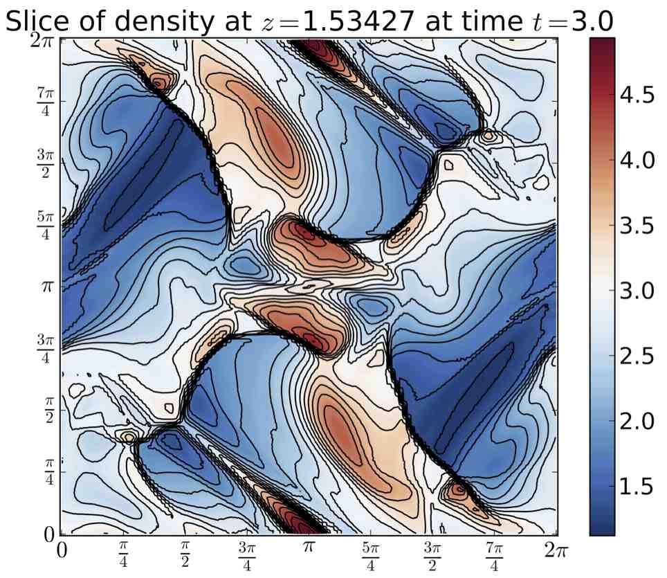
(a)	(b)
(c)

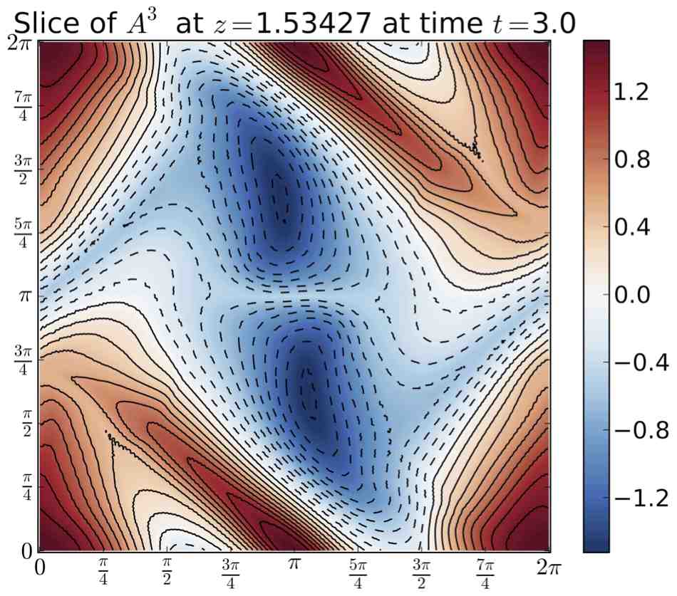
Fig. 4: Horizontal slice at $z=z_{32}\approx 1.534266180$ of the 3D Orszag-Tang vortex problem run on a mesh with $129\times 129\times 129$ mesh elements. Shown in these panels are the (a) mass density: $\rho(t,{\bf x})$, (b) pressure: $p(t,{\bf x})$, and (c) $z$-component of the magnetic potential: $A^{3}(t,{\bf x})$, all at time $t=3$.

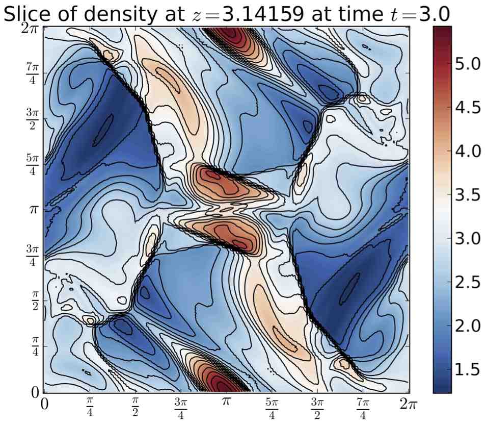
(a)	(b)
(c)

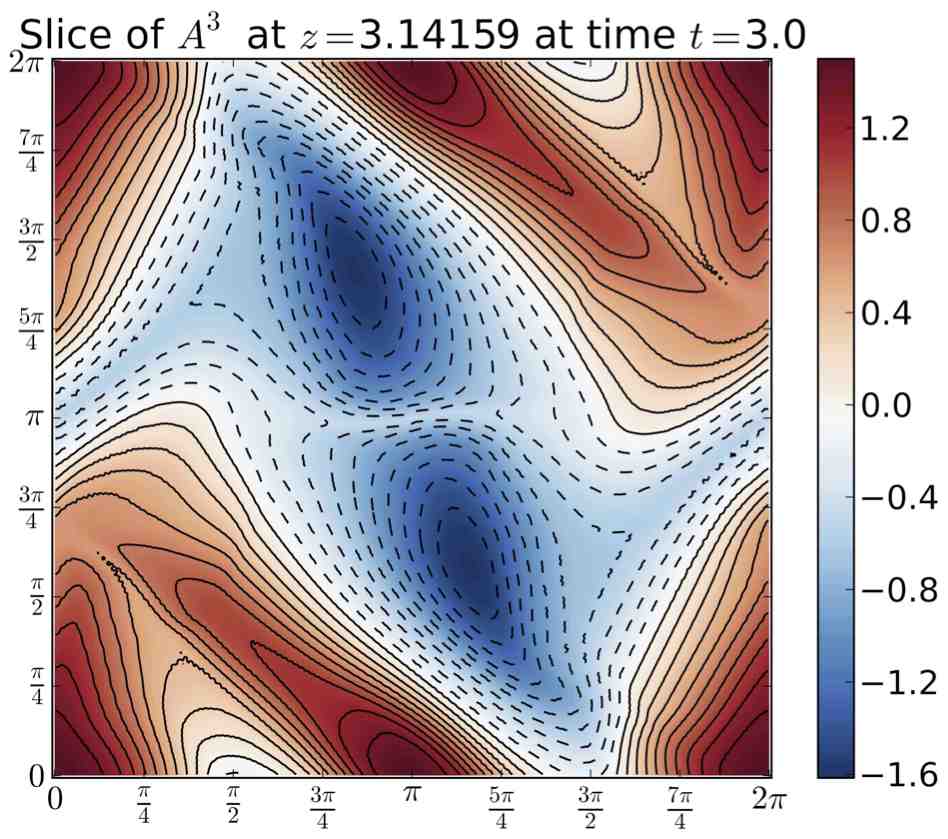
Fig. 5: Horizontal slice at $z=z_{65}\approx 3.141592654$ of the 3D Orszag-Tang vortex problem run on a mesh with $129\times 129\times 129$ mesh elements. Shown in these panels are the (a) mass density: $\rho(t,{\bf x})$, (b) pressure: $p(t,{\bf x})$, and (c) $z$-component of the magnetic potential: $A^{3}(t,{\bf x})$, all at time $t=3$.

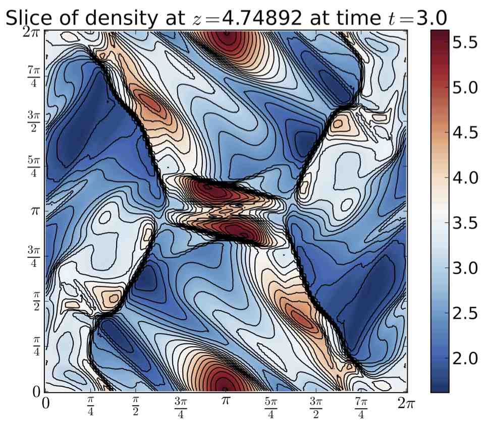
(a)	(b)
(c)

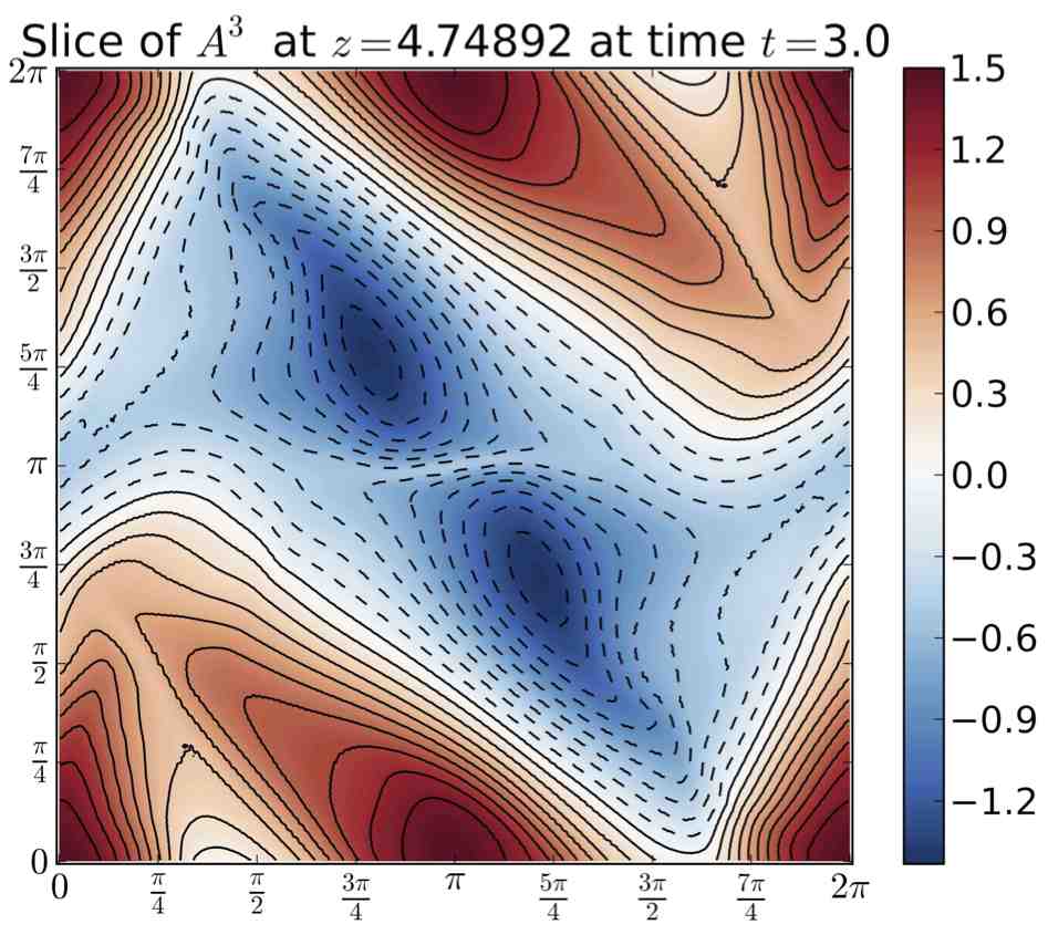
Fig. 6: Horizontal slice at $z=z_{98}\approx 4.748919128$ of the 3D Orszag-Tang vortex problem run on a mesh with $129\times 129\times 129$ mesh elements. Shown in these panels are the (a) mass density: $\rho(t,{\bf x})$, (b) pressure: $p(t,{\bf x})$, and (c) $z$-component of the magnetic potential: $A^{3}(t,{\bf x})$, all at time $t=3$.

7 Conclusions

In this work we showed how to extend the constrained transport framework originally proposed by Evans and Hawley [12] in the context of the discontinuous Galerkin finite element method (DG-FEM) on both 2D and 3D Cartesian meshes. The method presented in this work makes use of two key ingredients: (1) the introduction of a magnetic vector potential, which is represented in the same finite element space as the conserved variables, and (2) the use of a particular divergence-free reconstruction of the magnetic field, which makes use of the magnetic vector potential and the predicted magnetic field. The divergence-free reconstruction presented in this work is slight modification of the reconstruction method that has been used in other work on ideal MHD. Li, Xu, and Yakovlev [25] made use of this reconstruction in the context of a 2D central DG scheme. Balsara [1] made use this reconstruction in the context of finite volume schemes and adaptive mesh refinement. The novel aspect of this work is that we make direct use of a magnetic vector potential, thus following in the footsteps of the methods developed in [8, 20, 21, 26, 32, 35]. An advantage of our approach is that the extension from 2D to 3D is straightforward. The proposed scheme was then implemented in 2D and 3D using the DoGPack software package and applied on some standard MHD test cases. The results indicate that the proposed scheme is high-order accurate for smooth problems and is shock-capturing for problems with complicated multi-dimensional shock structures.

Acknowledgements. This work was supported in part by NSF grant DMS–1016202.

Appendix A 3D formulas for the construction of a divergence-free magnetic field

For completeness we include the formulas for computing the 3D divergence-free reconstruction of the magnetic field in this section. Refer to Figure 1(b) for the positioning of the various magnetic field and magnetic vector potential components. The magnetic field on left and right faces are defined as follows:

$$\begin{split}b^{1(1)}_{i-\frac{1}{2}\,j\,k}&=\frac{1}{\Delta y}\left({{\mathcal{A}}^{3}_{\,i-\frac{1}{2}\,j+\frac{1}{2}\,k}-{\mathcal{A}}^{3}_{\,i-\frac{1}{2}\,j-\frac{1}{2}\,k}}\right)-\frac{1}{\Delta z}\left({\mathcal{A}}^{2}_{\,i-\frac{1}{2}\,j\,k+\frac{1}{2}}-{\mathcal{A}}^{2}_{\,i-\frac{1}{2}\,j\,k-\frac{1}{2}}\right),\\ b^{1(2)}_{i-\frac{1}{2}\,j\,k}&=\frac{1}{2}\left(\widetilde{B}^{\,1(3)}_{i-1jk}+\sqrt{3}\widetilde{B}^{1(5)}_{i-1jk}+\widetilde{B}^{\,1(3)}_{ijk}-\sqrt{3}\widetilde{B}^{\,1(5)}_{ijk}\right),\quad b^{1(3)}_{i-\frac{1}{2}\,j\,k}=\frac{1}{2}\left(\widetilde{B}^{\,1(4)}_{i-1jk}+\sqrt{3}\widetilde{B}^{1(6)}_{i-1jk}+\widetilde{B}^{\,1(4)}_{ijk}-\sqrt{3}\widetilde{B}^{\,1(6)}_{ijk}\right),\\ b^{1(4)}_{i-\frac{1}{2}\,j\,k}&=\frac{1}{2}\left(\widetilde{B}^{\,1(7)}_{i-1jk}+\widetilde{B}^{\,1(7)}_{ijk}\right),\quad b^{1(5)}_{i-\frac{1}{2}\,j\,k}=\frac{1}{2}\left(\widetilde{B}^{\,1(9)}_{i-1jk}+\widetilde{B}^{\,1(9)}_{ijk}\right),\quad b^{1(6)}_{i-\frac{1}{2}\,j\,k}=\frac{1}{2}\left(\widetilde{B}^{\,1(10)}_{i-1jk}+\widetilde{B}^{\,1(10)}_{ijk}\right).\end{split}$$ (129)

The magnetic field on front and back faces are defined as follows:

$$\begin{split}b^{2(1)}_{i\,j-\frac{1}{2}\,k}&=\frac{1}{\Delta z}\left({\mathcal{A}}^{1}_{\,i\,j-\frac{1}{2}\,k+\frac{1}{2}}-{\mathcal{A}}^{1}_{\,i\,j-\frac{1}{2}\,k-\frac{1}{2}}\right)-\frac{1}{\Delta x}\left({\mathcal{A}}^{3}_{\,i+\frac{1}{2}\,j-\frac{1}{2}\,k}-{\mathcal{A}}^{3}_{\,i-\frac{1}{2}\,j-\frac{1}{2}\,k}\right),\\ b^{2(2)}_{i\,j-\frac{1}{2}\,k}&=\frac{1}{2}\left(\widetilde{B}^{\,2(2)}_{ij-1k}+\sqrt{3}\widetilde{B}^{\,2(5)}_{ij-1k}+\widetilde{B}^{\,2(2)}_{ijk}-\sqrt{3}\widetilde{B}^{\,2(5)}_{ijk}\right),\quad b^{2(3)}_{i\,j-\frac{1}{2}\,k}=\frac{1}{2}\left(\widetilde{B}^{\,2(4)}_{ij-1k}+\sqrt{3}\widetilde{B}^{\,2(7)}_{ij-1k}+\widetilde{B}^{\,2(4)}_{ijk}-\sqrt{3}\widetilde{B}^{\,2(7)}_{ijk}\right),\\ b^{2(4)}_{i\,j-\frac{1}{2}\,k}&=\frac{1}{2}\left(\widetilde{B}^{\,2(6)}_{ij-1k}+\widetilde{B}^{\,2(6)}_{ijk}\right),\quad b^{2(5)}_{i\,j-\frac{1}{2}\,k}=\frac{1}{2}\left(\widetilde{B}^{\,2(8)}_{ij-1k}+\widetilde{B}^{\,2(8)}_{ijk}\right),\quad b^{2(6)}_{i\,j-\frac{1}{2}\,k}=\frac{1}{2}\left(\widetilde{B}^{\,2(10)}_{ij-1k}+\widetilde{B}^{\,2(10)}_{ijk}\right).\end{split}$$ (130)

The magnetic field on bottom and top faces are defined as follows:

$$\begin{split}b^{3(1)}_{i\,j\,k-\frac{1}{2}}&=\frac{1}{\Delta x}\left({\mathcal{A}}^{2}_{\,i+\frac{1}{2}\,j\,k-\frac{1}{2}}-{\mathcal{A}}^{2}_{\,i-\frac{1}{2}\,j\,k-\frac{1}{2}}\right)-\frac{1}{\Delta y}\left({\mathcal{A}}^{1}_{\,i\,j+\frac{1}{2}\,k-\frac{1}{2}}-{\mathcal{A}}^{1}_{\,i\,j-\frac{1}{2}\,k-\frac{1}{2}}\right),\\ b^{3(2)}_{i\,j\,k-\frac{1}{2}}&=\frac{1}{2}\left(\widetilde{B}^{\,3(2)}_{ijk-1}+\sqrt{3}\widetilde{B}^{\,3(6)}_{ijk-1}+\widetilde{B}^{\,3(2)}_{ijk}-\sqrt{3}\widetilde{B}^{\,3(6)}_{ijk}\right),\quad b^{3(3)}_{i\,j\,k-\frac{1}{2}}=\frac{1}{2}\left(\widetilde{B}^{\,3(3)}_{ijk-1}+\sqrt{3}\widetilde{B}^{\,3(7)}_{ijk-1}+\widetilde{B}^{\,3(3)}_{ijk}-\sqrt{3}\widetilde{B}^{\,3(7)}_{ijk}\right),\\ b^{3(4)}_{i\,j\,k-\frac{1}{2}}&=\frac{1}{2}\left(\widetilde{B}^{\,3(5)}_{ijk-1}+\widetilde{B}^{\,3(5)}_{ijk}\right),\quad b^{3(5)}_{i\,j\,k-\frac{1}{2}}=\frac{1}{2}\left(\widetilde{B}^{\,3(8)}_{ijk-1}+\widetilde{B}^{\,3(8)}_{ijk}\right),\quad b^{3(6)}_{i\,j\,k-\frac{1}{2}}=\frac{1}{2}\left(\widetilde{B}^{\,3(9)}_{ijk-1}+\widetilde{B}^{\,3(9)}_{ijk}\right).\end{split}$$ (131)

From these normal components on faces, we can reconstruct a globally divergence-free element-centered definition of the magnetic field. The 1-component can be written as follows:

$$B^{1(1)}_{ijk} =\frac{1}{2}\left(b_{i-\frac{1}{2}\,j\,k}^{1\,(1)}+b_{i+\frac{1}{2}\,j\,k}^{1\,(1)}\right)+\frac{1}{2\sqrt{3}}\left(\frac{\Delta x}{\Delta y}\left(b_{i\,j+\frac{1}{2}\,k}^{2\,(2)}-b_{i\,j-\frac{1}{2}\,k}^{2\,(2)}\right)+\frac{\Delta x}{\Delta z}\left(b_{i\,j\,k+\frac{1}{2}}^{3\,(2)}-b_{i\,j\,k-\frac{1}{2}}^{3\,(2)}\right)\right),$$ (132)

$$B^{1(2)}_{ijk} =\frac{1}{2\sqrt{3}}\left(b_{i+\frac{1}{2}\,j\,k}^{1\,(1)}-b_{i-\frac{1}{2}\,j\,k}^{1\,(1)}\right)+\frac{1}{2\sqrt{15}}\left(\frac{\Delta x}{\Delta y}\left(b_{i\,j+\frac{1}{2}\,k}^{2\,(5)}-b_{i\,j-\frac{1}{2}\,k}^{2\,(5)}\right)+\frac{\Delta x}{\Delta z}\left(b_{i\,j\,k+\frac{1}{2}}^{3\,(5)}-b_{i\,j\,k-\frac{1}{2}}^{3\,(5)}\right)\right),$$ (133)

$$B^{1(3)}_{ijk} =\frac{1}{2}\left(b_{i+\frac{1}{2}\,j\,k}^{1\,(2)}+b_{i-\frac{1}{2}\,j\,k}^{1\,(2)}\right)+\frac{1}{2\sqrt{3}}\frac{\Delta x}{\Delta z}\left(b_{i\,j\,k+\frac{1}{2}}^{3\,(4)}-b_{i\,j\,k-\frac{1}{2}}^{3\,(4)}\right),$$ (134)

$$B^{1(4)}_{ijk} =\frac{1}{2}\left(b_{i+\frac{1}{2}\,j\,k}^{1\,(3)}+b_{i-\frac{1}{2}\,j\,k}^{1\,(3)}\right)+\frac{1}{2\sqrt{3}}\frac{\Delta x}{\Delta y}\left(b_{i\,j+\frac{1}{2}\,k}^{2\,(4)}-b_{i\,j-\frac{1}{2}\,k}^{2\,(4)}\right),$$ (135)

$$B^{1(5)}_{ijk} =\frac{1}{2\sqrt{3}}\left(b_{i+\frac{1}{2}\,j\,k}^{1\,(2)}-b_{i-\frac{1}{2}\,j\,k}^{1\,(2)}\right),\quad B^{1(6)}_{ijk}=\frac{1}{2\sqrt{3}}\left(b_{i+\frac{1}{2}\,j\,k}^{1\,(3)}-b_{i-\frac{1}{2}\,j\,k}^{1\,(3)}\right),$$ (136)

$$B^{1(7)}_{ijk} =\frac{1}{2}\left(b_{i+\frac{1}{2}\,j\,k}^{1\,(4)}+b_{i-\frac{1}{2}\,j\,k}^{1\,(4)}\right),\quad B^{1(8)}_{ijk}=\frac{1}{2\sqrt{15}}\left(\frac{\Delta x}{\Delta y}\left(b_{i\,j-\frac{1}{2}\,k}^{2\,(2)}-b_{i\,j+\frac{1}{2}\,k}^{2\,(2)}\right)+\frac{\Delta x}{\Delta z}\left(b_{i\,j\,k-\frac{1}{2}}^{3\,(2)}-b_{i\,j\,k+\frac{1}{2}}^{3\,(2)}\right)\right),$$ (137)

$$B^{1(9)}_{ijk} =\frac{1}{2}\left(b_{i+\frac{1}{2}\,j\,k}^{1\,(5)}+b_{i-\frac{1}{2}\,j\,k}^{1\,(5)}\right),\quad B^{1(10)}_{ijk}=\frac{1}{2}\left(b_{i+\frac{1}{2}\,j\,k}^{1\,(6)}+b_{i-\frac{1}{2}\,j\,k}^{1\,(6)}\right),$$ (138)

$$B^{1(11)}_{ijk} =\frac{1}{2\sqrt{15}}\frac{\Delta x}{\Delta z}\left(b_{i\,j\,k-\frac{1}{2}}^{3\,(4)}-b_{i\,j\,k+\frac{1}{2}}^{3\,(4)}\right),\quad B^{1(12)}_{ijk}=\frac{1}{2\sqrt{15}}\frac{\Delta x}{\Delta y}\left(b_{i\,j-\frac{1}{2}\,k}^{2\,(4)}-b_{i\,j+\frac{1}{2}\,k}^{2\,(4)}\right),$$ (139)

$$B^{1(13)}_{ijk} =\frac{1}{2\sqrt{3}}\left(b_{i+\frac{1}{2}\,j\,k}^{1\,(5)}-b_{i-\frac{1}{2}\,j\,k}^{1\,(5)}\right),\quad B^{1(14)}_{ijk}=0,\quad B^{1(15)}_{ijk}=\frac{1}{2\sqrt{3}}\left(b_{i+\frac{1}{2}\,j\,k}^{1\,(6)}-b_{i-\frac{1}{2}\,j\,k}^{1\,(6)}\right),$$ (140)

$$B^{1(16)}_{ijk} =0,\quad B^{1(17)}_{ijk}=\frac{1}{2\sqrt{3}}\left(b_{i+\frac{1}{2}\,j\,k}^{1\,(4)}-b_{i-\frac{1}{2}\,j\,k}^{1\,(4)}\right),$$ (141)

$$B^{1(18)}_{ijk} =\frac{1}{2\sqrt{35}}\left(\frac{\Delta x}{\Delta y}\left(b_{i\,j-\frac{1}{2}\,k}^{2\,(5)}-b_{i\,j+\frac{1}{2}\,k}^{2\,(5)}\right)+\frac{\Delta x}{\Delta z}\left(b_{i\,j\,k-\frac{1}{2}}^{3\,(5)}-b_{i\,j\,k+\frac{1}{2}}^{3\,(5)}\right)\right),\quad B^{1(19)}_{ijk}=0,\quad B^{1(20)}_{ijk}=0.$$ (142)

The 2-component can be written as follows:

$$B^{2(1)}_{ijk} =\frac{1}{2}\left(b_{i\,j-\frac{1}{2}\,k}^{2\,(1)}+b_{i\,j+\frac{1}{2}\,k}^{2\,(1)}\right)+\frac{1}{2\sqrt{3}}\left(\frac{\Delta y}{\Delta x}\left(b_{i+\frac{1}{2}\,j\,k}^{1\,(2)}-b_{i-\frac{1}{2}\,j\,k}^{1\,(2)}\right)+\frac{\Delta y}{\Delta z}\left(b_{i\,j\,k+\frac{1}{2}}^{3\,(3)}-b_{i\,j\,k-\frac{1}{2}}^{3\,(3)}\right)\right),$$ (143)

$$B^{2(2)}_{ijk} =\frac{1}{2}\left(b_{i\,j-\frac{1}{2}\,k}^{2\,(2)}+b_{i\,j+\frac{1}{2}\,k}^{2\,(2)}\right),$$ (144)

$$B^{2(3)}_{ijk} =\frac{1}{2\sqrt{3}}\left(b_{i\,j+\frac{1}{2}\,k}^{2\,(1)}-b_{i\,j-\frac{1}{2}\,k}^{2\,(1)}\right)+\frac{1}{2\sqrt{15}}\left(\frac{\Delta y}{\Delta x}\left(b_{i+\frac{1}{2}\,j\,k}^{1\,(5)}-b_{i-\frac{1}{2}\,j\,k}^{1\,(5)}\right)+\frac{\Delta y}{\Delta z}\left(b_{i\,j\,k+\frac{1}{2}}^{3\,(6)}-b_{i\,j\,k-\frac{1}{2}}^{3\,(6)}\right)\right),$$ (145)

$$B^{2(4)}_{ijk} =\frac{1}{2}\left(b_{i\,j+\frac{1}{2}\,k}^{2\,(3)}+b_{i\,j-\frac{1}{2}\,k}^{2\,(3)}\right)+\frac{1}{2\sqrt{3}}\frac{\Delta y}{\Delta x}\left(b_{i+\frac{1}{2}\,j\,k}^{1\,(4)}-b_{i-\frac{1}{2}\,j\,k}^{1\,(4)}\right),$$ (146)

$$B^{2(5)}_{ijk} =\frac{1}{2\sqrt{3}}\left(b_{i\,j+\frac{1}{2}\,k}^{2\,(2)}-b_{i\,j-\frac{1}{2}\,k}^{2\,(2)}\right),\quad B^{2(6)}_{ijk}=\frac{1}{2}\left(b_{i\,j+\frac{1}{2}\,k}^{2\,(4)}+b_{i\,j-\frac{1}{2}\,k}^{2\,(4)}\right),$$ (147)

$$B^{2(7)}_{ijk} =\frac{1}{2\sqrt{3}}\left(b_{i\,j+\frac{1}{2}\,k}^{2\,(3)}-b_{i\,j-\frac{1}{2}\,k}^{2\,(3)}\right),\quad B^{2(8)}_{ijk}=\frac{1}{2}\left(b_{i\,j+\frac{1}{2}\,k}^{2\,(5)}+b_{i\,j-\frac{1}{2}\,k}^{2\,(5)}\right),$$ (148)

$$B^{2(9)}_{ijk} =\frac{1}{2\sqrt{15}}\left(\frac{\Delta y}{\Delta x}\left(b_{i-\frac{1}{2}\,j\,k}^{1\,(2)}-b_{i+\frac{1}{2}\,j\,k}^{1\,(2)}\right)+\frac{\Delta y}{\Delta z}\left(b_{i\,j\,k-\frac{1}{2}}^{3\,(3)}-b_{i\,j\,k+\frac{1}{2}}^{3\,(3)}\right)\right),$$ (149)

$$B^{2(10)}_{ijk} =\frac{1}{2}\left(b_{i\,j-\frac{1}{2}\,k}^{2\,(6)}+b_{i\,j+\frac{1}{2}\,k}^{2\,(6)}\right),\quad B^{2(11)}_{ijk}=\frac{1}{2\sqrt{3}}\left(b_{i\,j+\frac{1}{2}\,k}^{2\,(5)}-b_{i\,j-\frac{1}{2}\,k}^{2\,(5)}\right),\quad B^{2(12)}_{ijk}=B^{2(13)}_{ijk}=0,$$ (150)

$$B^{2(14)}_{ijk} =\frac{1}{2\sqrt{15}}\frac{\Delta y}{\Delta x}\left(b_{i-\frac{1}{2}\,j\,k}^{1\,(4)}-b_{i+\frac{1}{2}\,j\,k}^{1\,(4)}\right),\quad B^{2(15)}_{ijk}=0,\quad B^{2(16)}_{ijk}=\frac{1}{2\sqrt{3}}\left(b_{i\,j+\frac{1}{2}\,k}^{2\,(6)}-b_{i\,j-\frac{1}{2}\,k}^{2\,(6)}\right),$$ (151)

$$B^{2(17)}_{ijk} =\frac{1}{2\sqrt{3}}\left(b_{i\,j+\frac{1}{2}\,k}^{2\,(4)}-b_{i\,j-\frac{1}{2}\,k}^{2\,(4)}\right),\quad B^{2(18)}_{ijk}=0,$$ (152)

$$B^{2(19)}_{ijk} =\frac{1}{2\sqrt{35}}\left(\frac{\Delta y}{\Delta x}\left(b_{i-\frac{1}{2}\,j\,k}^{1\,(5)}-b_{i+\frac{1}{2}\,j\,k}^{1\,(5)}\right)+\frac{\Delta y}{\Delta z}\left(b_{i\,j\,k-\frac{1}{2}}^{3\,(6)}-b_{i\,j\,k+\frac{1}{2}}^{3\,(6)}\right)\right),\quad B^{2(20)}_{ijk}=0.$$ (153)

The 3-component can be written as follows:

$$B^{3(1)}_{ijk} =\frac{1}{2}\left(b_{i\,j\,k-\frac{1}{2}}^{3\,(1)}+b_{i\,j\,k+\frac{1}{2}}^{3\,(1)}\right)+\frac{1}{2\sqrt{3}}\left(\frac{\Delta z}{\Delta x}\left(b_{i+\frac{1}{2}\,j\,k}^{1\,(3)}-b_{i-\frac{1}{2}\,j\,k}^{1\,(3)}\right)+\frac{\Delta z}{\Delta y}\left(b_{i\,j+\frac{1}{2}\,k}^{2\,(3)}-b_{i\,j-\frac{1}{2}\,k}^{2\,(3)}\right)\right),$$ (154)

$$B^{3(2)}_{ijk} =\frac{1}{2}\left(b_{i\,j\,k+\frac{1}{2}}^{3\,(2)}+b_{i\,j\,k-\frac{1}{2}}^{3\,(2)}\right),\quad B^{3(3)}_{ijk}=\frac{1}{2}\left(b_{i\,j\,k+\frac{1}{2}}^{3\,(3)}+b_{i\,j\,k-\frac{1}{2}}^{3\,(3)}\right),$$ (155)

$$B^{3(4)}_{ijk} =\frac{1}{2\sqrt{3}}\left(b_{i\,j\,k+\frac{1}{2}}^{3\,(1)}-b_{i\,j\,k-\frac{1}{2}}^{3\,(1)}\right)+\frac{1}{2\sqrt{15}}\left(\frac{\Delta z}{\Delta x}\left(b_{i+\frac{1}{2}\,j\,k}^{1\,(6)}-b_{i-\frac{1}{2}\,j\,k}^{1\,(6)}\right)+\frac{\Delta z}{\Delta y}\left(b_{i\,j+\frac{1}{2}\,k}^{2\,(6)}-b_{i\,j-\frac{1}{2}\,k}^{2\,(6)}\right)\right),$$ (156)

$$B^{3(5)}_{ijk} =\frac{1}{2}\left(b_{i\,j\,k+\frac{1}{2}}^{3\,(4)}+b_{i\,j\,k-\frac{1}{2}}^{3\,(4)}\right),\quad B^{3(6)}_{ijk}=\frac{1}{2\sqrt{3}}\left(b_{i\,j\,k+\frac{1}{2}}^{3\,(2)}-b_{i\,j\,k-\frac{1}{2}}^{3\,(2)}\right),$$ (157)

$$B^{3(7)}_{ijk} =\frac{1}{2\sqrt{3}}\left(b_{i\,j\,k+\frac{1}{2}}^{3\,(3)}-b_{i\,j\,k-\frac{1}{2}}^{3\,(3)}\right),\quad B^{3(8)}_{ijk}=\frac{1}{2}\left(b_{i\,j\,k+\frac{1}{2}}^{3\,(5)}+b_{i\,j\,k-\frac{1}{2}}^{3\,(5)}\right),$$ (158)

$$B^{3(9)}_{ijk} =\frac{1}{2}\left(b_{i\,j\,k+\frac{1}{2}}^{3\,(6)}+b_{i\,j\,k-\frac{1}{2}}^{3\,(6)}\right),$$ (159)

$$B^{3(10)}_{ijk} =\frac{1}{2\sqrt{15}}\left(\frac{\Delta z}{\Delta x}\left(b_{i-\frac{1}{2}\,j\,k}^{1\,(3)}-b_{i+\frac{1}{2}\,j\,k}^{1\,(3)}\right)+\frac{\Delta z}{\Delta y}\left(b_{i\,j-\frac{1}{2}\,k}^{2\,(3)}-b_{i\,j+\frac{1}{2}\,k}^{2\,(3)}\right)\right),$$ (160)

$$B^{3(11)}_{ijk} =0,\quad B^{3(12)}_{ijk}=\frac{1}{2\sqrt{3}}\left(b_{i\,j\,k+\frac{1}{2}}^{3\,(5)}-b_{i\,j\,k-\frac{1}{2}}^{3\,(5)}\right),\quad B^{3(13)}_{ijk}=0,$$ (161)

$$B^{3(14)}_{ijk} =\frac{1}{2\sqrt{3}}\left(b_{i\,j\,k+\frac{1}{2}}^{3\,(6)}-b_{i\,j\,k-\frac{1}{2}}^{3\,(6)}\right),$$ (162)

$$B^{3(15)}_{ijk} =B^{3(16)}_{ijk}=0,\quad B^{3(17)}_{ijk}=\frac{1}{2\sqrt{3}}\left(b_{i\,j\,k+\frac{1}{2}}^{3\,(4)}-b_{i\,j\,k-\frac{1}{2}}^{3\,(4)}\right),\quad B^{3(18)}_{ijk}=B^{3(19)}_{ijk}=0,$$ (163)

$$B^{3(20)}_{ijk} =\frac{1}{2\sqrt{35}}\left(\frac{\Delta z}{\Delta x}\left(b_{i-\frac{1}{2}\,j\,k}^{1\,(6)}-b_{i+\frac{1}{2}\,j\,k}^{1\,(6)}\right)+\frac{\Delta z}{\Delta y}\left(b_{i\,j-\frac{1}{2}\,k}^{2\,(6)}-b_{i\,j+\frac{1}{2}\,k}^{2\,(6)}\right)\right).$$ (164)

References

- [1] D.S. Balsara. Second-order-accurate schemes for magnetohydrodynamics with divergence-free reconstruction. Astrophys. J. Suppl., 151:149–184, 2004.
- [2] D.S. Balsara and J. Kim. A comparison between divergence-cleaning and staggered-mesh formulations for numerical magnetohydrodynamics. Astrophys. J., 602:1079—1090, 2004.
- [3] D.S. Balsara and D. Spicer. A staggered mesh algorithm using high order Godunov fluxes to ensure solenoidal magnetic fields in magnetohydrodynamic simulations. J. Comp. Phys., 149(2):270–292, 1999.
- [4] T.J. Barth. Numerical methods for gasdynamic systems on unstructured meshes. In An introduction to recent developments in theory and numerics for conservation laws, pages 195–285. Springer, 1999.
- [5] T.J. Barth. On the role of involutions in the discontinuous Galerkin discretization of Maxwell and magnetohydrodynamic systems. In IMA Volume on Compatible Spatial Discretizations, volume 142. Springer-Verlag, 2005.
- [6] A. Bossavit. Whitney forms: a class of finite elements for three-dimensional computations in electromagnetism. IEE Trans. Mag., 135:493–500, 1988.
- [7] J.U. Brackbill and D.C. Barnes. The effect of nonzero on the numerical solution of the magnetohydrodynamic equations. J. Comp. Phys., 35:426–430, 1980.
- [8] A.J. Christlieb, J.A. Rossmanith, and Q. Tang. Finite difference weighted essentially non-oscillatory schemes with constrained transport for ideal magnetohydrodynamics. arXiv:1309.3344 [math.NA], 2013.
- [9] B. Cockburn and C.-W. Shu. The Runge-Kutta discontinuous Galerkin method for conservation laws V: Multidimensional systems. J. Comp. Phys., 141:199–224, 1998.
- [10] W. Dai and P.R. Woodward. A simple finite difference scheme for multidimensional magnetohydrodynamic equations. J. Comp. Phys., 142(2):331–369, 1998.
- [11] A. Dedner, F. Kemm, D. Kröner, C.-D. Munz, T. Schnitzer, and M. Wesenberg. Hyperbolic divergence cleaning for the MHD equations. J. Comp. Phys., 175:645–673, 2002.
- [12] C. Evans and J.F. Hawley. Simulation of magnetohydrodynamic flow: A constrained transport method. Astrophys. J., 332:659–677, 1988.
- [13] M. Fey and M. Torrilhon. A constrained transport upwind scheme for divergence-free advection. In T.Y. Hou and E. Tadmor, editors, Hyperbolic Problems: Theory, Numerics, and Applications, pages 529–538. Springer, 2003.
- [14] S.K. Godunov. An interesting class of quasilinear systems. Dokl. Akad. Nauk. SSSR, 139:521–523, 1961.
- [15] S.K. Godunov. Symmetric form of the magnetohydrodynamic equations. Numerical Methods for Mechanics of Continuum Medium, 1:26–34, 1972.
- [16] T.I. Gombosi. Physics of the Space Environment. Cambridge University Press, 1998.
- [17] S. Gottlieb and C.-W. Shu. Total variation diminishing Runge-Kutta schemes. Math. Comp., 67:73–85, 1998.
- [18] S. Gottlieb, C.-W. Shu, and E. Tadmor. Strong stability-preserving high-order time discretization methods. SIAM Rev., 43(1):89–112, 2001.
- [19] A. Harten. On the symmetric form of systems of conservation laws with entropy. J. Comp. Phys., 49:151–164, 1983.
- [20] C. Helzel, J.A. Rossmanith, and B. Taetz. An unstaggered constrained transport method for the 3D ideal magnetohydrodynamic equations. J. Comp. Phys., 230:3803–3829, 2011.
- [21] C. Helzel, J.A. Rossmanith, and B. Taetz. A high-order unstaggered constrained-transport method for the three-dimensional ideal magnetohydrodynamic equations based on the method of lines. SIAM J. Sci. Comput., 35:A623–A651, 2013.
- [22] J.D. Hunter. Matplotlib: A 2D graphics environment. Computing in Science Engineering, 9:90–95, 2007.
- [23] L. Krivodonova. Limiters for high-order discontinuous Galerkin methods. J. Comp. Phys., 226:879–896, 2007.
- [24] F. Li and C.-W. Shu. Locally divergence-free discontinuous Galerkin methods for MHD equations. J. Sci. Comp., 22 and 23:413–442, 2005.
- [25] F. Li, L. Xu, and S. Yakovlev. Central discontinuous Galerkin methods for ideal MHD equations with the exactly divergence-free magnetic field. J. Comp. Phys., 230:4828–4847, 2011.
- [26] P. Londrillo and L. Del Zanna. On the divergence-free condition in Godunov-type schemes for ideal magnetohydrodynamics: the upwind constrained transport method. J. Comp. Phys., 195:17–48, 2004.
- [27] M.S. Mock. Systems of conservation laws of mixed type. J. Diff. Eqns., 37:70–88, 1980.
- [28] K.G. Powell. An approximate Riemann solver for magnetohydrodynamics (that works in more than one dimension). Technical Report 94-24, ICASE, Langley, VA, 1994.
- [29] K.G. Powell, P.L. Roe, T.J. Linde, T.I. Gombosi, and D.L. De Zeeuw. A solution-adaptive upwind scheme for ideal magnetohydrodynamics. J. Comp. Phys., 154:284–309, 1999.
- [30] J.A. Rossmanith. DoGPack. Available from http://www.dogpack-code.org/.
- [31] J.A. Rossmanith. A high-resolution constrained transport method with adaptive mesh refinement for ideal MHD. Comp. Phys. Comm., 164:128–133, 2004.
- [32] J.A. Rossmanith. An unstaggered, high-resolution constrained transport method for magnetohydrodynamic flows. SIAM J. Sci. Comp., 28:1766–1797, 2006.
- [33] V.V. Rusanov. Calculation of interaction of non-steady shock waves with obstacles. J. Comp. Math. Phys. USSR, 1:267–279, 1961.
- [34] D.S. Ryu, F. Miniati, T.W. Jones, and A. Frank. A divergence-free upwind code for multidimensional magnetohydrodynamic flows. Astrophys. J., 509(1):244–255, 1998.
- [35] H. De Sterck. Multi-dimensional upwind constrained transport on unstructured grids for “shallow water” magnetohydrodynamics. In Proceedings of the 15th AIAA Computational Fluid Dynamics Conference, Anaheim, California, page 2623. AIAA, 2001.
- [36] G. Tth. The constraint in shock-capturing magnetohydrodynamics codes. J. Comp. Phys., 161:605–652, 2000.
- [37] E. Tadmor. Entropy functions for symmetric systems of conservation laws. J. Math. Anal. Appl., 122:355–359, 1987.
- [38] K. Yee. Numerical solutions of initial boundary value problems involving Maxwell’s equations in isotropic media. IEEE Transactions on Antennas and Propagation, AP-14:302–307, 1966.