Fe K lines in the nuclear region of M82

Abstract

We study the spatial distribution of the Fe 6.4 and 6.7 keV lines in the nuclear region of M82 using the Chandra archival data with a total exposure time of 500 ks. The deep exposure provides a significant detection of the Fe 6.4 keV line. Both the Fe 6.4 and 6.7 keV lines are diffuse emissions with similar spatial extent, but their morphology do not exactly follow each other. Assuming a thermal collisional-ionization-equilibrium (CIE) model, the fitted temperatures are around $5-6$ keV and the Fe abundances are about $0.4-0.6$ solar value. We also analyse the spectrum of a point source, which shows a strong Fe 6.7 keV line and is likely a supernova remnant or a superbubble. The fitted Fe abundance of the point source is 1.7 solar value. It implies that part of the iron may be depleted from the X-ray emitting gases. If this is a representative case of the Fe enrichment, a mild mass-loading of a factor of 3 will make the Fe abundance of the point source in agreement with that of the hot gas, which then implies that most of the hard X-ray continuum ($2-8$ keV) of M82 has a thermal origin. In addition, the Fe 6.4 keV line is consistent with the fluorescence emission irradiated by the hard photons from nuclear point sources.

1 Introduction

Galactic-scale outflows (superwinds), driven by stellar winds from massive stars and core-collapse supernovae (SN) from active star-forming galaxies, represent an important feedback process of galaxy evolution (e.g. Lehnert & Heckman, 1995; Veilleux et al., 2005). Their mechanical and thermal energies regulate further star formation and modify the shape of the galaxy luminosity function (e.g. Benson et al., 2003). The superwinds will eject metals and enrich halo gases and intergalactic medium (e.g. Songaila, 1997; Pettini et al., 2001; Tumlinson et al., 2011). However, due to its high temperature, low density, and especially the contamination of dense point sources residing in the star-forming region, the hot plasma driving superwinds is hard to observe.

The prototype starburst galaxy M82 (located at 3.6 Mpc), with a powerful superwind detected on scales up to 10 kpc, is an ideal target to study the driving plasma of superwinds. With the sub-arcsec spatial resolution of Chandra, Griffiths et al. (2000) detected diffuse hard X-ray emission in the nuclear region of M82. They also detected an emission line around $5.9-6.9$ keV, which is likely due to the Fe XXV K$\alpha$ line at 6.7 keV. This is expected in the scenario of superwinds (Chevalier & Clegg, 1985), which predicts a metal-enriched hot plasma at temperatures of $10^{7}-10^{8}$ K. The corresponding Fe abundance is about 0.3 solar abundance if assuming a thermal spectrum. Strickland & Heckman (2007) examined and discussed Fe lines of M82 in detail. They found that the Fe 6.7 keV line luminosity is consistent with that expected from the enrichment of previous SN ejecta. They also reported a marginal detection of the Fe 6.4 keV line, which is a fluorescent line of the neutral-like Fe.

The Fe 6.7 keV line is important to understand the driving plasma of superwinds. It is the most prominent emission line at such high temperatures and thus the best tracer of the metal enrichment. If all the Fe produced by massive stars are mixed in the hot plasma, the expected Fe abundance will be around 5 times solar abundance, in contrast to the observed 0.3 times solar abundance (Strickland & Heckman, 2007). It then implies there is other contribution to the diffuse continuum, in addition to the thermal continuum, or part of the Fe is depleted from the X-ray emitting gases.

In previous studies, the nuclear region of M82 is taken as a whole and no spatial analysis has been done due to the limited statistics (the total exposure is less than 50 ks). In this letter, we present a detailed spatial study of the Fe 6.7 keV line of M82 with 500 ks of Chandra archival data, which is a factor of 10 longer than that used in previous studies. The deep data allows a significant detection of the Fe 6.4 keV line, which is informative to study the coexistence of cold molecular and hot gases. We also report a point source showing the Fe 6.7 keV line, which provides strong implications for the mixing level of Fe produced by massive stars.

The paper is structured as follows. We describe the data reduction in §2 and the analysis results in §3. The implications of the results are discussed in §4. The errors quoted are for the 90% confidence level throughout the paper.

Table 1: List of Chandra observations used for the analysis

ObsID	$t_{\rm tot}$ (ks)	$t_{\rm eff}$(ks)	R.A.	Dec.	Obs time
10542	118	116	09:55:51.3	+69:42:51.6	2009-06-24
10543	118	110	09:55:37.6	+69:42:25.1	2009-07-01
10544	74	67	09:55:54.2	+69:38:57.7	2009-07-07
10925	45	40	09:55:54.2	+69:38:57.7	2009-07-07
10545	95	90	09:56:07.8	+69:39:34.1	2010-07-28
11800	17	17	09:56:07.8	+69:39:34.1	2010-07-20
5644	68	49	09:55:50.2	+69:40:47.0	2005-08-17
2933	18	16	09:55:52.6	+69:40:47.1	2002-06-18

Note: $t_{\rm tot}$ is the total exposure time and $t_{\rm eff}$ is the effective exposure time with the period of flares removed.

Table 2: Spectral fitting results.

	Vapec+Gauss					Power-law+Gauss+Gauss
Region	kT	$Z_{\rm Fe}$	Norm	6.4 keV line	$\chi^{2}_{\nu}$	$\Gamma$	Norm	6.4 keV line	6.7 keV line	$\chi^{2}_{\nu}$
1	5.2${}^{+1.2}_{-0.8}$	0.40${}^{+0.15}_{-0.14}$	2.9${}^{+0.3}_{-0.3}$	4.2${}^{+2.0}_{-2.0}$	0.85	2.2${}^{+0.2}_{-0.2}$	1.5${}^{+0.4}_{-1.4}$	4.0${}^{+2.1}_{-2.0}$	6.7${}^{+2.5}_{-2.5}$	0.85
2	6.3${}^{+1.1}_{-0.8}$	0.57${}^{+0.14}_{-0.13}$	4.6${}^{+0.4}_{-0.3}$	6.4${}^{+2.6}_{-2.6}$	0.75	2.0${}^{+0.2}_{-0.1}$	2.0${}^{+0.5}_{-0.3}$	6.0${}^{+2.7}_{-2.6}$	13.5${}^{+3.4}_{-3.5}$	0.77
3	6.4${}^{+1.3}_{-1.0}$	0.37${}^{+0.14}_{-0.13}$	3.4${}^{+0.3}_{-0.3}$	3.4${}^{+2.2}_{-2.2}$	0.82	2.0${}^{+0.2}_{-0.1}$	1.5${}^{+0.4}_{-0.3}$	3.1${}^{+2.2}_{-2.1}$	7.1${}^{+2.7}_{-2.7}$	0.80
4	4.1${}^{+0.9}_{-0.6}$	0.52${}^{+0.18}_{-0.16}$	2.6${}^{+0.3}_{-0.4}$	0.4${}^{+0.4}_{-0.4}$	1.18	2.5${}^{+0.2}_{-0.2}$	1.7${}^{+0.6}_{-0.4}$	0.3${}^{+0.7}_{-0.3}$	7.2${}^{+2.4}_{-2.4}$	1.09
5	5.4${}^{+0.8}_{-0.5}$	0.53${}^{+0.13}_{-0.12}$	4.4${}^{+0.3}_{-0.3}$	4.8${}^{+2.3}_{-2.3}$	1.01	2.2${}^{+0.2}_{-0.1}$	2.3${}^{+0.6}_{-0.4}$	4.6${}^{+2.4}_{-2.3}$	12.7${}^{+3.2}_{-3.3}$	0.97
6	10.4${}^{+2.9}_{-2.7}$	0.50${}^{+0.33}_{-0.29}$	2.1${}^{+0.2}_{-0.1}$	2.4${}^{+1.9}_{-2.0}$	0.93	1.8${}^{+0.2}_{-0.2}$	0.7${}^{+0.2}_{-0.2}$	2.3${}^{+2.0}_{-1.9}$	3.0${}^{+2.2}_{-2.2}$	0.97
A	5.8${}^{+2.0}_{-1.3}$	1.72${}^{+0.65}_{-0.54}$	0.9${}^{+0.1}_{-0.2}$	–	1.08	–	–	–	–	–

Note: kT is in units of keV; the Fe abundance $Z_{\rm Fe}$ is relative to the solar value; the line intensity is in units of $10^{-7}{\rm photons\ cm^{-2}s^{-1}}$; ${\rm Norm}\times 10^{-4}$ is the normalization for the Xspec models, Vapec and Power-law, respectively; $\Gamma$ is the photon index of the power-law model.

2 Observation data

We use 8 archival Chandra observations (ObsID 5644 by PI T. Strohmayer and the others by PI D. Strickland) listed in Table 1, all of which are observed with ACIS-S3. After removing the period of flares, the effective exposure time is about 500 ks, which allows a detailed spatial study of Fe lines. The data reduction is performed using the CIAO software (version 4.5).

The nuclear region of M82 is divided into six box regions with the same size ($12^{\prime\prime}\times 10^{\prime\prime}$ each) based on the photon count rate between 3.3 and 7.5 keV as illustrated in Figure 1. The adjacent line between regions 1, 2, 3 and regions 4, 5, 6 is along the major axis of the stellar disk of M82. The excellent angular resolution of Chandra can help to resolve bright point sources, which are the key contamination for studies of the diffuse emission. The point sources are detected using the tool wavdetect in CIAO with an encircled psf fraction of 90% and a size parameter ellsigma of 3. Because the nominal pointing direction is different for different observations, the source detection has been done separately. As a demonstration, Figure 1 shows the excluded point sources marked with ellipses for ObsID 10542. The typical radii are around 1.5${}^{\prime\prime}-2^{\prime\prime}$. For the central two bright sources, their radii are enlarged by a factor of 2 to minimize their contamination.

For an extended source like M82, it is generally hard to find emission-free regions to do the background subtraction. We use the blank-sky datasets produced by the ACIS calibration team to estimate the background, which is extracted from the same CCD region for the given box.

3 Analysis results

3.1 Diffuse region

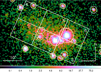
Figure 1: Spectral extraction regions over-plotted on the $3.3-7.5$ keV counts map of M82 for ObsID 10542. The ellipses show the excluded point sources for ObsID 10542. The point source indicated by the letter ’A’ shows the Fe 6.7 keV line and is discussed in §3.2. The dashed panda is the background region adopted for Source A.

Figure 2: Background-subtracted spectra of six box regions combined for all eight observations. The fitting results of the CIE model plus a Gaussian line centered at 6.4 keV are plotted as solid histograms. The fitted Fe 6.4 keV line is indicated as dotted line separately. $\chi$ is the difference between data and model divided by the error.

The background-subtracted spectrum, combined from all eight observations for each region, is plotted in Figure 2. The Fe 6.4 and 6.7 keV lines are clearly seen in most regions. We find the nuclear spectra of M82 within $0.5-7.5$ keV can be fitted with two thermal collisional-ionization-equilibrium (CIE) models with temperatures around 0.65 and $5-6$ keV, respectively. The contribution of the low-temperature component is about 5% around $3-4$ keV and negligible for higher energies. Thus, for the purpose of the study of the Fe 6.4 and 6.7 keV lines, we limit the fitting energy range to $3.3-7.5$ keV and apply only one thermal CIE model (Vapec, Foster et al., 2012) plus a Gaussian line to fit the spectrum. As the Fe lines are the only strong lines in the fitting range, we only fit the Fe abundance in the Vapec model, and the abundances of other elements are fixed to solar values (Lodders, 2003). The Gaussian line is centered at 6.4 keV and its line width is set to a minimum of 10^-6 keV, as it can not be reliablely measured due to the limited instrument resolution. To avoid the contamination of the emission lines of Ar XVII, the energy range between $3.8-4.0$ keV is also ignored. The data are binned to have a minimum count of 25. The spectral analysis is done with the ISIS package (Houck & Denicola, 2000), which calls the Xspec models (Arnaud, 1996).

The fitting results are plotted in Figure 2 and listed in Table 2. From Figure 2 we see that the CIE model plus a Gaussian line generally provides a reasonable fit to the observed spectra. The fitted temperatures are around $5-6$ keV, except for region 6, which may be contaminated by the brightest point source of M82. The fitted Fe abundances are around $0.4-0.6$ times solar value. To measure the intensity of Fe 6.7 keV line, we refit the spectra using a power-law model plus two Gaussian lines centered at 6.4 keV and 6.7 keV, respectively. The fitting results are also listed in Table 2. The fitted power-law indices are around 2. The goodness of the fit for the power-law model is similar to that for the CIE model. The 6.7 keV line is generally stronger than the 6.4 keV line.

Figure 3: Background-subtracted spectrum of the point source A (see Figure 1) that shows the Fe 6.7 keV line. The fitted thermal CIE model is plotted as the solid histogram.

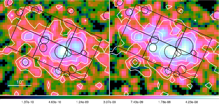
Figure 4: Flux maps of photons within $6.25-6.55$ keV (left) and $6.55-6.85$ keV (right), combined from all eight exposures. A continuum of the linear interpolation of maps of $5.95-6.25$ keV and $6.85-7.15$ keV at 6.4 and 6.7 keV has been subtracted respectively. The exposure-map of the central energy of each band is used when making the flux map. The maps are binned to 0.984 arcsec and smoothed with a two-pixel Gaussian function. The color-bar shows the flux in units of photons^-1cm^-2s^-1pixel^-1. The white contours of the $6.25-6.55$ keV map are plotted in both panels. The extraction regions and excluded sources (black) in Figure 1 are also plotted.

In the fitting above we have neglected the contribution from the unresolved X-ray point sources. Grimm et al. (2003) found that the differential luminosity function of the X-ray point sources in star-forming galaxies follows the form of $N(L_{38})=3.3L_{38}^{-1.6}$SFR, where $L_{38}$ is the $2-10$ keV X-ray luminosity in units of $10^{38}$ erg s^-1 and SFR is the star formation rate measured in units of M_☉ yr^-1. The luminosity of the faintest source in the analysed regions is about $4\times 10^{37}$ erg s^-1 in $3.3-7.5$ keV, which corresponds to $10^{38}$ erg s^-1 in $2-10$ keV for a power-law model with a photon index of 1.8. The adopted SFR of M82 in Grimm et al. (2003) is 3.6 M_☉ yr^-1 based on the H$\alpha$ flux of the entire galaxy. Assuming that half of the X-ray point sources are located at the analysed regions (a fraction estimated from the detected point sources), for unresolved sources between $5\times 10^{35}$ erg s^-1 (the lower limit of the point sources for the luminosity function of Grimm et al. 2003) and $4\times 10^{37}$ erg s^-1 (the lowest luminosity of the detected sources), the contribution to the diffuse emission is about 20%. We test the effect of the unresolved sources by including a power-law model with a photon index of 1.8, the contribution of which is fixed at 20%. The fitted temperatures is a little lower, but still in the ranges obtained without considering the unresolved sources. The Fe abundances are increased by about 20% compared with the results without the power-law model.

3.2 Point sources

We extract the spectra from all individual point sources detected in the nuclear region of M82 and find two sources showing the Fe 6.7 keV line but none showing the Fe 6.4 keV line. One source only appears in the 2010 exposures (ObsID 10545 and 11800) and because its statistics is too low to provide a reliable analysis, it is discarded here. The other one is indicated by the letter ’A’ in Figure 1. It is spatially correlated with the radio source 44.0+59.6 detected by Huang et al. (1994) and is possibly a SNR or a superbubble produced by several SNRs.

The spectrum of Source A is plotted in Figure 3, for which a background extracted from the dashed panda region illustrated in Figure 1 is subtracted. We also fit the spectrum of source A with a CIE model. The fitting result is listed at the bottom row of Table 2. The fitted temperature is 5.8 keV, similar to that measured in the diffuse regions. It corresponds to a shock velocity about 2000 km/s (e.g. Vink, 2012). The flux of source A between 2 and 8 keV is $1.4\times 10^{38}$ erg s^-1. The fitted Fe abundance is 1.7 times solar value, which is about 3 times that of the diffuse regions. Its implications are discussed in §4.

3.3 Imaging analysis

To further illustrate the spatial distribution of the Fe 6.4 and 6.7 keV lines, we plot the flux map of photons within $6.25-6.55$ keV and $6.55-6.85$ keV in Figure 4. We see that both emissions have diffuse morphology and similar spatial extent. The $6.55-6.85$ keV map is slightly more extended along the minor axis of the disk than the $6.25-6.55$ keV map. It is also clear that the two maps do not exactly follow each other and some regions with high $6.25-6.55$ keV flux show less $6.55-6.85$ keV flux.

4 Discussion and Conclusion

We conduct a spatial study of the Fe 6.4 keV and 6.7 keV lines in the nuclear region of M82. The Fe 6.4 keV line is clearly detected with the deep datasets. The emission of both lines have similar spatial extent, but their morphology do not exactly follow each other. The total luminosity of the Fe 6.7 keV line is about $1\times 10^{38}$ erg s^-1, which is consistent with the value measured by Strickland & Heckman (2007). The total luminosity of the Fe 6.4 keV line is about $4\times 10^{37}$ erg s^-1.

The spectra can be fitted well with a CIE model plus a Gaussian line over the energy range of $3.3-7.5$ keV. The fitted temperatures are around $4-6$ keV, which are consistent with the scenario of superwinds (Chevalier & Clegg, 1985). The fitted Fe abundances are around 0.5 solar value. Strickland & Heckman (2007) calculated the Fe abundance produced by SN ejecta and stellar winds using Starburst99 and found 5 times solar abundances. However, the iron may not be well mixed with the hot plasma. The spectrum of the point source A provides an Fe abundance of 1.7 times solar value. Although source A can not be the population of SNRs that are responsible for the present hot gas, if it represents a typical case, then the iron may be depleted heavily. A mild mass-loading of a factor 3 will make the Fe abundance of source A in agreement with that of the hot gas.

As discussed by Strickland & Heckman (2007), the inverse Compton spectrum will have a photon index around 1.3 if the electron population is also responsible for the synchrotron radiation. This index is different from our fitting results of the power-law models, which have photon indices around 2. The contribution of a power-law model of index of 1.3 can not exceed 50%, otherwise it will produce more flux than observed at energies above 7 keV. Adding a power-law model of index of 1.3 to the fit will lower the fitted temperatures. If we require the fitted temperatures to be above 4 keV, the contribution of the inverse Compton emission can not exceed 30%. This is consistent with the contribution fraction of 25% estimated by Strickland & Heckman (2007). Including both the contributions of unresolved point sources and inverse Compton emission will increase the Fe abundances to $0.7-0.9$ solar value, still far below the expected value if there is no depletion of Fe.

We have assumed thermal CIE models when fitting the Fe abundances in §3. The ion at the charge state i approaches to ionization equilibrium on a timescale of $t\sim[n_{e}(C_{i}+\alpha_{i})]^{-1}$, where $n_{e}$ is the electron density, $C_{i}$ is the collisional ionization rate and $\alpha_{i}$ is the recombination rate out of the charge state i (Liedahl, 1999). For a temperature of $6\times 10^{7}$ K, $t\sim 1.5\times 10^{4}n_{e}^{-1}$ yr cm^-3 for the ion of Fe²⁴⁺. The electron density can be estimated from the normalization of Vapec model, which is $\frac{10^{-14}}{4\pi D^{2}}\int n_{e}n_{H}\,dV$, where $D$ (in units of cm) is the distance to M82, $n_{e}$ and $n_{H}$ are the electron and hydrogen densities in units of cm^-3. We adopt a depth of 0.6 kpc, which is the disk spatial extent of the X-ray emitting region of M82. Assuming a filling factor of 1 and $n_{H}=0.8n_{e}$, the electron density $n_{e}\sim 0.35$ cm^-3 for the hot gas in the nuclear region of M82. This gives an ionization equilibrium timescale of $4\times 10^{4}$ yr. It is relatively short compared with the typical timescale ($\sim 10^{6}$ yr) in the starburst region and the outflow timescale ($\sim 5\times 10^{5}$ yr) of the nuclear region of M82. It suggests that non-equilibrium-ionization is unlikely to be important for the Fe 6.7 keV line of M82. When applying a non-equilibrium ionization model (Vnei), we find no improvement in the fits, and it provides a little higher temperature ($7-8$ keV) and a lower Fe abundance.

The Fe 6.4 keV line is the fluorescent line of neutral-like Fe. It has also been observed in another starburst galaxy of NGC 253 (Mitsuishi et al., 2011). They attributed the 6.4 keV line to the irradiation of molecular gas by surrounding point sources. A similar mechanism is applicable for M82, the nuclear region of which contains plenty of cold molecular gases (e.g. Weiß et al., 2001).

The luminosity of all nuclear point sources within $7-8$ keV is about $5\times 10^{39}$ erg s^-1, which is about 15 times the $7-8$ keV luminosity of the diffuse emission and 100 times the luminosity of the Fe 6.4 keV line. The H₂ column densities in the nuclear region of M82 are measured to be around $5\times 10^{22}$ cm^-2 (Weiß et al., 2001). Assuming a solar Fe abundance ($3\times 10^{-5}$ relative to the number of H), the absorption optical depth of the neutral Fe is about 0.1 at 7 keV given an absorption cross-section of $4\times 10^{-20}$ cm² (Veigele, 1973). Taking into account the fluorescence yield of the neutral Fe K line of 0.34 (e.g. Kallman et al., 2004), the observed Fe 6.4 keV line luminosity ($4.5\times 10^{37}$ erg s^-1) is consistent with the irradiation by the hard X-ray photons from nuclear point sources.

References

- Arnaud (1996) Arnaud, K. A. 1996, Astronomical Society of the Pacific Conference Series v101, Astronomical Data Analysis Software and Systems V, ed. Jacoby, G. H. and Barnes, J. 17
- Benson et al. (2003) Benson, A. J., Bower, R. G., Frenk, C. S., Lacey, C. G., Baugh, C. M., Cole, S. 2003, ApJ, 599, 38
- Chevalier & Clegg (1985) Chevalier, R. A. & Clegg, A. W. 1985, Nature, 315, 44
- Foster et al. (2012) Foster, A. R., Ji, L., Smith, R. K. and Brickhouse, N. S. 2012, ApJ, 756, 128
- Grimm et al. (2003) Grimm, H. J., Gilfanov, M.; Sunyaev, R. 2003, MNRAS, 339, 793
- Griffiths et al. (2000) Griffiths, R. E. et al. 2000, Science, 290, 1325
- Houck & Denicola (2000) Houck, J. C. & Denicola, L. A. 2000, in Astronomical Data Analysis Software and Systems IX, eds. N. Manset, C. Veillet, & D. Crabtree, ASP Conf. Ser., 216, 591
- Huang et al. (1994) Huang, Z. P., Thuan, T. X., Chevalier, R. A., Condon, J. J., Yin, Q. F. 1994, ApJ, 424, 114
- Kallman et al. (2004) Kallman, T. R., Palmeri, P., Bautista, M. A., Mendoza, C., Krolik, J. H. 2004, ApJS, 155, 675
- Lehnert & Heckman (1995) Lehnert, M. D. & Heckman, T. M. 1995, ApJS, 97, 89
- Liedahl (1999) Liedahl, D. A. 1999, X-Ray Spectroscopy in Astrophysics, edited by J. V. Paradijs and J. A. M. Bleeker, Lecture Notes in Physics, 520, 189
- Lodders (2003) Lodders, K. 2003, ApJ, 591, 1220
- Mitsuishi et al. (2011) Mitsuishi, I., Yamasaki, N. Y., Takei, Y. 2011, ApJ, 742, L31
- Pettini et al. (2001) Pettini, M., Shapley, A. E., Steidel, C. C., Cuby, J. G., Dickinson, M., Moorwood, A. F. M., Adelberger, K. L., Giavalisco, M. 2001, ApJ, 554, 981
- Songaila (1997) Songaila, A. 1997, ApJ, 490, L1
- Strickland & Heckman (2007) Strickland, D. K. & Heckman, T. M. 2007, ApJ, 658, 258
- Tumlinson et al. (2011) Tumlinson, J. et al. 2011, Sci, 334, 948
- Veigele (1973) Veigele, W. J. 1973, Atomic Data, 5, 51
- Veilleux et al. (2005) Veilleux, S., Cecil, G., Bland-Hawthorn, J. 2005, ARAA, 43, 769
- Vink (2012) Vink, J. 2012, A&ARv, 20, 49
- Weiß et al. (2001) Weiß, A., Neininger, N., Hüttemeister, S., Klein, U. 2001, A&A, 365, 571