Adaptive Mode Selection in Multiuser MISO Cognitive Networks with Limited Cooperation and Feedback

Abstract

In this paper, we consider a multiuser MISO downlink cognitive network coexisting with a primary network. With the purpose of exploiting the spatial degree of freedom to counteract the inter-network interference and intra-network (inter-user) interference simultaneously, we propose to perform zero-forcing beamforming (ZFBF) at the multi-antenna cognitive base station (BS) based on the instantaneous channel state information (CSI). The challenge of designing ZFBF in cognitive networks lies in how to obtain the interference CSI. To solve it, we introduce a limited inter-network cooperation protocol, namely the quantized CSI conveyance from the primary receiver to the cognitive BS via purchase. Clearly, the more the feedback amount, the better the performance, but the higher the feedback cost. In order to achieve a balance between the performance and feedback cost, we take the maximization of feedback utility function, defined as the difference of average sum rate and feedback cost while satisfying the interference constraint, as the optimization objective, and derive the transmission mode and feedback amount joint optimization scheme. Moreover, we quantitatively investigate the impact of CSI feedback delay and obtain the corresponding optimization scheme. Furthermore, through asymptotic analysis, we present some simple schemes. Finally, numerical results confirm the effectiveness of our theoretical claims.

I Introduction

One challenging problem that hinders the further development of wireless communications is the scarcity of available spectrum for the demands of various advanced wireless services. However, FCC’s report shows that the licensed spectrum is heavily underutilized in temporal, frequency or spatial scales [1]. A good solution to solve the above contradiction is the use of cognitive radio (CR) [2] [3]. Generally speaking, a cognitive network is allowed to coexist with a primary network on the licensed spectrum by adaptively adjusting its transmit parameters, i.e., power, time, and frequency, so that the resulting interference to the primary network meets a certain constraint.

Intuitively, the design objective of a CR network is to maximize the spectrum efficiency while satisfying the given interference constraint. Considering the dynamic activity of the primary network, one feasible method is to access the idle spectrum in temporal or frequency scale through effective spectrum sensing [4]-[6]. Clearly, the performance of this method is dependent on the precision of spectrum sensing to a large extent. In fact, it is a passive way for spectrum efficiency improvement, because the spectrum is available only when primary user is inactive. A better method is to find the spectrum availability actively by making use of channel fading, no matter whether the spectrum is idle. As a simple example, the author in [7] proposed to opportunistically control transmit power according to the instantaneous channel state information (CSI), so as to optimize the spectrum efficiency. The key of the realization of active spectrum share lies in exploiting the extra degrees of freedom other than time and frequency. Inspired by interference avoidance through making use of spatial degree of freedom [8] [9], the combination of CR and multiantenna technologies has been proved as an advanced way to achieve the goal of CR in previous literatures [10]-[13]. In this paper, we focus on the design of a multi-antenna transmission scheme for the multiuser MISO cognitive networks under limited CSI feedback.

I-A Related Works

The common to the previous works on multi-antenna cognitive networks lies in how to achieve a balance between increasing the transmission rate of cognitive network and decreasing the interference to primary network. A simplest method to tackle such a challenge is to transmit the signal of cognitive network in the null space of the interference channel from cognitive transmitter to primary receiver. It makes sense only when primary network can not bear any interference. If the interference is bearable within a given constraint, it has been proved that the optimal transmit direction, namely transmit beam, lies in the space spanned jointly by interference channel and the projection of cognitive channel from cognitive transmitter to cognitive receiver into interference channel [14]. Considering the availability of interference CSI may be imperfect, an adaptive beamforming design method coupling with transmission mode selection was proposed, so that the QoS requirement can be fulfilled with the minimum resource consumption [15]. In addition, a robust beamforming method based on mean and covariance information of interference channel was given in [16]. With the purpose of further improving spectrum efficiency, the research focus is shifting from single user to multiuser. The authors in [17] first chose the users whose channels are quasi-orthogonal to interference channel so that the interference are controlled, then a given number of users whose channels are as orthogonal as possible are selected from the above user set, so as to decrease the inter-user interference in cognitive networks. Similarly, an user scheduling scheme was presented to improve the performance of cognitive networks by exploiting the so-called multiuser interference diversity [18]. Furthermore, a joint power control and beamforming strategy was proposed to minimize the total transmit power while satisfying interference constraint to primary users and quality-of-service (QoS) requirements of cognitive users simultaneously [19].

All the above multiantenna schemes can improve spectrum efficiency while meeting interference constraint to some extent. However, they all fend off the question that how multiantenna cognitive transmitter knows the interference CSI. Naturally, the interference CSI is critical to beamforming design and user scheduling at the transmitter. In traditional multiantenna systems, the CSI is usually obtained by limited feedback from the receiver to the transmitter through a quantization codebook [20] [21]. Yet, in cognitive networks, the achievement of the interference CSI needs the cooperation from primary receiver. Inspired by this idea, cooperative feedback from primary receiver to cognitive transmitter was first proposed in [22], so the cognitive transmitter can design the optimal beamformer according to the instantaneous interference CSI. Meanwhile, the authors also gave a detailed discussion on feedback allocation between channel direction information and interference power control information, so as to optimize the performance while meeting the interference constraint. Similarly, based on the cooperative feedback information, the authors in [23] proposed to select the optimal cognitive user, such that the benefit of multiuser diversity can be obtained. Intuitively, the more accurate the CSI at the transmitter, the better the system performance. However, different from traditional multiantenna systems, primary receiver has no obligation to convey the CSI to cognitive transmitter. This is an inevitable problem in cooperative feedback based cognitive networks.

Moreover, transmission mode, namely the number of accessing users, is also an important factor for performance improvement in multiuser multiantenna system [24] [25]. To be precise, a large transmission mode can obtain high spatial multiplexing gain, while it may result in severe inter-user interference. Hence, it is necessary to select the optimal transmission mode according to channel conditions, especially in the case of limited CSI feedback, since the amount of CSI has a great impact on mode selection. In [26], the authors gave a comprehensive performance analysis for a multiuser MISO downlink with limited feedback and feedback delay, then proposed mode switching between single-user (SU) mode and multiuser (MU) mode by comparing the average sum rates for a given SINR. It is worth pointing out this work only considers two transmission mode, name $M=1$ and $M=N_{t}$, where $N_{t}$ is the number of transmit antenna at BS. In multiuser multiantenna cognitive network, mode selection is an effective way of coordinating intra-network (inter-user) and inter-network interference, and thus improve the performance significantly. Yet, mode selection in cognitive network is a more challenging task, since it is affected by intra-network interference and inter-network interference simultaneously, especially when the CSI is imperfect.

I-B Main Contributions

In this paper, we focus on a limited cooperative multiuser MISO cognitive network. In order to let primary receiver help cognitive transmitter of its own accord, we propose that cognitive network purchases partial interference CSI from primary network with an appreciate cost. Therefore, primary network obtains some profits and cognitive network improves its performance, which is a win-win solution. Intuitively, the more the feedback amount, the better the performance, but the higher the feedback cost. For the sake of balancing system performance and feedback cost, it is imperative to design a feedback efficient multiuser transmission scheme. Thereby, we propose a concept of feedback utility function, defined as the difference of the average sum rate of cognitive network and feedback cost. In this paper, we take the maximization of feedback utility function as the optimization objective. As analyzed above, for a multiantenna broadcast channel with limited feedback, the number of accessing users, namely transmission mode, has a great impact on the average sum rate. Hence, in order to maximize the feedback utility function, it is necessary to jointly optimize feedback amount and transmission mode. The main contributions of this paper are summarized as follows

1. We propose a framework of limited cooperative zero-forcing beamforming (ZFBF) for multiuser MISO cognitive networks, so as to mitigate the inter-network and intra-network interferences effectively.

2. We reveal the relationship among the interference, feedback amount, transmit power and number of accessing user, so that the parameters of cognitive network can be adaptively adjusted according to interference constraint.

3. We define a feedback utility function as the difference of the average sum rate of cognitive network and feedback cost. By maximizing the feedback utility function, we get the optimal and suboptimal algorithms that derive the transmission mode and feedback amount.

4. We investigate of the impact of feedback delay on feedback utility function, and obtain analytically the corresponding transmission mode and feedback amount joint optimization scheme.

5. We present some relatively simple optimization schemes in three extreme cases through asymptotic performance analysis.

I-C Paper Organization

The rest of this paper is organized as follows. In Section II, we give a brief overview of the system model and introduce the transmission protocol of cognitive network. Section III focuses on the derivation of the optimal feedback amount and transmission mode by maximizing the feedback utility function while satisfying the interference constraint. Then, the asymptotic characteristics of the performance is analyzed in Section IV. Simulation results are given in Section V to validate the effectiveness of the proposed schemes and we conclude the whole paper in Section VI.

Notation: We use bold upper (lower) letters to denote matrices (column vectors), $(\cdot)^{H}$ to denote conjugate transpose, $E[\cdot]$ to denote expectation, $\|\cdot\|$ to denote the $L_{2}$ norm of a vector, $|\cdot|$ to denote the absolute value, $\lceil a\rceil$ to denote the smallest integer not less than $a$, $\lfloor a\rfloor$ to denote the largest integer not greater than $a$, and $\stackrel{{\scriptstyle d}}{{=}}$ to denote the equality in distribution. The acronym i.i.d means “independent and identically distributed”, pdf means “probability density function” and cdf means “cumulative density function”.

II System Model

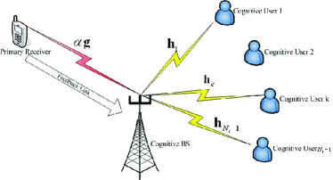
Figure 1: The considered system model.

We consider a system composed of a primary network and a cognitive network, as seen in Fig.1. It is assumed that the two networks share the same spectrum for transmission. The cognitive network includes an $N_{t}$-antenna cognitive base station (BS) and $K$ single-antenna cognitive users. In order to guarantee the normal communication of primary network, the interference from cognitive BS to the single-antenna primary receiver must satisfy a given constraint, which is the precondition that primary network allows cognitive network to access the licensed spectrum. Meanwhile, primary transmitter will interfere with cognitive network. In this paper, we integrate the interference from primary transmitter into the noise at cognitive users, so we omit primary transmitter in this system. Note that this paper focuses on mode selection but not user scheduling, we fix the user number $K=N_{t}-1$ because at most $N_{t}-1$ users are allowed to access cognitive network while one spatial degree of freedom of $N_{t}$-antennas cognitive BS is used for interference suppression. In practical network, if $K$ is large, we can combine space division multiplexing access (SDMA) with time division multiplexing access (TDMA). Specifically, cognitive users can access the network in different time slots based on some user scheduling schemes.

It is assumed that the downlink is homogenous, where cognitive users have the same channel vector statistics, same path loss and same receive noise variance. The channels $\textbf{h}_{k},k=1,\cdots,N_{t}-1$ from cognitive BS to cognitive users are $N_{t}$ dimensional i.i.d Gaussian random vectors with zero mean and unit variance, and the path loss is normalized to 1. The path loss component of interference channel from cognitive BS to primary receiver is $\alpha$ with respect to that of downlink channel, and small scale fading component g is also an $N_{t}$ dimensional circular symmetrical complex Gaussian random vector. Considering path loss varies slowly and is a scalar, we assume cognitive BS knows $\alpha$ fully through the aid of a positioning system and the amount of exchange information can be neglected. Cognitive network communicates in the form of time slot, and all the channels are assumed to keep constant during one time slot and fade independently slot by slot. At the beginning of each time slot, primary receiver and cognitive users convey the corresponding CSI to cognitive BS based on quantization codebooks. All the codebooks are designed in advance and stored at the transmitter and the receivers. Assuming the codebook of size $2^{B}$ at primary receiver is $\mathcal{G}=\{\hat{\textbf{g}}_{1},\cdots,\hat{\textbf{g}}_{2^{B}}\}$, which is a collection of unit norm vectors, then the optimal quantization codeword selection criterion can be expressed as

$$i=\arg\max\limits_{1\leq j\leq 2^{B}}|\hat{\textbf{g}}_{j}^{H}\tilde{\textbf{g}}|^{2},$$ (1)

where $\tilde{\textbf{g}}=\frac{\textbf{g}}{\|\textbf{g}\|}$ is the channel direction vector. Specifically, index $i$ is conveyed by primary receiver and $\hat{\textbf{g}}_{i}$ is recovered at cognitive BS as instantaneous CSI of the interference channel. The quantization codebook of size $2^{C}$ at cognitive user $k$ is $\mathcal{H}_{k}=\{\hat{\textbf{h}}_{k,1},\cdots,\hat{\textbf{h}}_{k,2^{C}}\},k=1,\cdots,N_{t}-1$, and the same process of codeword selection, index conveyance and CSI recovery is used to help cognitive BS to obtain CSI of downlink channels. It is worth pointing out that the feedback amount $C$ is fixed and $B$ is dynamically variable as discussed below.

Based on the feedback information from primary receiver and cognitive users, cognitive BS determines the optimal transmit beam of the $m$th user of the selected $M$ users $\textbf{w}_{K_{m}},m=1,\cdots,M,1\leq M\leq N_{t}-1$ by making use of zero-forcing beamforming design methods, when given transmission mode $M$. Specifically, for $\hat{\textbf{h}}_{K_{m}}$, the complementary channel matrix is

$$\bar{\hat{\textbf{H}}}_{K_{m}}=[\hat{\textbf{g}},\hat{\textbf{h}}_{K_{1}},\cdots,\hat{\textbf{h}}_{K_{m-1}},\hat{\textbf{h}}_{K_{m+1}},\cdots,\hat{\textbf{h}}_{K_{M}}].$$

Taking singular value decomposition (SVD) to $\bar{\hat{\textbf{H}}}_{K_{m}}$, if $\textbf{V}_{K_{m}}^{\perp}$ is the matrix composed of the right singular vectors related to zero singular values, then we randomly choose a unit norm vector from the space spanned by $\textbf{V}_{K_{m}}^{\perp}$ as the transmit beam $\textbf{w}_{K_{m}}$. Since $\textbf{V}_{K_{m}}^{\perp}$ is the null space of $\bar{\hat{\textbf{H}}}_{K_{m}}$, we have

$$\hat{\textbf{g}}^{H}\textbf{w}_{K_{m}}=0,$$ (2)

and

$$\hat{\textbf{h}}_{K_{k}}^{H}\textbf{w}_{K_{m}}=0,$$ (3)

where $1\leq k\leq M,k\neq m$. Thus, the receive signal at the $K_{m}$th user can be expressed as

$$y_{K_{m}}=\sqrt{\frac{P}{M}}\textbf{h}_{K_{m}}^{H}\sum\limits_{k=1}^{M}\textbf{w}_{K_{k}}x_{K_{k}}+n,$$ (4)

where $x_{K_{m}}$ the normalized transmit signal related to the $K_{k}$th user, $y_{K_{m}}$ is the receive signal at the $K_{m}$th user, $P$ is the total transmit power of cognitive BS, which is distributed to $M$ users equally, and $n$ is additive white Gaussian noise with zero mean and variance $\sigma^{2}$. Then, the interference from cognitive BS to primary receiver, and the receive signal to interference and noise ratio (SINR) at cognitive user $K_{m}$ are given by

$$I=P/M\alpha\sum\limits_{m=1}^{M}|\textbf{g}^{H}\textbf{w}_{K_{m}}|^{2},$$ (5)

and

$$SINR_{K_{m}}=\frac{|\textbf{h}_{K_{m}}^{H}\textbf{w}_{K_{m}}|^{2}}{\sigma^{2}M/P+\sum\limits_{k=1,k\neq m}^{M}|\textbf{h}_{K_{m}}^{H}\textbf{w}_{K_{k}}|^{2}},$$ (6)

respectively.

The precondition that cognitive network is allowed to access the licensed spectrum is that the interference from cognitive BS to primary receiver meets a given constraint. Average interference constraint (AIC) and peak interference constraint (PIC) are two commonly used interference conditions in cognitive networks. Previous works have proved that from the view of throughput maximization, given the same average and peak interference constraints, the AIC is more favorable than the PIC because of its more flexibility for dynamically allocating transmit powers over different fading states [27] [28], thus we take the AIC as the constraint condition in this paper. If $\bar{I}_{\textrm{AIC}}$ is the allowable maximum average interference, the interference constraint is given by

$$\bar{I}=E[I]\leq\bar{I}_{\textrm{AIC}}.$$ (7)

Intuitively, when $\bar{I}_{\textrm{AIC}}$ is given, the available maximum transmit power $P$ increases with the increase of feedback amount $B$, and thus the performance of cognitive network improves accordingly, but the feedback cost also increases. In order to achieve a tradeoff between the performance and feedback cost, we take the maximization of feedback utility function as the optimization objective, which is defined as

$$f(M,B)$$

$$= E\Bigg{[}\sum\limits_{m=1}^{M}\log_{2}\left(1+\frac{|\textbf{h}_{K_{m}}^{H}\textbf{w}_{K_{m}}|^{2}}{\sigma^{2}M/P+\sum\limits_{k=1,k\neq m}^{M}|\textbf{h}_{K_{m}}^{H}\textbf{w}_{K_{k}}|^{2}}\right)$$

$$- \mu B\Bigg{]}$$

$$= ME\left[\log_{2}\left(1+\frac{|\textbf{h}_{K_{1}}^{H}\textbf{w}_{K_{1}}|^{2}}{\sigma^{2}M/P+\sum\limits_{k=2}^{M}|\textbf{h}_{K_{1}}^{H}\textbf{w}_{K_{k}}|^{2}}\right)\right]-\mu B,$$

where (LABEL:eqn9) holds true since the $SINR$s of the users are i.i.d. $\mu$ is the pricing factor of feedback information from the primary receiver whose unit is rate penalty per feedback bit. $\mu$ is depending on cooperative cost, mainly including power and spectrum consumption for channel estimation, codeword selection and index feedback, and is determined based on a negotiation or competition scheme between cognitive and primary networks, such as stackelberg game [29]. Generally speaking, if primary network asks for a higher unit price, cognitive network will purchase less feedback information, resulting in low profits. The optimal $\mu$ will be determined when one side can not further improve its utility, if the other side’s utility is not deceased. Once the price is determined, the owner of cognitive network will pay the owner of primary network. Thus, these two networks can get some profits from cooperative feedback. In this paper, we concentrate on the optimization of feedback utility, so we assume the pricing factor has been determined by the two sides based on a certain method, such as stackelberg game. As seen in (LABEL:eqn9), feedback utility function is a function of $B$ and $M$. In order to maximize feedback utility function, it is necessary to jointly optimize the two variables. Hence, the focus of this paper is on the joint optimization of feedback amount $B$ and transmission mode $M$ by maximizing feedback utility function (LABEL:eqn9) while satisfying AIC.

III Adaptive Mode Selection

As mentioned earlier, this paper focuses on the maximization of the feedback utility function while satisfying AIC through adaptive mode selection and dynamic feedback control. As seen in (5), given a channel condition $\alpha$, the interference $I$ is a function of transmit power $P$, transmission mode $M$ and feedback amount $B$. Hence, when $I$ is given, there is a tradeoff among $P$, $M$ and $B$. On the other hand, it is known from (6) that, $P$ and $M$ also have a great impact on the receive SINR, and thus the feedback utility function. Therefore, prior to discussing the optimal transmission mode $M$, we need to reveal the relationship among the interference, feedback utility function, transmit power, feedback amount and transmission mode.

By using ZFBF based on limited feedback information from primary receiver, the relation between the residual AIC, transmit power, transmission mode and feedback amount is given by

Theorem 1: Given $P$ and $B$, the residual AIC at primary receiver after ZFBF is tightly upper bounded by $\frac{\alpha PN_{t}}{N_{t}-1}2^{-\frac{B}{N_{t}-1}}$.

Proof:

Following the theory of random vector quantization (RVQ) [30], the relationship between the original and the quantized channel direction vectors can be expressed as

$$\tilde{\textbf{g}}=\sqrt{1-a}\hat{\textbf{g}}+\sqrt{a}\textbf{s},$$ (9)

where $\hat{\textbf{g}}$ is the optimal quantization codeword based on codeword selection criterion (1), $a=\sin^{2}\left(\angle\left(\tilde{\textbf{g}},\hat{\textbf{g}}\right)\right)$ is the magnitude of the quantization error, and s is an unit norm vector isotropically distributed in the nullspace of $\hat{\textbf{g}}$, and is independent of $a$. Therefore, the $m$th term of the sum in the right hand side (RHS) of (5) is derived as

$$|\tilde{\textbf{g}}^{H}\textbf{w}_{K_{m}}|^{2} = \left|\sqrt{1-a}\hat{\textbf{g}}^{H}\textbf{w}_{K_{m}}+\sqrt{a}\textbf{s}^{H}\textbf{w}_{K_{m}}\right|^{2}$$ (10)

$$= a|\textbf{s}^{H}\textbf{w}_{K_{m}}|^{2},$$

where (10) follows from the fact that $\textbf{w}_{K_{m}}$ is in the nullspace of $\hat{\textbf{g}}$, namely $\hat{\textbf{g}}^{H}\textbf{w}_{K_{m}}=0$. Due to the independence of channel magnitude component and channel direction component, the AIC is reduced to

$$\bar{I} = \alpha P/M\sum\limits_{m=1}^{M}E[\|\textbf{g}\|^{2}]E[a]E[|\textbf{s}^{H}\textbf{w}_{K_{m}}|^{2}]$$ (11)

$$= \alpha PE[\|\textbf{g}\|^{2}]E[a]E[|\textbf{s}^{H}\textbf{w}_{K_{1}}|^{2}],$$

where (11) holds true because $|\textbf{s}^{H}\textbf{w}_{K_{m}}|^{2}$ is i.i.d. for $m=1,\cdots,M$. Hence, in order to obtain $\bar{I}$, we only need to compute the three expectation terms. First, since $\|\textbf{g}\|^{2}$ is $\chi^{2}(2N_{t})$ distributed, we have $E[\|\textbf{g}\|^{2}]=N_{t}$. As we known, $a=1-|\hat{\textbf{g}}^{H}\tilde{\textbf{g}}|^{2}$. For an arbitrary quantization codeword $\hat{\textbf{g}}_{j}$, $1-|\hat{\textbf{g}}_{j}^{H}\tilde{\textbf{g}}|^{2}$ is $\beta(N_{t}-1,1)$ distributed [30], so that $a$ is the minimum of $2^{B}$ independent $\beta(N_{t}-1,1)$ random variable, and thus its expectation can be tightly upper bounded as $E[a]<2^{-\frac{B}{N_{t}-1}}$. Finally, since s and $\textbf{w}_{K_{1}}$ are i.i.d. isotropic vectors in the $(N_{t}-1)$ dimensional nullspace of $\hat{\textbf{g}}$, $|\textbf{s}^{H}\textbf{w}_{K_{1}}|^{2}$ is $\beta(1,N_{t}-2)$ distributed [30], whose expectation is equal to $\frac{1}{N_{t}-1}$. As a result, we have $\bar{I}<\frac{\alpha PN_{t}}{N_{t}-1}2^{-\frac{B}{N_{t}-1}}$ ∎

According to Theorem 1, given AIC $I_{\textrm{AIC}}$, feedback amount $B$ and transmit mode $M$, in order to meet AIC strictly, transmit power $P$ has an upper bound

$$P=\frac{(N_{t}-1)I_{\textrm{AIC}}}{\alpha N_{t}}2^{\frac{B}{N_{t}-1}}.$$ (12)

Substituting (12) into (LABEL:eqn9), we have

$$f(M,B)$$ (13)

$$= ME\left[\log_{2}\left(1+\frac{|\textbf{h}_{K_{1}}^{H}\textbf{w}_{K_{1}}|^{2}}{\eta M2^{-\frac{B}{N_{t}-1}}+\sum\limits_{k=2}^{M}|\textbf{h}_{K_{1}}^{H}\textbf{w}_{K_{k}}|^{2}}\right)\right]$$

$$- \mu B,$$

where $\eta=\frac{\alpha N_{t}\sigma^{2}}{(N_{t}-1)I_{\textrm{AIC}}}$. Clearly, the key of obtaining $f(M,B)$ is to compute the average rate of the $K_{m}$th cognitive user. Before computing the average rate, we need to know the pdf of the receive $SINR$. Examining the receive $SINR_{K_{1}}$, it is upper bounded by

$$SINR_{K_{1}} = \frac{|\textbf{h}_{K_{1}}^{H}\textbf{w}_{K_{1}}|^{2}}{\eta M2^{-\frac{B}{N_{t}-1}}+\sum\limits_{k=2}^{M}|\textbf{h}_{K_{1}}^{H}\textbf{w}_{K_{k}}|^{2}}$$ (14)

$$= \frac{\|\textbf{h}_{K_{1}}\|^{2}|\tilde{\textbf{h}}_{K_{1}}^{H}\textbf{w}_{K_{1}}|^{2}}{\eta M2^{-\frac{B}{N_{t}-1}}+\|\textbf{h}_{K_{1}}\|^{2}b\sum\limits_{k=2}^{M}|\textbf{s}^{H}\textbf{w}_{K_{k}}|^{2}}$$

$$\stackrel{{\scriptstyle d}}{{=}} \frac{\|\textbf{h}_{K_{1}}\|^{2}\beta(1,N_{t}-1)}{\eta M2^{-\frac{B}{N_{t}-1}}+\|\textbf{h}_{K_{1}}\|^{2}b\sum\limits_{k=2}^{M}\beta(1,N_{t}-2)}$$ (15)

$$\stackrel{{\scriptstyle d}}{{=}} \frac{\|\textbf{h}_{K_{1}}\|^{2}\beta(1,N_{t}-1)}{\eta M2^{-\frac{B}{N_{t}-1}}+\sum\limits_{k=2}^{M}\Gamma(N_{t}-1,\delta)\beta(1,N_{t}-2)}$$

$$\stackrel{{\scriptstyle d}}{{=}} \frac{\chi_{2}^{2}}{\eta M2^{-\frac{B}{N_{t}-1}}+\delta\chi_{2(M-1)}^{2}}$$

where $b=\sin^{2}(\angle(\tilde{\textbf{h}}_{K_{1}},\hat{\textbf{h}}_{K_{1}}))$ and $\delta=2^{-\frac{C}{N_{t}-1}}$. (14) holds true because $\tilde{\textbf{h}}_{K_{1}}=\sqrt{1-b}\hat{\textbf{h}}_{K_{1}}+\sqrt{b}\textbf{s}$ and $\hat{\textbf{h}}_{K_{1}}^{H}\textbf{w}_{K_{k}}=0$, (15) follows from the fact that $|\tilde{\textbf{h}}_{K_{1}}^{H}\textbf{w}_{K_{1}}|^{2}$ and $|\textbf{s}^{H}\textbf{w}_{K_{k}}|^{2}$ are $\beta(1,N_{t}-1)$ and $\beta(1,N_{t}-2)$ distributed as analyzed in (11), and (III) is derived since $\|\textbf{h}_{K_{1}}\|^{2}b$ is $\Gamma(N_{t}-1,\delta)$ distributed according to the theory of quantization cell approximation [31]. For the product of a $\Gamma(N_{t}-1,\delta)$ distributed random variable and a $\beta(1,N_{t}-2)$ distributed random variable, it is equal to $\delta\chi_{2}^{2}$ in distribution [26]. Based on the fact that the sum of $M-1$ independent $\chi_{2}^{2}$ distributed random variables is $\chi_{2(M-1)}^{2}$ distributed, $SINR_{K_{1}}$ is equal to $\frac{\chi_{2}^{2}}{\eta M2^{-\frac{B}{N_{t}-1}}+\delta\chi_{2(M-1)}^{2}}$ in distribution. Let $y\sim\chi_{2(N_{t}-1)}^{2}$ and $z\sim\chi_{2}^{2}$, we can derive the cdf and pdf of $SINR_{K_{m}}$ as

$$P(x) = P\left(\frac{z}{\eta M2^{-\frac{B}{N_{t}-1}}+\delta y}\leq x\right)$$ (17)

$$= \int_{0}^{\infty}F_{Z|Y}\big{(}x(\eta M2^{-\frac{B}{N_{t}-1}}+\delta y)\big{)}f_{Y}(y)dy$$

$$= \int_{0}^{\infty}\big{(}1-\exp(-x(\eta M2^{-\frac{B}{N_{t}-1}}+\delta y))\big{)}$$

$$\times \frac{y^{M-2}}{\Gamma(M-1)}\exp(-y)dy$$

$$= 1-\frac{\exp\left(-\eta M2^{-\frac{B}{N_{t}-1}}x\right)}{\left(1+\delta x\right)^{M-1}}$$

$$\times \int_{0}^{\infty}\frac{\exp(-(1+\delta x)y)((1+\delta x)y)^{M-2}}{\Gamma(M-1)}d((1+\delta x)y)$$

$$= 1-\frac{\exp\left(-\eta M2^{-\frac{B}{N_{t}-1}}x\right)}{\left(1+\delta x\right)^{(M-1)}},$$

and

$$p(x) = \eta M2^{-\frac{B}{N_{t}-1}}\exp\left(-\eta M2^{-\frac{B}{N_{t}-1}}x\right)\left(1+\delta x\right)^{-(M-1)}$$ (18)

$$- \delta(N_{t}-1)\exp\left(-\eta M2^{-\frac{B}{N_{t}-1}}x\right)\left(1+\delta x\right)^{-M},$$

respectively, where $F_{Z|Y}(\cdot)$ is the conditional cdf of $z$ for a given $y$, $f_{Y}(\cdot)$ is the pdf of $y$, $\Gamma(\cdot)$ is the Gamma function. (17) holds true because $\frac{\exp(-(1+\delta x)y)((1+\delta x)y)^{M-2}}{\Gamma(M-1)}$ is the pdf of $(1+\delta x)y$. Hence, $f(M,B)$ can be casted as

$$f(M,B)$$ (19)

$$= M\int_{0}^{\infty}\log_{2}\left(1+x\right)p(x)dx-\mu B$$

$$\approx M\log 2(e)E\left[\ln(1+x)\right]-\mu B$$

$$= M\log 2(e)\int_{0}^{\infty}\frac{1-P(x)}{x+1}dx-\mu B$$

$$= \frac{\log_{2}(e)M}{\delta^{M-1}}\int_{0}^{\infty}\frac{\exp\left(-\eta M2^{-\frac{B}{N_{t}-1}}x\right)}{(x+1)(x+\delta^{-1})^{M-1}}dx-\mu B$$

$$= \frac{\log_{2}(e)M}{\delta^{M-1}}I_{1}\left(\eta M2^{-\frac{B}{N_{t}-1}},\delta^{-1},M-1\right)-\mu B,$$

where

$$I_{1}(x,y,z) = \int_{0}^{\infty}\frac{\exp\left(-xt\right)}{(t+1)(t+y)^{z}}dt$$

$$= \sum\limits_{i=1}^{z}(-1)^{i-1}(1-y)^{-i}I_{2}(x,y,z-i+1)$$

$$+ (y-1)^{-z}I_{2}(x,1,1),$$

and

$$I_{2}(x,y,z)=\left\{\begin{array}[]{ll}\exp(xy)\textmd{E}_{1}(xy)&z=1\\ \sum\limits_{k=1}^{z-1}\frac{(k-1)!}{(z-1)!}\frac{(-x)^{z-k-1}}{y^{k}}\\ +\frac{(-x)^{z-1}}{(z-1)!}\exp(xy)E_{1}(xy)&z\geq 2\end{array}\right.$$

and $\textmd{E}_{1}(x)$ is the exponential-integral function of the first order.

So far, we have derived the closed-form expression of feedback utility function $f(M,B)$ as a function of $M$ and $B$. Then, the joint optimization of $M$ and $B$ is equivalent to the following optimization problem:

$$J_{1}:\max\limits_{M,B} f(M,B)$$

$$s.t.\quad 2\leq M\leq N_{t}-1$$

$$B\leq B_{0},$$

where $B_{0}$ is the maximum usable feedback amount considering the complexity of codebook design and codeword selection in practical networks. $M$ must be greater than $1$ because $M=1$ is unsuitable for ZFBF. Since both $M$ and $B$ are integers, $J_{1}$ is an integer programming problem, so it is difficult to get the closed-form expressions of $M$ and $B$. Considering $M$ and $B$ are upper bounded by $N_{t}-1$ and $B_{0}$ respectively, which are impossibly to be large values in practical networks. Thereby, for each transmission mode, we could derive the optimal feedback bits and the corresponding feedback utility function. Among all $(M,B)$ combinations, it is easy to get the optimal one with the maximum feedback utility function. Thus, the whole procedure can be summarized as below.

 

Optimal Algorithm

1. Initialization: given $N_{t}$, $\mu$, $\alpha$, $B_{0}$, $C$ and $I_{\textrm{AIC}}$. Set $M=2$, $B=0$, $i=1$ and $j=1$.

2. Let $M_{i}=M$, $B_{j}=B$, and compute $f_{i,j}=f(M,B)$.

3. If $B+1\leq B_{0}$, then $B=B+1$, $j=j+1$, and go to 2).

4. If $M+1\leq N_{t}-1$, then $M=M+1$, $i=i+1$, $B=0$, $j=1$ and go to 2).

5. Search $(n^{*},m^{*})=\arg\min\limits_{1\leq n\leq i,1\leq m\leq j}f_{n,m}$. $M_{n^{*}}$ and $B_{m^{*}}$ are the optimal transmission mode and feedback amount, respectively.

 

Clearly, the optimal algorithm essentially is a numerical search method with high complexity. Herein, we give a suboptimal algorithm with low complexity to derive the $(M,B)$ combination. As mentioned earlier, one of the difficulties to solve the above problem lies in that both $M$ and $B$ are integers. If we relax the two constraints, we may reduce the solving complexity. In this context, $J_{1}$ is transformed as the following general optimization problem

$$J_{2}:\max\limits_{M,B} f(M,B)$$

$$s.t.\quad 2\leq M\leq N_{t}-1$$

$$B\leq B_{0}$$

$$M\in\mathbf{R}^{+}$$

$$B\in\mathbf{R}^{+},$$

where $\mathbf{R}^{+}$ is the collection of the positive real value. $J_{2}$ is a nonlinear programming (NLP) problem with linear constraints. At present, a commonly used method to solve such a problem is sequential linear programming (SLP). SLP consists of linearizing the objective in a region around a nominal operating point by a Taylor series expansion. The resulting linear programming problem is then solved by standard methods such as the interior point method. Some softwares, i.e. Lingo and Matlab, usually solve the NLP problem by SLP, so we can use them to resolve $J_{2}$ directly. Assuming $(M^{{\dagger}},B^{{\dagger}})$ is the solution to $J_{2}$. Let $M_{1}=\lceil M^{{\dagger}}\rceil$ and $M_{2}=\lfloor M^{{\dagger}}\rfloor$ be the candidate transmission modes, and $B_{1}=\lceil B^{{\dagger}}\rceil$ and $B_{2}=\lfloor B^{{\dagger}}\rfloor$ be the candidate feedback amounts. Then, select the combination that has the maximum feedback utility function from $(M_{1},B_{1})$, $(M_{1},B_{2})$, $(M_{2},B_{1})$ and $(M_{2},B_{2})$ as the solution to the original optimization problem. Although the solution of this algorithm may not be optimal, it can achieve a tradeoff between the performance and computation complexity. With respect to the optimal numerical searching algorithm mentioned above, which needs to compare $(N_{t}-2)(B_{0}+1)$ feedback utility functions, the proposed algorithm has a quite low complexity, especially when $N_{t}$ and $B_{0}$ are large. It is worth pointing out that this algorithm is performed only when channel condition $\alpha$ varies, but not during each time slot, so it can be run offline.

Remark1: In this paper, we consider the case with one primary user. Actually, the proposed scheme can generalize to the case of multiple primary users directly. The impact of multiple primary users lies in three folds. First, assuming there are $L$ primary users, the maximum transmission mode is $N_{t}-L$, because $L$ spatial degrees of freedom is used to mitigate the interferences to $L$ primary users. In other words, if $L\geq N_{t}$, no cognitive user is allowed to access the licensed spectrum. Second, transmit power is constrained by $L$ interference channels simultaneously. For simplicity, assuming cognitive BS purchases the same feedback amount $B$ from all $L$ primary users, transmit power is upper bounded by the interference channel that has the largest path loss $\alpha$. Third, cognitive BS needs to purchase feedback from $L$ primary users. The feedback cost increases linearly with $L$ and the average sum rate decreases due to the decrease of spatial degree of freedom, so the maximum feedback utility function may become negative. Under this condition, cognitive network may be unwilling to use this spectrum.

Remark2: The proposed scheme also can be generalized to the case of variable $N_{t}$ by taking $N_{t}$ as an optimization variable, so that the performance of cognitive network may be further improved. Under this condition, the focused problem in this paper becomes a subproblem of the whole optimization problem. since $N_{t}$ is an integer variable, we can first derive all the combinations of $M$ and $B$ when scaling $N_{t}$ from $2$ to the number of antennas at cognitive BS minus $L$ by the proposed scheme. Then, find the optimal combination $(M,B)$ with the maximum feedback utility function, the corresponding $N_{t}$ is the optimal antenna number.

Due to relatively long distance between primary receiver and cognitive BS, there may be more or less feedback delay during quantized CSI conveyance, resulting in CSI mismatch when designing ZFBF, and thus interference constraint may be unsatisfied if outdated CSI is used directly. Herein, we give an investigation of the impact of feedback delay on feedback utility function and then present a robust mode selection scheme based on limited feedback. Following [32], we model the CSI as

$$\textbf{g}_{r}=\sqrt{\rho}\textbf{g}_{o}+\sqrt{1-\rho}\textbf{e},$$ (20)

where $\textbf{g}_{r}$ and $\textbf{g}_{o}$ are the real and the outdated CSI, respectively. e is the error vector due to feedback delay with i.i.d. zero mean and unit variance complex Gaussian entries, and $\rho$ is the correlation coefficient, which is dependent of normalized frequency shift and delay duration. Clearly, the larger the correlation coefficient $\rho$, the less the CSI mismatch. Substituting (20) into (5), the interference term is transformed as

$$I = P/M\alpha\sum\limits_{m=1}^{M}|\textbf{g}_{r}^{H}\textbf{w}_{K_{m}}|^{2}$$ (21)

$$= P/M\alpha\sum\limits_{m=1}^{M}|\sqrt{\rho}\textbf{g}_{o}^{H}\textbf{w}_{K_{m}}+\sqrt{1-\rho}\textbf{e}^{H}\textbf{w}_{K_{m}}|^{2}$$

$$= P/M\alpha\sum\limits_{m=1}^{M}|\sqrt{a\rho}\textbf{s}^{H}\textbf{w}_{K_{m}}+\sqrt{1-\rho}\textbf{e}^{H}\textbf{w}_{K_{m}}|^{2}.$$

Under this condition, the average AIC can be computed as

$$\bar{I} = P\alpha E\left[|\sqrt{a\rho}\textbf{s}^{H}\textbf{w}_{K_{m}}+\sqrt{1-\rho}\textbf{e}^{H}\textbf{w}_{K_{m}}|^{2}\right]$$ (22)

$$= P\alpha\left(E\left[a\rho|\textbf{s}^{H}\textbf{w}_{K_{m}}|^{2}\right]+E\left[(1-\rho)|\textbf{e}^{H}\textbf{w}_{K_{m}}|^{2}\right]\right)$$

$$< P\alpha\left(\frac{N_{t}\rho}{N_{t}-1}2^{-\frac{B}{N_{t}-1}}+(1-\rho)\right)$$

$$= \frac{\alpha PN_{t}}{N_{t}-1}2^{-\frac{B}{N_{t}-1}}\left(1+\left(1-\rho\right)\left(\frac{N_{t}-1}{N_{t}}2^{\frac{B}{N_{t}-1}}-1\right)\right),$$

where (22) holds true because s and e are independent of each other, (III) following from the fact that $|\textbf{e}^{H}\textbf{w}_{K_{m}}|^{2}$ is $\chi_{2}^{2}$ distributed and $E\left[|\textbf{e}^{H}\textbf{w}_{K_{m}}|^{2}\right]=1$. Notice that the average interference without CSI mismatch is $\frac{\alpha PN_{t}}{N_{t}-1}2^{-\frac{B}{N_{t}-1}}$, if $\frac{N_{t}-1}{N_{t}}2^{\frac{B}{N_{t}-1}}>1$, the CSI mismatch leads to the increase of average interference. In other words, with the same average interference constraint and feedback amount, the available maximum transmit power decreases accordingly due to CSI mismatch. Otherwise, if $(N_{t}-1)/N_{t}2^{B/(N_{t}-1)}<1$, the CSI mismatch will decrease the average interference, so that cognitive BS can use higher transmit power to improve the performance. Hence, the upper bound of transmit power in presence of delay while satisfying AIC can be expressed as

$$P=\frac{I_{\textrm{AIC}}}{\alpha\left(\frac{N_{t}\rho}{N_{t}-1}2^{-\frac{B}{N_{t}-1}}+(1-\rho)\right)}.$$ (25)

Substituting (25) into (LABEL:eqn9), we can derive the feedback utility function in presence of feedback delay, and thus the corresponding optimal $B$ and $M$ can be obtained by using the above proposed algorithm.

IV Asymptotic Analysis

In this section, for the sake of deriving the optimal $(M,B)$ and evaluating the performance easily, we analyze the asymptotic characteristics of feedback utility function in some extreme cases.

IV-A High AIC and/or Small $\alpha$

If primary receiver can bear sufficiently high AIC and/or $\alpha$ is sufficiently small due to large distance between cognitive BS and primary receiver, such that AIC can still be met even with $B=0$ and arbitrarily high transmit power. Under such a condition, it is clear that $B=0$ is optimal in the sense of maximizing feedback utility function. In other words, without the help from primary receiver, cognitive network can work freely. It is equivalent to the traditional mode selection on broadcast channel. Assuming a certain transmit power $P^{{}^{\prime}}$ is used at cognitive BS, the optimal transmission mode is determined based on the average sum rate of cognitive users

$$R(M)=\frac{M\log_{2}(e)}{\delta^{M-1}}I_{3}\left(\sigma^{2}M/P^{{}^{\prime}},\delta^{-1},M-1\right).$$ (26)

Due to the complex expression, numerical search method is also used to derive the optimal $M$. However, because of only one searching variable, the computation complexity can be reduced significantly.

IV-B Low AIC and/or Large $\alpha$

In the case that primary receiver has a quite strict constraint on AIC and/or $\alpha$ is sufficiently large, the second term of the denominator in (14) can be neglected compared to the first one. Hence, $SINR_{K_{m}}$ is reduced to

$$SINR_{K_{m}}=\frac{\|\textbf{h}_{K_{m}}\|^{2}\beta(1,N_{t}-1)}{\eta 2^{-\frac{B}{N_{t}-1}}},$$ (27)

and the corresponding pdf is

$$p(x)=\eta M2^{-\frac{B}{N_{t}-1}}\exp\left(-\eta M2^{-\frac{B}{N_{t}-1}}x\right).$$ (28)

Therefore, the feedback utility function under this condition can be computed as

$$f(M,B) = M\int_{0}^{\infty}\log_{2}\left(1+x\right)p(x)dx-\mu B$$ (29)

$$= M\log_{2}(e)\exp\left(\eta M2^{-\frac{B}{N_{t}-1}}\right)E_{1}\left(\eta M2^{-\frac{B}{N_{t}-1}}\right)$$

$$- \mu B.$$

It is known from (29) that, $f(M,B)$ is a monotone increasing function of $M$, so that $M=N_{t}-1$ is optimal. On the other hand, $f(M,B)$ is a monotone decreasing function of $B$, then $B=0$ is optimal. In fact, this case is equivalent to a noise-limited system, the help from primary receiver makes no sense and full multiplexing $(M=N_{t}-1)$ is propitious to improve the sum rate, so that it is reasonable to choose $B=0$ and $M=N_{t}-1$.

IV-C Large C

When $C$ is quite large, but still fixed, $b=\sin^{2}(\angle(\tilde{\textbf{h}}_{K_{m}},\check{\textbf{h}}_{K_{m}}))\approx 0$. In other words, the inter-user interference can be neglected. Under this condition, $SINR_{K_{m}}$ has the same expression as (27), so that $M=N_{t}-1$ and $B=0$ are optimal.

V Numerical Results

To examine the effectiveness of the proposed feedback efficient adaptive mode selection scheme in limited cooperative multiuser cognitive networks, we present several numerical results in different scenarios. For all scenarios, we set $N_{t}=5$ considering the maximum number of BS antennas in LTE-A is 8, $B_{0}=4$ due to the complexity constraint on codeword selection at primary receiver, and $\sigma^{2}=1$. Additionally, we use FUF${}_{\textrm{max}}$ to denote the maximum feedback utility function when selecting the optimal transmission mode $M_{\textrm{opt}}$ and feedback bits $B_{\textrm{opt}}$, and use OA and SA to denote the optimal and suboptimal algorithms, respectively. Interestingly, it is found that the suboptimal algorithm has the same optimization results as the optimal one in all scenarios, so that we could replace the optimal algorithm with the suboptimal one in practical networks.

First, we testify the validity of the theoretical claims through numerical simulation with different path losses. In this case, we fix $C=2$ and $\mu=0.1$ for convenience. As seen in Fig.2, in the whole region of interference constraint, the theoretical and simulation results are quite identical. Especially when $I_{\textrm{AIC}}<-10$dB, the two ones are nearly coincident for different path losses. Meanwhile, it is found that path loss $\alpha$ has a great impact on mode selection and feedback bits, and thus maximum feedback utility function. As a simple example, at $I_{\textrm{AIC}}=-10$dB, FUF${}_{\textrm{max}}$ for $\alpha=0.01$ has a performance gain of about $1.5$dB over that for $\alpha=0.1$. This is because smaller $\alpha$ leads to higher transmit power at cognitive BS for a given interference constraint. In addition, as shown in Tab.I, in the case of high AIC and small $\alpha$, $B=0$ is optimal, while $B=0$ and $M=N_{t}-1=4$ can maximize feedback utility function for the case of low AIC and large $\alpha$, which are consistent with the asymptotic analysis results.

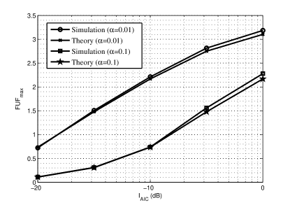
Figure 2: Comparison of maximum FUF of feedback efficient adaptive mode selection based on numerical simulation and theoretical deduction.

TABLE I: The optimal transmission mode and feedback bits with different path losses

		$I_{\textrm{AIC}}$	-20dB	-15dB	-10dB	-5dB	0dB
		$B_{\textrm{opt}}$	0	4	1	0	0
$\alpha=0.01$	OA	$M_{\textrm{opt}}$	4	2	2	2	2
		$B_{\textrm{opt}}$	0	4	1	0	0
	SA	$M_{\textrm{opt}}$	4	2	2	2	2
		$B_{\textrm{opt}}$	0	0	0	4	1
$\alpha=0.1$	OA	$M_{\textrm{opt}}$	4	4	4	2	2
		$B_{\textrm{opt}}$	0	0	0	4	1
	SA	$M_{\textrm{opt}}$	4	4	4	2	2

Secondly, we show the performance gain from cooperative feedback by comparing the performance of the proposed scheme and a fixed scheme with $\alpha=0.01$ and $C=2$. As the name implies, the fixed scheme sets $M=N_{t}=5$ and $B=0$, namely without cooperation from primary network. Note that the fixed scheme has a larger multiplexing gain, since there is no need of extra spatial degree of freedom for mitigating the interference to primary receiver. In spite of this, the proposed scheme performs better than the fixed scheme obviously in the whole range of $I_{\textrm{AIC}}$. As seen in Fig.3, as $I_{\textrm{AIC}}$ relaxes, the performance gain becomes larger and larger. It is worth pointing out that from the perspective of average transmission rate, the proposed scheme has more gains, since FUF${}_{\textrm{max}}$ takes into consideration of feedback cost. Therefore, the proposed scheme can effectively improve the performance.

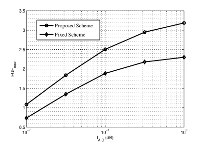
Figure 3: Comparison of maximum FUF of proposed scheme and fixed scheme.

Next, we investigate the impact of feedback amount of cognitive user on the optimal mode selection, feedback bits and FUF${}_{\textrm{max}}$. In this case, we fix $\alpha=0.01$ and $\mu=0.1$. Intuitively, the larger $C$ is conducive to improve FUF${}_{\textrm{max}}$, since more accurate CSI can further decrease the inter-user interference. As seen in Fig.4, at $I_{\textrm{AIC}}=-10$dB, FUF${}_{\textrm{max}}$ for $C=6$ has a performance gain of about $1.0$dB over that for $C=2$, and the gain increases with a lower AIC requirement. In addition, as analyzed in Section IV, the impacts of a small $\alpha$ and a large $C$ are contrary, so that $B_{\textrm{opt}}$ is unequal to 0 when $C=6$ and $I_{\textrm{AIC}}\leq-10$dB, as shown in Tab.II. However, as $I_{\textrm{AIC}}$ increases, $B_{\textrm{opt}}$ becomes small gradually, and $B_{\textrm{opt}}=0$ when $I_{\textrm{AIC}}=0$dB.

Figure 4: Comparison of maximum FUF of feedback efficient adaptive mode selection with different feedback amount.

TABLE II: The optimal transmission mode and feedback bits with different feedback amount

		$I_{\textrm{AIC}}$	-20dB	-15dB	-10dB	-5dB	0dB
		$B_{\textrm{opt}}$	0	4	1	0	0
$C=2$	OA	$M_{\textrm{opt}}$	4	2	2	2	2
		$B_{\textrm{opt}}$	0	4	1	0	0
	SA	$M_{\textrm{opt}}$	4	2	2	2	2
		$B_{\textrm{opt}}$	4	4	4	0	0
$C=4$	OA	$M_{\textrm{opt}}$	4	2	2	2	2
		$B_{\textrm{opt}}$	4	4	4	0	0
	SA	$M_{\textrm{opt}}$	4	2	2	2	2
		$B_{\textrm{opt}}$	4	4	4	1	0
$C=6$	OA	$M_{\textrm{opt}}$	4	4	2	2	2
		$B_{\textrm{opt}}$	4	4	4	1	0
	SA	$M_{\textrm{opt}}$	4	4	2	2	2

Then, we compares the FUF${}_{\textrm{max}}$s of feedback efficient adaptive mode selection with different pricing factors. In this scenario, we fix $C=5$ and $\alpha=0.01$. As seen in Fig.5, $\mu$ has a relatively slight impact on the FUF${}_{\textrm{max}}$. Especially when $I_{\textrm{AIC}}$ becomes less loose, such as $I_{\textrm{AIC}}>-5$dB, FUF${}_{\textrm{max}}$ is hardly changed as the pricing factor $\mu$ increases. This is because cognitive BS purchases less feedback bits and transmission mode keeps constant. Once pricing factor $\mu$ rises, as shown in Tab.III, both available transmit power and feedback cost descend simultaneously, and thus FUF${}_{\textrm{max}}$ is not so unsensitive to $\mu$. Additionally, for a given $\mu$, with the increase of AIC, the required $B_{\textrm{opt}}$ decreases gradually, and reduces to 0 finally when $I_{\textrm{AIC}}$ is large enough, and this is consistent of the asymptotic analysis result. With the increase of $\mu$, $B_{\textrm{opt}}$ is equal to 0 even with a strict AIC. Meanwhile, the strict AIC leads to full multiplexing, namely $M_{\textrm{opt}}=N_{t}-1$, because the cognitive network is interference-limited under such a condition. These conclusions are helpful to determine the extent of cooperation in practical networks.

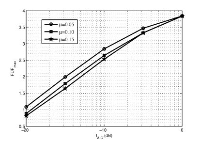
Figure 5: Comparison of maximum FUF of feedback efficient adaptive mode selection with different pricing factors.

TABLE III: The optimal transmission mode and feedback bits with different pricing factors

		$I_{\textrm{AIC}}$	-20dB	-15dB	-10dB	-5dB	0dB
		$B_{\textrm{opt}}$	4	4	4	4	1
$\mu=0.05$	OA	$M_{\textrm{opt}}$	4	4	2	2	2
		$B_{\textrm{opt}}$	4	4	4	4	1
	SA	$M_{\textrm{opt}}$	4	4	2	2	2
		$B_{\textrm{opt}}$	4	4	4	0	0
$\mu=0.10$	OA	$M_{\textrm{opt}}$	4	4	2	2	2
		$B_{\textrm{opt}}$	4	4	4	0	0
	SA	$M_{\textrm{opt}}$	4	4	2	2	2
		$B_{\textrm{opt}}$	0	0	0	0	0
$\mu=0.15$	OA	$M_{\textrm{opt}}$	4	4	2	2	2
		$B_{\textrm{opt}}$	0	0	0	0	0
	SA	$M_{\textrm{opt}}$	4	4	2	2	2

Finally, we consider the scenario in presence of feedback delay during conveying interference CSI, and the delay for feedback link of cognitive network can be neglected due to the relatively short access distance. Similarly, we fix $C=5$ and $\alpha=0.01$ in this scenario. Surprisingly, it is seen from Fig.6 that FUF${}_{\textrm{max}}$ is quite unsensitive to feedback delay. For $\mu=0.1$, even with large feedback delay, such as $\rho=0.5$, FUF${}_{\textrm{max}}$ coincides with that of ideal case, namely $\rho=1$. Furthermore, FUF${}_{\textrm{max}}$ for $\rho=0.5$ may be slightly better than that of $\rho=1$ under some conditions, such as a loose AIC, which reconfirms to the theoretical claim earlier. Meanwhile, Tab.IV shows that feedback delay will not change the optimal transmission mode when $\mu=0.1$. If $\mu$ is sufficient small, such as $\mu=0.01$, as many feedback bits as possible is used due to such a low price. Under this condition, the case of $\rho=0.5$ has a performance loss, because it can not compensate the loss caused by decreasing feedback bits. However, in practical networks, cognitive networks is impossible to obtain the cooperation on such a low cost, so the proposed feedback efficient adaptive mode selection is robust under various scenarios.

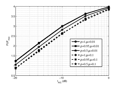
Figure 6: Comparison of maximum FUF of feedback efficient adaptive mode selection with different correlation coefficients.

TABLE IV: The optimal transmission mode and feedback bits with different correlation coefficients

		$I_{\textrm{AIC}}$	-20dB	-15dB	-10dB	-5dB	0dB
		$B_{\textrm{opt}}$	4	4	4	4	4
$\rho=1$	OA	$M_{\textrm{opt}}$	4	4	2	2	2
$\mu=0.01$		$B_{\textrm{opt}}$	4	4	4	4	4
	SA	$M_{\textrm{opt}}$	4	4	2	2	2
		$B_{\textrm{opt}}$	4	4	4	4	4
$\rho=0.95$	OA	$M_{\textrm{opt}}$	4	4	2	2	2
$\mu=0.01$		$B_{\textrm{opt}}$	4	4	4	4	4
	SA	$M_{\textrm{opt}}$	4	4	2	2	2
		$B_{\textrm{opt}}$	4	4	4	4	4
$\rho=0.5$	OA	$M_{\textrm{opt}}$	4	4	2	2	2
$\mu=0.01$		$B_{\textrm{opt}}$	4	4	4	4	4
	SA	$M_{\textrm{opt}}$	4	4	2	2	2
		$B_{\textrm{opt}}$	4	4	4	0	0
$\rho=1$	OA	$M_{\textrm{opt}}$	4	4	2	2	2
$\mu=0.1$		$B_{\textrm{opt}}$	4	4	4	0	0
	SA	$M_{\textrm{opt}}$	4	4	2	2	2
		$B_{\textrm{opt}}$	4	4	4	0	0
$\rho=0.95$	OA	$M_{\textrm{opt}}$	4	4	2	2	2
$\mu=0.1$		$B_{\textrm{opt}}$	4	4	4	0	0
	SA	$M_{\textrm{opt}}$	4	4	2	2	2
		$B_{\textrm{opt}}$	0	0	0	0	0
$\rho=0.5$	OA	$M_{\textrm{opt}}$	4	4	2	2	2
$\mu=0.1$		$B_{\textrm{opt}}$	0	0	0	0	0
	SA	$M_{\textrm{opt}}$	4	4	2	2	2

VI Conclusion

A major contribution of this paper is to propose a limited cooperation between primary and cognitive networks, so as to take advantage of the benefit of multiantenna at cognitive BS through ZFBF. In order to utilize the feedback information from primary receiver effectively, this paper further proposes to maximize the feedback utility function while satisfying the interference constraint by optimizing transmission mode and feedback bits. With the goal of enhancing the usability of the present adaptive mode selection scheme in practical networks, we investigate the effect of feedback delay on feedback utility function and derive the corresponding optimal transmission scheme. In addition, we present some low-complexity schemes through asymptotic characteristics analysis.

References

- [1] FCC, “Spectrum policy taks force report,” ET Docket 02-155, Nov. 2002.
- [2] I. J. Mitola, “Software radio: survay, critical evaluation and future direction,” IEEE Aerosp. Elecron. Syst. Mag., vol. 8, pp. 25-31, Apr. 1993.
- [3] B. Wang, and K. J. R. Liu, “Advances in cognitive radio networks: a survey,” IEEE J. Sel. Topics Signal Process., vol. 5, no. 1, pp. 5-23, Feb. 2011.
- [4] S. Haykin, D. J. Thomson, and J. H. Reed, “Spectrum sensing for cognitive radio,” Proceedings of the IEEE, vol. 97, no. 5, pp. 849-877, May 2009.
- [5] S. Makeki, and G. Leus, “Censored truncated sequential spectrum sensing cog cognitive radio networks,” IEEE J. Sel. Areas Commun., vol. 31, no. 3, pp. 364-378, Mar. 2013.
- [6] R. Deng, J. Chen, C. Yuen, P. Cheng, Y. Sun, “Energy-efficient cooperative spectrum sensing by optimal scheduling in sensor-aided cognitive radio networks,” IEEE Trans. Veh. Tech., vol. 61, no. 2, pp. 716-725, Feb. 2012.
- [7] Y. Chen, G. Yu, Z. Zhang, H. Chen, and P. Qiu, “On cognitive radio networks with opportunistic power control strategies in fading channels,” IEEE Trans. Wireless Commun., vol. 7, no. 7, pp. 2752-2761, Jul. 2008.
- [8] V. D. Papoutsis and A. P. Stamouli, “Chunk-based resource allocation in multicast MISO-OFDMA with average BER constraint,” IEEE Commun. Lett., vol. 17, no. 2, pp. 317-320, Feb. 2013.
- [9] V. D. Papoutsis and S. A. Kotsopoulos, “Chunk-based resource allocation in distributed MISO-OFDMA systems with fairness guarantee,” IEEE Commun. Lett., vol. 15, no. 4, pp. 377-379, Apr. 2011.
- [10] F. Gao, R. Zhang, Y-C. Liang, X. Wang, “Design and learning-based MIMO cognitive radio systems,” IEEE Trans. Veh. Tech., vol. 59, no. 4, pp. 1707-1720, May 2010.
- [11] X. Chen, and H-H. Chen, “Interference-aware resource control in multi-antenna cognitive ad hoc networks with heterogeneous delay constraints,” IEEE Commun. Lett., vol. 17, no. 6, pp. 1184-1187, Apr. 2013.
- [12] X. Zeng, Q. Li, Q. Zhang, and J. Qin, “Joint beamforming and antenna subarray formation for MIMO cognitive radio,” IEEE Signal Process. Lett., vol. 20, no. 5, pp. 479-482, May 2013.
- [13] J. Noh, and S. Oh, “Beamforming in a multi-user cognitive radio system with partial channel state information,” IEEE Trans. Wireless Commun., vol. 12, no. 2, pp. 616-625, Feb. 2013.
- [14] R. Zhang, and Y-C. Liang, “Exploiting multi-antennas for opportunistic spectrum sharing in cognitive radio networks,” IEEE J. Sel. Topics Signal Process., vol. 2, no. 1, pp. 88-102, Feb. 2008.
- [15] X. Chen, and C. Yuen, “Efficient resource allocation in rateless coded MU-MIMO cognitive radio network with QoS provisioning and limited feedback,” IEEE Trans. Veh. Tech., vol. 62, no. 1, pp. 395-399, Jan. 2013.
- [16] L. Zhang, Y-C. Liang, Y. Xin, and H. Poor, “Robust cognitive beamforming with partial channel state information,” IEEE Trans. Wireless Commun., vol. 8, no. 8, pp. 4143-4152, Aug. 2009.
- [17] K. Hamdi, W. Zhang, K. B. Letaief, “Joint beamforming and scheduling in cognitive radio network,” in Proc. IEEE Globecom, pp. 2977-2981, Nov. 2007.
- [18] R. Zhang, and Y-C. Liang, “Investigation on multiuser diversity in spectrum sharing based cognitive radio networks,” IEEE Commun. Lett., vol. 14, no. 2, pp. 133-135, Feb. 2010.
- [19] M. H. Islam, Y-C. Liang, and A. T. Hoang, “Joint power control and beamforming for cognitive radio networks,” IEEE Trans. Wireless Commun., vol. 7, no. 7, pp. 2415-249, Jul. 2008.
- [20] D. J. Love, R. W. Heath Jr., V. K. N. Lau, D. Gesbert, B. D. Rao, and M. Andrews, “An overview of limited feedback in wireless communication systems,” IEEE J. Sel. Areas Commun., vol. 26, no. 8, pp. 1341-1365, Oct. 2008.
- [21] H. Yang, J. Chun, and Y. Choi, “Codebook-based lattice-reduction-aided precoding for limited-feedback coded MIMO systems,” IEEE Trans. Commun., vol. 60, no. 2, pp. 510-524, Feb. 2012.
- [22] K. Huang, and R. Zhang, “Cooperative feedback for multiantenna cognitive radio networks,” IEEE Trans. Signal Process., vol. 59, no. 2, pp. 747-758, Feb. 2011.
- [23] S. Ganesan, M. Sellathurai, and T. Ratnarajah, “Opportunistic interference projection in cognitive MIMO radio with multiuser diversity,” IEEE New Frontiers in Dynamic Spectrum, pp. 1-6, Apr. 2010.
- [24] L. Liu, R. Chen, S. Geirhofer, K. Sayana, Z. Shi, and Y. Zhou, “Downlink MIMO in LTE-advanced: SU-MIMO vs. MU-MIMO,” IEEE Commun. Mag., vol. 50, no. 2, pp. 140-147, Feb. 2012.
- [25] X. Chen, Z. Zhang, S. Chen, and C. Wang, “Adaptive mode selection for multiuser MIMO downlink employing rateless codes with QoS provioning,” IEEE Trans. Wireless Commun., vol. 11, no. 2, pp. 790-799, Feb. 2012.
- [26] J. Zhang, M. Kountouris, J. G. Andrews, and R. W. Heath Jr., “Multi-mode transmission for the MIMO broadcast channel with imperfect channel state information,” IEEE Trans. Commun., vol. 59, no. 3, pp. 803-814, Mar. 2011.
- [27] R. Zhang, “On peak versus average intererence power constraints for protecting primary users in cognitive radio networks,” IEEE Trans. Wireless Commun., vol. 8, no. 4, pp. 2112-2120, Apr. 2009.
- [28] C-X. Wang, X. Hong, H-H. Chen, and J. Thompson, “On capacity of cognitive radio networks with average interference power constraints,” IEEE Trans. Wireless Commun., vol. 8, no. 4, pp. 1620-1625, Apr. 2009.
- [29] X. Kang, R. Zhang, and M. Motani, “Price-based resource allocation for spectrum-sharing femtocell networks: a stackelberg game,” IEEE J. Sel. Areas Commun., vol. 30, no. 3, pp. 538-549, Apr. 2012.
- [30] N. Jindal, “MIMO Broadcast channels with finite-rate feedback,” IEEE Trans. Inf. Theory, vol. 52, no. 11, pp. 5045-5060, Nov. 2006.
- [31] K. K. Mukkavilli, A. Sabharwal, E. Erkip, and B. Aazhang, “On beamforming with finite rate feedback in multiple-antenna systems,” IEEE Trans. Inf. Theory, vol. 49, no. 10, pp. 2562-2579, Oct. 2003.
- [32] Y. Isukapalli, and B. D. Rao, “Finite rate feedback for spatially and temporally correlated MISO channels in the presence of estimation errors and feedback delay,” in Proc. IEEE GLOBECOM, pp. 2791-2795, Nov. 2007.