Radiative symmetry breaking at the Fermi scale
and
flat potential at the Planck scale

Abstract

We investigate a possibility of the “flatland scenario”, in which the electroweak gauge symmetry is radiatively broken via the Coleman-Weinberg mechanism starting from a completely flat Higgs potential at the Planck scale. We show that the flatland scenario is realizable only when an inequality $K<1$ among the coefficients of the $\beta$-functions is satisfied. We show several models satisfying the condition.

Introduction.— The Brout-Englert-Higgs (BEH) mechanism in the context of the Standard Model (SM) is the source of the electroweak symmetry breaking (EWSB) and predicts appearance of the Higgs boson BEH-mechanism . Recently the LHC experiment announced the discovery of a new particle like the Higgs boson in the SM and its mass is now determined to be $m_{H}=125$–$126$ GeV Higgs-discover . This mass causes the so-called stability problem of the SM vacuum. Compared with the value of the condensation $v=246$ GeV, the mass is relatively small and the Higgs potential seems to be shallow. The shallowness indicates instability of the potential against the radiative corrections, and indeed, if we calculate the running quartic coupling of the Higgs boson $\lambda_{H}(\mu)$ where $\mu$ is the renormalization scale, it tends to vanish at a very high energy scale stability . Within the uncertainties of the top quark mass and the strong gauge coupling, the running Higgs coupling seems to vanish asymptotically $\lambda_{H}(\mu)\rightarrow 0$ near the Planck scale $\mu\rightarrow M_{Pl}$.

Another important hint for the origin of the Higgs potential comes from the naturalness problem. The Higgs mass receives large radiative corrections by, if exist, heavy particles coupled to the Higgs boson. The supersymmetry in the TeV scale gives a beautiful solution to the naturalness problem, but the LHC and other precision experiments have strong constraints on their masses. Also, the Technicolor scenario is faced with the difficulties of the $S$-parameter and the smallness of the Higgs mass. Recently alternative solutions to the naturalness problem are widely discussed naturalness . Suppose that the UV completion theory (which may be beyond the ordinary field theories like the string theory) is connected with the SM sector in a way that the SM has no dimensionful parameters. Then if no large intermediate mass scales exist between the SM and the UV completion theory, no large logarithmic corrections violating the multiplicative renormalization of the Higgs mass term are generated and the SM becomes free from the naturalness problem. Such a model based on the idea is called a classically conformal model with no intermediate scales ccm ; Iso:2009ss .

Motivated by the stability of the vacuum and the naturalness problem, we explore a possibility Iso:2012jn ; Chun:2013soa that the EW symmetry is radiatively broken in the infrared (IR) region via the Coleman-Weinberg mechanism (CWM) CW starting from a flat scalar potential in the ultraviolet (UV) region. We call it a ”flatland scenario”. It is nontrivial to construct such a model because the scalar quartic coupling must be tuned to become very small both in the IR and the UV regions. It is well known that the CWM does not work within the SM because of the large top Yukawa coupling. Thus we need to extend the SM by introducing an additional sector in which the dynamical mass generation occurs. In this letter, we show that a certain inequality $K<1$ must be satisfied among the coefficients of the $\beta$ functions in order to realize the flatland scenario.

A necessary condition for the flatland.— We first consider a system of a complex scalar field $\Phi$ charged under the Abelian gauge field. We further introduce a charged fermion $\psi$ with a (Majorana) Yukawa coupling $y$ to the scalar field. The gauge coupling is denoted by $g$ and $\lambda$ is the quartic coupling of the scalar field. The RGE’s can be written in terms of model-dependent positive constants $a,b,c,d,f$ as

$$\beta_{g} \equiv \mu\frac{\partial}{\partial\mu}g=\frac{a}{16\pi^{2}}g^{3},$$ (1)

$$\beta_{y} \equiv \mu\frac{\partial}{\partial\mu}y=\frac{y}{16\pi^{2}}\bigg{[}\,by^{2}-cg^{2}\,\bigg{]},$$ (2)

$$\beta_{\lambda} \equiv \mu\frac{\partial}{\partial\mu}\lambda=\frac{1}{16\pi^{2}}\bigg{[}\,-dy^{4}+fg^{4}+\cdots\,\bigg{]}\,.$$ (3)

The dots in $\beta_{\lambda}$ include terms $\lambda^{2}$, $\lambda g^{2}$, etc. They are irrelevant in the following discussions because the quartic coupling $\lambda$ becomes very small both in the IR region where the CWM occurs and in the UV region where we impose $\lambda(\Lambda)=0$ at a UV scale $\Lambda$. Introducing $t=(\ln\mu/M)/16\pi^{2}$ ($M$ is an IR scale) and the new variable $r=y/g$, we can rewrite eqs. (2),(3) into

$$\dot{r}=brg^{2}(r^{2}-r_{c}^{2}),\ \ \dot{\lambda}=dg^{4}(r_{0}^{4}-r^{4}),$$ (4)

where the dot denotes $t$-derivative and $r_{c},r_{0}$ are the zeros of the $\beta$-functions of $r=y/g$ and $\lambda$ respectively;

$$r_{c}=\sqrt{\frac{a+c}{b}},\ \ r_{0}=\left(\frac{f}{d}\right)^{1/4}.$$ (5)

From the first equation of (4), we can see that $r=r_{c}$ is an IR fixed point Pendleton:1980as for the ratio $r$, i.e., if $r>r_{c}$ (or $r<r_{c})$, $r(t)$ is an increasing (decreasing) function of $t$.

Now let us study the condition for the flatland scenario, namely the condition that the gauge symmetry is spontaneously broken with a vacuum expectation value $\langle\Phi\rangle=M/\sqrt{2}$ via the CWM in a model with a vanishing quartic coupling at the UV scale, $\lambda(t_{UV})=0$. A typical behavior of the running quartic coupling $\lambda_{\Phi}$ is given in figure 1. This figure shows that in the IR region $t\sim 0$, the $\beta$-function of $\lambda$ must be positive $\beta_{\lambda}(t=0)>0$ while being negative $\beta_{\lambda}(t_{UV})<0$ in the UV. Hence $r(t)$ must satisfy the inequalities $r(t=0)<r_{0}<r(t_{UV}).$ Then, since $r(t)$ is an increasing function of $t$, it must be larger than $r_{c}$;

$$r_{c}<r(t=0)<r_{0}<r(t_{UV}).$$ (6)

Hence we obtain a necessary condition among the coefficients of the $\beta$-functions for the flatland scenario;

$$K=\left(\frac{r_{c}}{r_{0}}\right)^{2}=\frac{a+c}{b}\sqrt{\frac{d}{f}}<1.$$ (7)

Unless the inequality is satisfied, the radiative symmetry breaking, namely the CWM, does not occur starting from the flat potential at the UV scale.

It is furthermore required that the ratio $r(0)=y(0)/g(0)$ at the IR scale is tuned to lie in-between $r_{c}$ and $r_{0}$. This fact is followed by the smallness of the scalar boson mass in a model with $K$ close to 1, $K\lesssim 1.$ In the CWM, the scalar boson acquires its mass proportional to the $\beta$ function (see, e.g., eq.(4) in the first paper of Iso:2009ss ),

$$m_{\phi}^{2}=\beta_{\lambda}(0)M^{2}=\frac{M^{2}}{16\pi^{2}}\left(-dy^{4}(M)+fg^{4}(M)\right)>0.$$ (8)

Hence, if $K\lesssim 1$, $r_{c}\sim r_{0}$ and $r(0)$ is also very close to $r_{0}$. Thus $\beta_{\lambda}(0)\sim 0$ and the scalar mass of eq.(8) becomes tiny. We will see such a situation explicitly below.

Let us now evaluate the ratio $K$ for the $B-L$ (baryon minus lepton number) models with the Majorana Yukawa interactions between the SM singlet complex scalar field $\Phi$ and the right-handed neutrinos $\nu_{Ri}$,

$${\cal L}_{M}=-Y_{M}^{ij}\overline{\nu_{Ri}^{c}}\,\nu_{Rj}\Phi+\mbox{(h.c.)}\,.$$ (9)

The coefficients of the RGE’s read Iso:2009ss ; Basso:2010jm ; Iso:2012jn

$$a = \frac{32}{9}N_{g}+\frac{4}{3}N_{\Phi},\quad b=4+2N_{\nu},$$

$$c = 6,\quad d=16N_{\nu},\quad f=96,$$ (10)

where $N_{g}$ is the number of generations coupled to the $U(1)_{B-L}$ gauge field and $N_{\Phi}\;(=1)$ is the number of $\Phi$. $N_{\nu}$ stands for the number of the right handed neutrinos having relevant Majorana couplings. For simplicity, we take $Y_{M}^{ij}=\mathrm{diag}(y_{M},\cdots,y_{M},0,\cdots,0)$ and $\mathrm{tr}[(Y_{M}^{ij})^{2}]=N_{\nu}y_{M}^{2}$ etc. We denote these models by $(N_{g},N_{\Phi},N_{\nu})$.

The ratios $K$ for various $B-L$ models are listed in the Table 1. In the $(3,1,N_{\nu})$ models, K is always larger than $1$. Hence the flatland scenario does not occur in the models with $N_{g}=3$.

In order to satisfy the condition (7), we will consider two possibilities, (1) decreasing $a$, or (2) increasing $b$ (or $N_{\nu}$). The first possibility is realized for smaller $N_{g}$. From the Table 1, we see that $K<1$ for $N_{g}=1,2$ and $N_{\nu}=1$. These are the candidates of the flatland scenario. The second possibility is to introduce SM and $B-L$ singlet fermions so that $N_{\nu}$ is larger than three.

$$\begin{array}[]{c|l}\hline\cr N_{g}=3&\begin{array}[]{c|l}N_{\nu}=1&K=\sqrt{3/2}\simeq 1.22\\ N_{\nu}=2&K=3\sqrt{3}/4\simeq 1.30\\ N_{\nu}=3&K=9\sqrt{2}/10\simeq 1.27\\ \end{array}\\ \hline\cr N_{g}=2&\begin{array}[]{c|l}N_{\nu}=1&K=65\sqrt{6}/162\simeq 0.98\\ N_{\nu}=2&K=65\sqrt{3}/108\simeq 1.04\\ \end{array}\\ \hline\cr N_{g}=1&\begin{array}[]{c|l}N_{\nu}=1&K=49\sqrt{6}/162\simeq 0.74\\ \end{array}\\ \hline\cr\end{array}$$

Table 1: Values of $K$ for various $B-L$ models $(N_{g},N_{\Phi},N_{\nu})$. We fixed to $N_{\Phi}=1$, which minimizes $K$ with respect to $N_{\Phi}$. The flatland scenario is possible only when $K<1$.

Flatland scenario.— We investigate more detailed analysis of the RGE’s in the flatland scenario and show how the EWSB is triggered by the $B-L$ symmetry breaking. The Lagrangian of the $B-L$ model is

$${\cal L}={\cal L}_{\rm SM}+{\cal L}_{\rm kin}+{\cal L}_{M}-V,$$ (11)

where ${\cal L}_{\rm SM}$ represents the SM part, ${\cal L}_{\rm kin}$ is the kinetic terms of $\nu_{R}$, $\Phi$ and the $B-L$ gauge field $B^{\prime}_{\mu}$. We fix $N_{\Phi}=1$. The potential for the Higgs doublet $H$ and the SM singlet $\Phi$ is given by $V$,

$$V=\lambda_{H}|H|^{4}+\lambda_{\Phi}|\Phi|^{4}+\lambda_{\mathrm{mix}}|H|^{2}|\Phi|^{2}.$$ (12)

We assumed the classical conformality, i.e., the mass squared terms are absent. In the basis where the two $U(1)$ gauge kinetic terms are diagonal, the covariant derivative is written as

$$D_{\mu} = \partial_{\mu}-ig_{3}\frac{\lambda^{a}}{2}G_{\mu}^{a}-ig_{2}\frac{\tau^{i}}{2}W_{\mu}^{i}$$ (13)

$$-iY(g_{Y}B_{\mu}+g_{\mathrm{mix}}B^{\prime}_{\mu})-ig_{B-L\rule{0.0pt}{7.0pt}}Y_{B-L}B^{\prime}_{\mu},$$

where $Y$ and $Y_{B-L}$ denote the hypercharge and the $B-L$ charge, respectively. The gauge couplings of $SU(3)_{c}$, $SU(2)_{W}$, $U(1)_{Y}$ and $U(1)_{B-L}$ are $g_{3}$, $g_{2}$, $g_{Y}$ and $g_{B-L\rule{0.0pt}{7.0pt}}$, respectively. In general, the $U(1)$ gauge mixing $g_{\mathrm{mix}}$ appears owing to the loop corrections of the fermions having both charges of $U(1)_{Y}$ and $U(1)_{B-L}$, even if we impose $g_{\mathrm{mix}}=0$ at some scale.

For appropriate parameters investigated below, the CWM occurs in the $B-L$ sector of $\Phi$ Iso:2009ss ; Iso:2012jn . Then the EWSB takes place if the $H$–$\Phi$ mixing term $\lambda_{\mathrm{mix}}|H|^{2}|\Phi|^{2}$ is negative;

$$v_{H}^{2}=\frac{-\lambda_{\mathrm{mix}}}{2\lambda_{H}}\,v_{\Phi}^{2},$$ (14)

where $\langle H\rangle=(0,\;v_{H}/\sqrt{2})^{T}$ and $\langle\Phi\rangle=v_{\Phi}/\sqrt{2}$. The Higgs mass $m_{h}$ is approximately given by $m_{h}^{2}=2\lambda_{H}v_{H}^{2}$, because the mixing between $H$ and $\Phi$ is tiny. In Iso:2012jn , we have shown that such a small and negative scalar mixing is radiatively generated through the gauge kinetic mixing of $U(1)_{B-L}$ and $U(1)_{Y}$.

In order to realize the flatland scenario, we impose vanishing of the scalar potential at a UV scale $\Lambda$,

$$\lambda_{H}(\Lambda)=0,\quad\lambda_{\Phi}(\Lambda)=0,\quad\lambda_{\mathrm{mix}}(\Lambda)=0.$$ (15)

We also set $g_{\mathrm{mix}}(\Lambda)=0$ by constructing a model with no $U(1)$ kinetic mixing at the high energy scale $\Lambda$. The gauge mixing $g_{\mathrm{mix}}\neq 0$ between $Z$ and $Z^{\prime}$ is generated in the EW scale through the RG effects. It is potentially dangerous, but we find that the deviation of the $\rho$ parameter from unity is tiny, at most $\delta\rho_{0}\sim{\cal O}(10^{-5})$ HIO . The remaining parameters are $g_{B-L\rule{0.0pt}{7.0pt}}$ and $y_{M}$, which correspond to the masses of $Z^{\prime}$ and $\nu_{R}$,

$$M_{Z^{\prime}}\simeq 2g_{B-L\rule{0.0pt}{7.0pt}}v_{\Phi},\quad M_{\nu_{R}}\simeq\sqrt{2}\,y_{M}v_{\Phi}.$$ (16)

Starting from the flat potential (15) at the UV scale, running couplings are obtained dynamically by solving the RGE’s, and the value of $v_{H}$ in Eq. (14) is predicted in terms of them. The RG flows are controlled by the gauge coupling $g_{B-L}$ and the Majorana Yukawa coupling $y_{M}$ at $\Lambda$ besides the SM parameters. Given these two parameters at $\Lambda$, the symmetry breaking scales of $\Phi$ and $H$ are determined. In order to set $v_{H}=246$ GeV, we must adjust one of the two parameters in accordance with the other. Hence there is only one free parameter in the model. In particular, the CW relation

$$\frac{m_{\phi}^{2}}{M_{Z^{\prime}}^{2}}+N_{\nu}\frac{g^{2}_{B-L\rule{0.0pt}{6.0pt}}}{\pi^{2}}\frac{M_{\nu_{R}}^{4}}{M_{Z^{\prime}}^{4}}\simeq\frac{3g^{2}_{B-L\rule{0.0pt}{6.0pt}}}{2\pi^{2}}$$ (17)

must hold where we rewrote the equation (8) in terms of the physical quantities.

Numerical analysis.— We numerically solve the RGE’s of the $(2,1,1)$ and $(1,1,1)$ models. In the following analysis, we take the UV scale at $\Lambda=1/\sqrt{8\pi G}=2.435\times 10^{18}$ GeV. Also, we fix the Higgs mass, $m_{h}=126.8$ GeV and the $\overline{MS}$ mass of the top quark $\overline{m_{t}}=160.4$ GeV so as to realize $\lambda_{H}(\Lambda)=0$ .

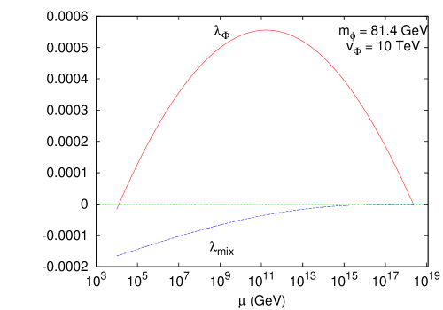
Figure 1: The RG flows of $\lambda_{\Phi}$ and $\lambda_{\mathrm{mix}}$ in $(2,1,1)$ model. $v_{\Phi}=10$ TeV, $m_{\phi}=81.4$ GeV and $y_{M}(v_{\Phi})=0.378$. $K$ is close to $1$ and the quartic coupling $\lambda_{\Phi}$ is small. Accordingly, the scalar mass becomes very light compared with $v_{\Phi}$.

We first investigate the $(2,1,1)$ model. Since $K=0.98$, the necessary condition for the flatland scenario is barely satisfied, suggesting that the SM singlet scalar mass $m_{\phi}$ is very light compared to the gauge boson mass $M_{Z^{\prime}}$. If we take, for example, $v_{\Phi}=10$ TeV, the other parameters are numerically determined to be $m_{\phi}=81.4$ GeV, $y_{M}(v_{\Phi})=0.378$ and $M_{Z^{\prime}}=4.87$ TeV. The scalar mass is actually light. The RG flows of $\lambda_{\Phi}$ and $\lambda_{\mathrm{mix}}$ are depicted in Fig. 1. The very small quartic coupling $\lambda_{\Phi}$ corresponds to the lightness of $m_{\phi}$. Fig. 2 shows relations between $m_{\phi},M_{\nu_{R}}$ and $M_{Z^{\prime}}$. When $m_{\phi}^{2}\ll g^{2}_{B-L\rule{0.0pt}{6.0pt}}M_{Z^{\prime}}^{2}$, we get approximately $M_{\nu_{R}}\sim\sqrt[4]{3/(2N_{\nu})}\,M_{Z^{\prime}}$ from the CW relation (17). We also comment that $K=1$ is possible if we choose appropriately the second largest $Y_{M}^{ij}$. Then the scalar potential becomes flat in all energy scales, and $\Phi$ becomes massless.

Figure 2: $M_{Z^{\prime}}$ vs $M_{\nu_{R}}$and $m_{\phi}$ for the $(2,1,1)$ model. $M_{\nu_{R}}$ is almost proportional to $M_{Z^{\prime}}$.

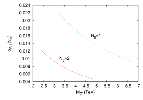
Figure 3: $M_{Z^{\prime}}$ vs $\alpha_{B-L}(v_{\Phi})$ for the $(2,1,1)$ and $(1,1,1)$ models.

For the $(1,1,1)$ model, we obtain similar results, but not repeated here. Figures 3 shows the relation between $M_{Z^{\prime}}$ and $\alpha_{B-L}$ for the $(2,1,1)$ and $(1,1,1)$ models. The gauge coupling is relatively larger for a fixed $M_{Z^{\prime}}$ than the prediction of $(3,1,1)$ model studied in Iso:2012jn .

In the $(2,1,1)$ and $(1,1,1)$ models, the off diagonal terms in the SM yukawa couplings are not written in dimension four operators. For this purpose, we may introduce an additional scalar field $S$ with a fractional $B-L$ charge such as

$${\cal L}_{\rm off}=-Y_{\nu}^{(13)}\overline{\ell^{(1)}_{L}}\tilde{H}\nu_{R}^{(3)}\left(\frac{S}{\Lambda}\right)^{k}+\cdots\,.$$ (18)

A simple model contains a scalar $S$ with $Q=1/3$ $B-L$ charge. In this case $K$ becomes $K=0.985$, and the flatland scenario is still possible. More generally, including $n$ additional scalars with $B-L$ charge $Q$ into the $(2,1,1)$ model, the ratio $K$ is modified to be $K=\sqrt{6}/108(130/3+nQ^{2})$.

The introduction of the scale $\Lambda$ in (18) is not favourable from the standpoint of the classical conformality. It can be evaded if we regard the $N_{g}=1,2$ sector as extra (or “hidden”) generations like in Ref. Lee:2012xn . In this case, the higher-dimensional terms are not required and the model can be compatible with the classical conformality of the SM sector.

Another possibility is to introduce extra Higgs doublets with the $B-L$ charges. Furthermore, $U(1)^{\prime}$ models are not restricted only to the $B-L$ one Langacker:2008yv . An example of such generalisations was investigated in the corrigendum to Chun:2013soa .

The second type of possibility of the flatland scenario is to introduce $N_{\nu}$ singlet fermions $\psi_{sj}$ with a coupling $\overline{\nu^{c}_{Ri}}\psi_{sj}\Phi$, where the $B-L$ charge of $\Phi$ should be changed appropriately, and a Majorana mass term for them instead of the Majorana Yukawa couplings. In such a model, the condition $K<1$ is satisfied for $N_{\nu}\sim{\cal O}(100)$.

Summary.— The origin of the Higgs potential is one of the unsolved issues in particle physics. We explore possibilities that the EWSB occurs starting from a completely flat potential at a UV energy scale. The scenario, which we call the flatland scenario, is possible only when the system satisfies an inequality $K<1$ of eq.(7). This is the main result of the paper. The condition gives a strong constraint when we construct a model of the radiative EWSB with a flat potential at the Planck scale flat . We schematically showed some models satisfying the condition. More detailed analysis are investigated in a separate paper HIO .

References

- (1) F. Englert and R. Brout, Phys. Rev. Lett. 13, 321 (1964); P. W. Higgs, ibid. 13, 508 (1964).
- (2) G. Aad et al. [ATLAS Collaboration], Phys. Lett. B 716, 1 (2012); S. Chatrchyan et al. [CMS Collaboration], ibid. B 716, 30 (2012); The CMS Collaboration, HIG-13-001; The ATLAS Collaboration, ATLAS-CONF-2013-014.
- (3) J. Elias-Miro et al., Phys. Lett. B 709, 222 (2012); C. P. Burgess, V. Di Clemente and J. R. Espinosa, JHEP 0201, 041 (2002); D. Buttazzo et al., arXiv:1307.3536 [hep-ph].
- (4) W. A. Bardeen, FERMILAB-CONF-95-391-T; R. Foot, et.al. Phys. Rev. D 77, 035006 (2008); M. Shaposhnikov and D. Zenhausern, Phys. Lett. B 671, 162 (2009); H. Aoki and S. Iso, Phys. Rev. D 86, 013001 (2012); Y. Hamada, H. Kawai and K. -y. Oda, ibid. D 87, 053009 (2013); M. Farina, D. Pappadopulo and A. Strumia, JHEP 1308, 022 (2013); M. Heikinheimo, et al., arXiv:1304.7006 [hep-ph]; G. F. Giudice, arXiv:1307.7879 [hep-ph]; G. Marques Tavares, M. Schmaltz and W. Skiba, arXiv:1308.0025 [hep-ph]; Y. Kawamura, arXiv:1308.5069 [hep-ph].
- (5) R. Hempfling, Phys. Lett. B 379, 153 (1996); K. A. Meissner and H. Nicolai, ibid. B 648, 312 (2007); W. F. Chang, J. N. Ng and J. M. S. Wu, Phys. Rev. D 75, 115016 (2007); M. Holthausen, M. Lindner and M. A. Schmidt, ibid. D 82, 055002 (2010); L. Alexander-Nunneley and A. Pilaftsis, JHEP 1009, 021 (2010); T. Hur and P. Ko, interacting hidden sector,” Phys. Rev. Lett. 106, 141802 (2011) K. Ishiwata, Phys. Lett. B 710, 134 (2012); I. Oda, Phys. Rev. D 87, 065025 (2013); C. Englert, et al., JHEP 1304, 060 (2013); T. Hambye and A. Strumia, Phys. Rev. D 88, 055022 (2013); C. D. Carone and R. Ramos, ibid. D 88, 055020 (2013); A. Farzinnia, H. -J. He and J. Ren, arXiv:1308.0295 [hep-ph]; E. Gabrielli, et al., arXiv:1309.6632 [hep-ph].
- (6) S. Iso, N. Okada and Y. Orikasa, Phys. Lett. B 676, 81 (2009); Phys. Rev. D 80, 115007 (2009).
- (7) S. Iso and Y. Orikasa, PTEP 2013, 023B08 (2013).
- (8) E. J. Chun, S. Jung and H. M. Lee, Phys. Lett. B 725, 158 (2013).
- (9) S. R. Coleman and E. J. Weinberg, Phys. Rev. D 7, 1888 (1973).
- (10) B. Pendleton and G. G. Ross, Phys. Lett. B 98, 291 (1981).
- (11) L. Basso, S. Moretti and G. M. Pruna, Phys. Rev. D 82, 055018 (2010).
- (12) J. Beringer et al. (Particle Data Group), Phys. Rev. D86, 010001 (2012).
- (13) K. Melnikov and T. v. Ritbergen, Phys. Lett. B 482, 99 (2000).
- (14) H. -S. Lee and A. Soni, Phys. Rev. Lett. 110, 021802 (2013).
- (15) See, e.g., P. Langacker, Rev. Mod. Phys. 81, 1199 (2009).
- (16) M.Hashimoto, S. Iso and Y. Orikasa, to appear.
- (17) M. Holthausen, K. S. Lim and M. Lindner, JHEP 1202, 037 (2012).