Sounding stellar cores with mixed modes

Abstract

The space-borne missions CoRoT and Kepler have opened a new era in stellar physics, especially for evolved stars, with precise asteroseismic measurements that help determine precise stellar parameters and perform ensemble asteroseismology. This paper deals with the quality of the information that we can retrieve from the oscillations. It focusses on the conditions for obtaining the most accurate measurement of the radial and non-radial oscillation patterns. This accuracy is a prerequisite for making the best with asteroseismic data. From radial modes, we derive proxies of the stellar mass and radii with an unprecedented accuracy for field stars. For dozens of subgiants and thousands of red giants, the identification of mixed modes (corresponding to gravity waves propagating in the core coupled to pressure waves propagating in the envelope) indicates unambiguously their evolutionary status. As probes of the stellar core, these mixed modes also reveal the internal differential rotation and show the spinning down of the core rotation of stars ascending the red giant branch. A toy model of the coupling of waves constructing mixed modes is exposed, for illustrating many of their features.

1 Introduction

Red giant seismology is one of the most beautiful unexpected gift of the space missions CoRoT and Kepler. When the CoRoT mission was planned, red giants were seen as unavoidable targets because of their brightness. Their observation has however confirmed that they show solar-like oscillations: as in the solar case, turbulent convection in the uppermost atmosphere excite pressure oscillations.

Pressure oscillation modes detected in low-mass stars at different evolution stages, all along the red giant branch (RGB), allow us to perform ensemble asteroseismology. From such study, expressed by scaling relations, we can derive global stellar properties and get keys for deciphering stellar evolution. Mixed modes, absent in the Sun, have been discovered in red giants (Beck et al. 2011). Since they result from the coupling of pressure waves propagating in the envelope with gravity waves propagating in the inner radiative regions, they can be used to directly probe the stellar core, from which they extract unique information on the ongoing nuclear rotation (Bedding et al. 2011, Mosser et al. 2011a), or on the inner rotation rate (Beck et al. 2012, Deheuvels et al. 2012, Mosser et al. 2012c).

A recent review on red giant oscillations can be found in [Mosser (2013)]. Results obtained in red giant seismology are discussed in a companion paper (Mosser et al. 2013b), with an emphasis on the seismic scaling relations and on red giant interior structure. This proceedings paper deals with tricky points related to the data analysis. In Section 2, we discuss different ways to describe and measure the radial-mode oscillation pattern and explain the conditions providing the most precise measurement of the large separation. In Section 3, we focus on the dipole mixed-mode pattern and present a toy model used to explain the conditions under which mixed modes are observed. This models helps understand the so-called depressed mixed modes observed in RGB stars, or the large variety of observable gravity-dominated mixed modes.

2 Radial modes

We aim to obtain an efficient description of the radial-mode oscillation pattern, for the most precise measurement of their frequencies. A first step for determining the characteristics of the oscillation pattern consists in the identification of radial modes and in the measurement of the large separation $\Delta\nu_{\mathrm{obs}}$, as it appears as frequency difference between observable modes. The radial oscillation pattern is, at first-order approximation (e.g., Tassoul 1980), $\nu_{n,0}\simeq(n+\varepsilon_{\mathrm{obs}}(\Delta\nu_{\mathrm{obs}}))\,\Delta\nu_{\mathrm{obs}}$. This form derives from an asymptotic analysis and is therefore valid for large radial orders $n$.

In this Section, we first discuss different methods for measuring $\Delta\nu_{\mathrm{obs}}$. This large separation is measured around the frequency $\nu_{\mathrm{max}}$ of maximum oscillation signal, in fact in non-asymptotic conditions. This explains that the measured value $\Delta\nu_{\mathrm{obs}}$ must be distinguished from its asymptotic counterpart. Then, we investigate the different meanings of the large separation, and also the difference between local and global measurements of $\Delta\nu_{\mathrm{obs}}$. Finally, we discuss the meaning of the offset parameter $\varepsilon_{\mathrm{obs}}$.

2.1 Envelope autocorrection function

Different methods have been proposed for measuring the large frequency separation of solar-like oscillations. All these methods have been exhaustively compared, in both main-sequence and red giant regimes (e.g., Verner et al. 2011., Hekker et al. 2011). Among all methods, the autocorrelation of the time series presents different advantages (Roxburgh & Vorontsov 2006, Mosser & Appourchaux 2009). Computationally, the method is rapid since it is based on Fourier transforms. For computing the Fourier spectrum of the original time series, a Lomb-Scargle periodogram is required. Then, all following operations are fast Fourier transforms of the Fourier spectrum. It allows an automated process, efficient for all large separations in the whole range of solar-like oscillations (from 0.1 to 200$\,\mu$Hz). It especially works at very low frequency, where, contrary to other methods, the relative poor frequency resolution is not an issue. Dedicated filters can be used to compute the spectrum of the filtered Fourier spectrum of the time series. These filters can be adapted to many situations, from the most efficient global measurement of the mean value of the large separation at $\nu_{\mathrm{max}}$ to its rapid variations with frequency (Mosser 2010). The method can also be used for measuring other frequency separations than the large frequency separation. It has been used successfully to measure the mixed mode spacings (Mosser et al. 2011b) or the rotational splittings (Mosser et al. 2012c).

Many other methods are used for computing the large separation. Since $\Delta\nu_{\mathrm{obs}}$ represents the period of the comb-like structure of the oscillation spectrum, its value can be inferred from the autocorrelation of the spectrum. We however note that this autocorrelation, contrary to the autocorrelation of the time series, does not benefit from the rapid calculation provided by the Wiener-Khinchin theorem. For space-borne observations benefitting from a very high duty cycle, this method appears to be less efficient than the autocorrelation of the times series.

2.2 Different meanings of the large separations

The concept of large separation has different meanings, depending on the context. Observationally, the large separation $\Delta\nu_{\mathrm{obs}}$ is measured from the difference between consecutive radial mode frequencies. The local or global nature of the value is discussed in the next paragraph. Mosser et al. (2013) have shown that $\Delta\nu_{\mathrm{obs}}$ is significantly different from the asymptotic value $\Delta\nu_{\mathrm{as}}$, which is another important acceptation. It corresponds to the value introduced by theoretical asymptotic methods (Tassoul 1980) and it scales as the inverse of the acoustic diameter of the star. The large separation intervenes in scaling relations (Belkacem et al. 2013), under the hypothesis that is very close to the dynamical frequency $\nu_{0}$ that scales with $\sqrt{\mathcal{G}M/R^{3}}$.

The values $\Delta\nu_{\mathrm{obs}}$, $\Delta\nu_{\mathrm{as}}$ and $\nu_{0}$ are close to each other, but different. The measurement of the large separation $\Delta\nu_{\mathrm{obs}}$ must try to recover, if possible, $\Delta\nu_{\mathrm{as}}$ and $\nu_{0}$. As shown by [Mosser et al. (2013a)], linking $\Delta\nu_{\mathrm{as}}$ to $\Delta\nu_{\mathrm{obs}}$ is possible if and only if the second-order asymptotic expansion is considered. Then, one has to account for the fact that the large separation is measured in non-asymptotic conditions. The curvature seen in the spectrum is the signature of this second-order term. The relation between $\Delta\nu_{\mathrm{obs}}$ and $\Delta\nu_{\mathrm{as}}$ writes $\Delta\nu_{\mathrm{as}}=(1+a(\Delta\nu_{\mathrm{obs}}))\,\Delta\nu_{\mathrm{obs}}$ The correction term is maximum in the red giant regime; it corresponds there to a uniform correction, about 3.8 %. Confusion is often made between $\Delta\nu_{\mathrm{as}}$ and $\nu_{0}$. Since scaling relations are extensively used for translating the global seismic parameters into seismic proxies of the mass and radius, it is necessary to avoid this confusion. Modeling is therefore useful, as done recently by [Belkacem et al. (2013)] who show that, in most cases, the observed large separation is closer to $\nu_{0}$ than the asymptotic value $\Delta\nu_{\mathrm{as}}$.

2.3 Global or local measurements of the large separations?

The different methods used for measuring the large separation provide either a local or a global value of the frequency difference between radial modes. For a local measurement, only 2 or 3 radial orders around $\nu_{\mathrm{max}}$ are considered: $\Delta\nu_{\mathrm{obs}}\simeq\Delta\nu_{n}=\nu_{n+1,0}-\nu_{n,0}$, with the radial frequencies $\nu_{n,0}$ and $\nu_{n+1,0}$ close to $\nu_{\mathrm{max}}$. For a global measurement, $\Delta\nu_{\mathrm{obs}}$ is a weighted mean value calculated in a broad frequency range around $\nu_{\mathrm{max}}$.

Evil is in the detail: the difference between the local and global measurement is small, but with a systematic component. [Kallinger et al. (2012)] have shown that this small difference can be used for distinguishing red giants in the red clump or on the RGB. This difference is due to glitches (Miglio et al. 2010) that depend on the evolutionary stage. Therefore, measuring both the local and global large separations is very useful. This implies that the modulation due to the glitches is not negligible: it perturbs the measurement of the large separation, in a way that is not related to any of the global properties of the asymptotic large separation or dynamical frequencies. Therefore, using a global value of $\Delta\nu_{\mathrm{obs}}$ is certainly the best way to get rid of the glitches that significantly modulate the large separation. Furthermore, the work by Mosser et al. (2013) has shown that the oscillation pattern obeys closely the second-order asymptotic oscillation pattern. This implies that a global large separation will provide a better measurement than a local value, for allowing the translation into the asymptotic value.

The last step of the demonstration of the advantages of the global measurement is exposed later (Section 2.6). One needs first to present a method permitting an efficient global measure.

2.4 The universal oscillation pattern

For red giants, an efficient measure is made easy by the large homology of the stellar interiors. [Mosser et al. (2011a)] have shown that interior structure homology of red giants translates into homology of their oscillation spectrum. As a consequence, the large separation is enough to parameterize the low-degree spectrum

$$\nu_{n,\ell}=\left[n+\varepsilon_{\mathrm{obs}}+{\alpha\over 2}(n-n_{\mathrm{max}})^{2}+d_{0\ell}\right]\ \Delta\nu_{\mathrm{obs}},$$ (1)

where the offset $\varepsilon_{\mathrm{obs}}$, the curvature $\alpha$, and the relative separations $d_{0\ell}$ are functions of the observed large separation $\Delta\nu_{\mathrm{obs}}$. The curvature term was already suspected in asteroseismology with ground-based observations with a limited frequency resolution, as for instance the Procyon observations reported by [Mosser et al. (2008)]. This term is necessary to account for the fact that the large separation is measured around $\nu_{\mathrm{max}}$, in non-asymptotic conditions; in fact, it accounts for the gradient in frequency separations ($\Delta\nu_{n}=(1+\alpha(n-n_{\mathrm{max}}))\Delta\nu_{\mathrm{obs}}$, according to the derivation of Eq. 1). The term $n_{\mathrm{max}}$ is defined by

$$n_{\mathrm{max}}=\nu_{\mathrm{max}}/\Delta\nu_{\mathrm{obs}}-\varepsilon_{\mathrm{obs}}$$ (2)

so that $\Delta\nu_{\mathrm{obs}}$ is the large separation measured at the frequency $\nu_{\mathrm{max}}$. Such a formalism ensures the most precise translation from the measurement at $\nu_{\mathrm{max}}$ to the asymptotic value. The term $n_{\mathrm{max}}$ can be seen as the radial order at $\nu_{\mathrm{max}}$. However, contrary to a real radial order, $n_{\mathrm{max}}$ is not an integer.

In practice, measuring $\Delta\nu_{\mathrm{obs}}$ with the universal pattern is derived from the fit of the observed radial frequencies with a pattern based on Eq. 1. Quadrupole modes are in fact fitted too, but not dipole modes, since they show a mixed character and have a more complex structure. The use of the universal pattern has proven to be efficient, with the following properties: i) it accounts for the frequency separation gradient; ii) the fitting process helps reduce the realization noise due to the fact that the modes are short lived; iii) it also lowers the influence of the modulation due glitches discussed above; iv) it provides a measure which is not affected by the mixed-mode pattern.

2.5 Accuracy of the universal pattern

A large part of the accuracy of the universal pattern is due to the introduction of second-order terms. In Eq. 1, the second-order term is expressed by the curvature $\alpha$, which helps for fitting the radial ridge in a large frequency range. If the second-order term were not taken into account, the error for identifying low or high radial-order radial modes, assuming a perfect match at $\nu_{\mathrm{max}}$, could be as large as $0.1\,\Delta\nu_{\mathrm{obs}}$, which is similar to the separation between quadrupole and radial modes. Consequently, the measure of the large separation is less precise when the curvature is omitted.

The accuracy of the large separations determined from the universal pattern depends on the validity of the relation found for $\varepsilon_{\mathrm{obs}}(\Delta\nu_{\mathrm{obs}})$ in the asymptotic expansion. From [Mosser et al. (2013a)], it is clear that this term is not a surface term: its value is the direct signature of the measurement of the large separation around $\nu_{\mathrm{max}}$, in non-asymptotic conditions. We can translate an uncertainty in the $\varepsilon(\Delta\nu_{\mathrm{obs}})$ relation into an uncertainty in $\Delta\nu_{\mathrm{obs}}$. In fact, the derivation of the first-order relation of the radial mode writes:

$$\mathrm{d}\varepsilon_{\mathrm{obs}}=-(n+\varepsilon_{\mathrm{obs}})\ {\mathrm{d}\Delta\nu_{\mathrm{obs}}\over\Delta\nu_{\mathrm{obs}}}.$$ (3)

Assuming a perfect match at $\nu_{\mathrm{max}}$ between the observed spectrum and the universal pattern, but a relative displacement $\eta$ (in unit $\Delta\nu_{\mathrm{obs}}$) at the extremities of the energy excess envelope, we infer a relative precision of the measurement of the large separation about $2\eta/N$, where $N$ is the total number of modes. For sake of simplicity, we take $N\simeq n_{\mathrm{max}}$ (Mosser et al. 2010).

We can estimate $\eta$ in two ways, from the amplitude of the glitches measured in the red giant oscillation spectrum (Miglio et al. 2010), or by comparison with the relative distance $d_{20}$ between quadrupole and radial modes. A typical value of the glitch amplitude (Vrard et al., in preparation) is of the order of 2 %. This gives a relative precision in the measurement of the large separation of the order of 0.5 % (or equivalently 0.02 $\mu$Hz) at the red clump, in agreement with exhaustive tests and comparisons of different methods performed by [Hekker et al. (2011)]. The comparison between $\eta$ and $d_{20}$ provides a similar estimate, which quantitatively does not significantly change with $\Delta\nu_{\mathrm{obs}}$.

These results demonstrate the high accuracy of the method, even at low signal-to-ration or with short time series (Hekker et al. 2012).

2.6 $\varepsilon_{\mathrm{obs}}$ offset and evolutionary status

We can now interpret the influence of the glitches mentioned in Section 2.3. When the large separation is measured locally, the term $\varepsilon_{\mathrm{obs}}$ is not simply a function of the large separation, but depends also on the evolutionary status: stars on the RGB or in the red clump have not similar $\varepsilon_{\mathrm{obs}}$. The (small) difference disappears when the large separation is measured globally, in a large frequency range, as demonstrated by [Kallinger et al. (2012)]. This indicates that the $\varepsilon_{\mathrm{obs}}(\Delta\nu_{\mathrm{obs}})$ relation does not depend on the evolutionary status when $\Delta\nu_{\mathrm{obs}}$ is measured globally.

We can investigate the signature of a systematic difference in the $\varepsilon_{\mathrm{obs}}$ relation between the clump and RGB stars. This difference is about 0.15, according to [Kallinger et al. (2012)]. According to Eq. 3, such a difference in $\varepsilon_{\mathrm{obs}}$ translates into a 1.5 % difference in $\Delta\nu_{\mathrm{obs}}$ at the red clump. This implies then a relative shift of $0.06\,\Delta\nu_{\mathrm{obs}}$ for radial modes at radial orders close to $n_{\mathrm{max}}\pm 4\Delta\nu_{\mathrm{obs}}$. This shift represents one half of the relative separation between the radial and quadrupole modes. It is definitely not observed when one compare RGB and clump stars oscillation patterns, proving that there is no significant systematic dependance of $\varepsilon_{\mathrm{obs}}$ with the evolutionary status. It also underlines that the most accurate values of the large separations are measured globally and not locally. As stated above, the local measurement of $\Delta\nu_{\mathrm{obs}}$ is very valuable for measuring, by comparison with the global value, the evolutionary status; however, a local value is less precise for later use in scaling relations (see Mosser et al. 2013b).

3 Dipole modes

The radial modes (together with the quadrupole modes) have proven to be highly useful for identifying the red giant oscillation spectrum, from early RGB (Deheuvels et al. 2012) to red giants in the upper RGB and AGB (Mosser et al. 2013b). The dipole modes are then most useful to carry information from the stellar core (Beck et al. 2011, Bedding et al. 2011, Montálban et al. 2013).

3.1 Mixed pressure and gravity modes

Dipole modes result from the coupling of pressure waves excited in the upper stellar envelope with gravity waves propagating only in the inner radiative region. In red giants, the latter region approximately corresponds to the core (except in the helium burning region of the core of red clump stars) and its surrounding hydrogen-burning shell.

One often reads that mixed modes result from the coupling of gravity modes propagating in the core with pressure modes propagating in the envelope. This shortcut, even if fully clear, does not help understand the physics of mixed modes. Apart from the fact that modes, as standing waves, do not propagate, the coupling of modes is an insecure concept, which does not help understand the physics and the conditions on the phase of the different waves for constructing the modes. It is more relevant to imagine a wave excited by turbulent convection in the upper envelope, propagating in the star as a pressure wave (with pressure acting as a restoring force) until it reaches the Lamb frequency, evanescent beyond this limit, and propagating again but as a gravity wave (with buoyancy acting as a restoring force) in the radiative core. The coupling conditions ensure that various frequencies, and not only the frequency of the pure pressure mode that would exist in absence of the radiative cavity, may efficiently couple. The resonant conditions then yield to the mixed modes. In red giants, we observed up to $\mathcal{N}+1$ mixed modes per $\Delta\nu$-wide frequency range. They result from one pressure wave and $\mathcal{N}=\nu_{\mathrm{max}}^{2}\Delta\Pi_{1}/\Delta\nu$ gravity waves, where $\Delta\Pi_{1}$ is the asymptotic period spacing of gravity modes (Mosser et al. 2012b).

3.2 Asymptotic expansion

An asymptotic expansion has been used by [Mosser et al. (2012b)] to estimate the mixed-mode frequencies. It is based on the pressure-mode asymptotic pattern, and makes profit of the formalism developed by [Unno et al. (1989)]. It writes as an implicit equation:

$$\nu=\nu_{n,\ell=1}+{\Delta\nu\over\pi}\arctan\left[q\tan\pi\left({1\over\Delta\Pi_{1}\nu}-\varepsilon_{\mathrm{g}}\right)\right].$$ (4)

The frequency $\nu_{n,\ell=1}$ correspond to a pure pressure mode. It relatively differs from the radial mode by a term $d_{01}$ close to 0.52 (Mosser et al. 2011a). The phase coupling factor $q$ is discussed below. The offset $\varepsilon_{\mathrm{g}}$ is supposed to be 0.

The accuracy of the asymptotic expansion of mixed modes has not yet been directly tested. However, numerous indirect tests have been made, which indicate the ability of the asymptotic expansion to accurately fit the data:

- It is based, for the pressure part, on the universal oscillation pattern, which is fully operational for radial modes. For the gravity component, it takes the Tassoul asymptotic formalism of gravity modes into account. Since, the gravity radial orders are quite high ($|n_{\mathrm{g}}|$ in the range [50 – 500] except in the very early RGB), the asymptotic expansion is supposed to apply precisely.

- All high signal-to-noise spectra showing mixed modes could be fitted accurately (including, if necessary, rotational splittings).

- The method provides valuable proxies for the mixed modes that are then successfully fitted by modelling (Jiang et al. 2011, Di Mauro et al. 2011, Deheuvels et al. 2012). In complex cases with a high density of mixed modes, the asymptotic expansion is the only way to disentangle the different components of the mixed modes and to provide the identification of the modes.

Equation 4 introduces a coupling coefficient $q$, as in the original expansion developed by [Unno et al. (1989)]. This coupling must not be considered as an energetic coupling, related to the influence on the evanescent regions. On the contrary, it accounts for the relative weights of the pressure and gravity waves in the mixed modes. If the mode is equally p or g (this occurs when the density of pure pressure modes per frequency interval is equal to the density of gravity modes), the phase coupling factor $q$ is close to 1. This does not occur in the red giant regime, but for subgiants (Benomar et al. 2013). On the contrary, when the density of pure p modes is much lower, then the coupling factor is small, and significantly smaller for RGB stars compared to clump stars.

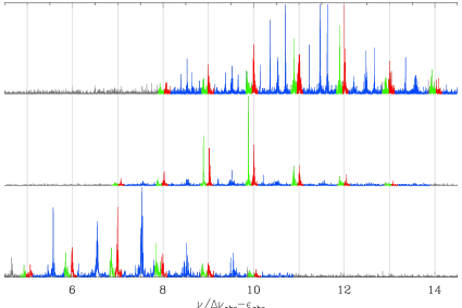
Figure 1: Red giant oscillation spectra, as a function of the normalized frequency; $\ell=0$, 1, and 2 modes are plotted in red, blue, and green, respectively. Top: typical pattern with a large number of gravity-dominated mixed modes. Middle: dipole modes are depressed. Bottom: dipole modes are mostly pressure-dominated.

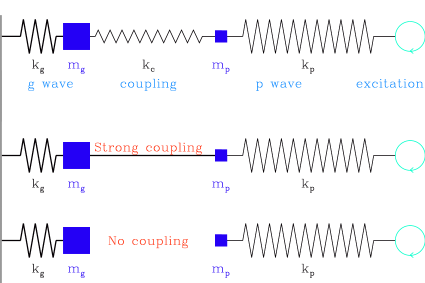
Figure 2: Toy model with two masses and three springs, representative of the coupling of gravity and pressure waves. Top: the mean case, with an intermediate coupling, helps explain the gravity-dominated mixed modes. Middle: very strong coupling; this case provides an explanation of depressed mixed modes. Bottom: very weak coupling; in this case, only pressure modes are observed.

3.3 Gravity dominated, pressure dominated, and depressed dipole mixed modes

The dipole modes observed in red giants show a large variety of oscillation patterns (Fig. 1). Except at low $\nu_{\mathrm{max}}$, all these patterns show a large number of gravity-dominated mixed modes that follow the mixed-mode asymptotic expansion (Eq. 4). The amplitudes of these modes also show a large variety of cases: dipole mixed modes have very low amplitudes for a family of stars identified by [Mosser et al. (2012a)]; in other cases analyzed by [Mosser et al. (2012b)], red giants present a rich dipole pattern with a large number of gravity-dominated mixed modes; in other cases, the pattern is practically limited to the pressure-dominated mixed modes. Apart from the modelling effort to interpret such mixed modes (Dupret et al. 2009, for massive stars), we propose a simple mechanical model for trying to understand the different cases, including the depressed mixed modes.

In this toy-model, we consider a chain of three springs and two masses, as indicated in Fig. 2. The stiffness and the mass that, respectively, represent the p and g modes have to fulfil the resonance condition: $\omega^{2}=k_{\mathrm{p}}/m_{\mathrm{p}}=k_{\mathrm{g}}/m_{\mathrm{g}}$. The masses $m_{\mathrm{p}}$ and $m_{\mathrm{g}}$ are representative of the pressure and gravity mode inertia, respectively. This implies that $m_{\mathrm{g}}\gg m_{\mathrm{p}}$, since the inertia of gravity modes is much higher than the inertia of pressure modes. This means that, accordingly, the stiffness $k_{\mathrm{g}}$ of the gravity spring is much stronger than the stiffness $k_{\mathrm{p}}$ of the pressure spring. The stiffness of the coupling spring is, as one can imagine, representative of the coupling (note that this coupling has an energetic meaning, contrary to the phase coupling factor discussed above). Finally, the excitation mechanism occurs at the extremity of the pressure spring, in order to mimic the free surface of the oscillation and the location of the excitation in the uppermost level. The opposite extremity of the gravity spring is fixed; it corresponds to the barycenter of the star.

This toy model can be used to understand typical observations. We first examine the most common case, where a large number of gravity-dominated mixed modes are observed (Fig. 1). We then investigate two opposite (and extreme) cases corresponding to the case where the amplitudes of gravity-dominated mixed modes are severely damped, or to the case where only pressure-dominated mixed modes are seen:

- The common case corresponds to a ‘moderate’ coupling. In the transitory regime, the coupling is low enough to ensure the efficient excitation of pressure waves: the energy input from the oscillation is not significantly perturbed by the leak through the coupling. In a permanent regime, these (p-)waves have enough energy to excite then gravity waves. Therefore, the model helps understand the gravity dominated mixed modes. The stiffness $k_{\mathrm{c}}$ of the coupling spring is low enough to allow significant amplitudes of the p mode, but high enough to regulate the frequency of this p mode by the much more stable gravity oscillator. Depending on the frequency, the resulting modes are dominated either by pressure or gravity.

- A tight coupling corresponds to a very high coupling stiffness. In that case, we can consider that the masses $m_{\mathrm{p}}$ and $m_{\mathrm{g}}$ are bound together. Since $k_{\mathrm{g}}\gg k_{\mathrm{p}}$, no significant movement is expected: the excitation at the surface is not efficiently transmitted to $m_{\mathrm{p}}$ and $m_{\mathrm{g}}$ since they are in practice tightly attached by $k_{\mathrm{g}}$ with the immobile center. The excitation is inefficient: the waves excited at the surface cannot reach great amplitudes since that they have to move a very high inertia. Even the pressure-dominated modes cannot form. It is straightforward to consider that the depressed mixed modes, with limited oscillation amplitudes, correspond to this strong-coupling case. This might correspond to a reduced region between the pressure and gravity cavity. In other words, the Brunt-Väisälä (BV) and $\ell=1$ Lamb (L1) frequencies have close values, which are also close to the frequency of the damped modes. If the BV frequency exceeds the Lamb frequency, one may suppose that, with pressure and buoyancy acting as restoring forces, the coupling will be extremely efficient.

- An inefficient coupling is ensured by an absence of the coupling spring. In that case, the excitation is able to move $m_{\mathrm{p}}$ without any reaction of $m_{\mathrm{g}}$. This case corresponds to oscillation spectra without important gravity dominated peaks. Such a coupling may correspond to a wide region between the BV and L1 cavities. In that case, gravity waves cannot be excited.

In this model, it is possible to suppose, as in the real case, that the power density of the excitation only weakly depends on frequency. All mixed modes associated to the same pressure mode have then similar height in a power density spectrum. They just differ by their lifetime. A condition to reach uniform height is the observation duration, which has to be high enough, higher than the mixed-mode lifetimes, in order to observe resolved modes.

Finally, this model helps understand the energy partition reported by [Mosser et al. (2012a)]. The excitation taking place in the uppermost envelope is transferred towards the stellar core by p waves only. The total energy that could be affected to one single p mode is shared between all mixed modes associated to this p mode. This partition is efficient in most cases, when the coupling between the waves in the two cavities is moderate. A high coupling induces an important consequence: the dipole modes have a much higher inertia than radial modes, so that their surface amplitudes are totally damped.

3.4 Rotation and mixed modes

Rotational splittings observed in a handful of giants have first exhibited the significant radial differential rotation in the red giants interior (Beck et al. 2012, Deheuvels et al. 2012): the inner rotation rate is significantly higher than the envelope rotation rate. Then, the analysis of $\simeq\,300$ spectra by [Mosser et al. (2012b)] has shown the spin-down of the mean core rotation when red giant ascent the RGB. This spin-down is more pronounced for more-evolved stars in the red clump.

[Marques et al. (2013)] have established seismic diagnostics for transport of angular momentum in stars from the pre-main sequence to the red-giant branch. They found that transport by meridional circulation and shear turbulence yields far too high a core rotation rate for red-giant models compared with observations. Either turbulent viscosity is largely underestimated, or a mechanism not included in current stellar models of low mass stars is needed to slow down the core rotation. [Goupil et al. (2013)] have derived a theoretical framework for understanding the properties of the observed rotational splittings of red giant stars with slowly rotating cores. They were then able to describe the morphology of the rotational splittings, under the hypothesis of linear splittings. In fact, the mean core rotation dominates the splittings, even for pressure dominated mixed modes. As a consequence, they provided theoretical support for using a Lorentzian profile to measure the observed splittings of red giant stars. [Ouazzani et al. (2013)] have shown the complexity of the splittings when rotation cannot be considered as a perturbation. When rotational splitting are higher than twice the frequency separation between consecutive dipolar modes, non-perturbative computations are necessary. Each family of modes with different azimuthal symmetry $m$ has to be considered separately. In case of rapid core rotation, the differences between the period spacings associated with a given azimuthal order $m$ constitutes a promising guideline toward a proper seismic diagnostic for rotation.

Observing rotational splittings at lower frequencies than reported by [Mosser et al. (2012b)] is challenging. First, such an observation requires the presence of gravity-dominated mixed modes. At low $\nu_{\mathrm{max}}$, such modes have so long lifetimes that very long observations are necessary to unveil them. Second, disentangling mixed-mode spacing and rotational splitting at low $\nu_{\mathrm{max}}$ is demanding, especially for RGB stars. We shall consider, as an example, an RGB star that has $\Delta\nu=4\,\mu$Hz and $\nu_{\mathrm{max}}=35\,\mu$Hz; such a star has to be distinguished from its more evolved counterpart in the red clump, which has similar $\Delta\nu$ and $\nu_{\mathrm{max}}$. Such a RGB star has a period spacing $\Delta\Pi_{1}\simeq 50\pm 3$ s. The extrapolation of the measurements in [Mosser et al. (2012b)] provides a rotational splitting $\delta\nu_{\mathrm{rot}}$ in the range [200 – 300 nHz]. At $\nu_{\mathrm{max}}$, the frequency spacing associated to $\Delta\Pi_{1}$ is of the order of 70 nHz. This means that the multiplet components of 6 to 9 radial orders are superimposed in a same small frequency range. Disentangling them will be highly difficult, if not impossible.

4 Conclusion

At the time this paper is written, red giant seismology is still in progress. It is however clear that we have efficient tools for analyzing the spectra. The universal red giant oscillation pattern has proven to provide the most precise measurement of the large separation; furthermore, it provides the full identification of the modes, i.e. their radial order and angular degree. The asymptotic expansion for mixed modes has proven to precisely depict the dipole mixed-mode pattern. The observation of large gravity radial orders ensures a precise measurement of the gravity-mode spacing. The toy model describing the coupling of pressure and gravity waves allows us to better understand the mixed modes.

The efficient work done by the CoRoT and Kepler red giant working groups ensures a permanent flux of new discoveries. Intensive work is in progress, for a thorough understanding of global and individual properties of red giants: ensemble seismology, interior structure, stellar physics, astrophysical consequences for stellar population or Galactic physics.

With dipole mixed modes, we have an efficient way to extract information from the stellar core. With gravity period spacings, we can explore the physics of the stellar core, including the nuclear reactions at the different evolutionary stages. With the rotational splittings, we can explore the inner angular momentum and its evolution in red giants. With the observation of depressed mixed modes, we can identify and study stars with very close Brunt-Väisälä and Lamb cavities.

The accuracy of scaling relations providing the stellar mass and radius is enhanced by all the calibration work. This calibration can be done with theoretical work (Belkacem et al. 2011), with specific studies of cluster stars (Miglio et al. 2012), or by modelling (Belkacem et al. 2013). This modelling work shows that, following [Mosser et al. (2013a)], it is necessary to distinguish between the large separation observed at $\nu_{\mathrm{max}}$, the asymptotic value, and the dynamical frequency which scales as $\sqrt{M/R^{3}}$.

All this study relied on a set of about 1400 red giants studied since [Bedding et al. (2010)]. The amount of data will be increased by a factor of twenty with CoRoT data and Kepler public data (Stello et al. 2013).

- [1]
- [Beck et al. (2011)] Beck, P. G., Bedding, T. R., Mosser, B., et al. 2011, Science, 332, 205
- [Beck et al. (2012)] Beck, P. G., Montalban, J., Kallinger, T., et al. 2012, Nature, 481, 55
- [Bedding et al. (2010)] Bedding, T. R., Huber, D., Stello, D., et al. 2010, ApJ Letters, 713, L176
- [Bedding et al. (2011)] Bedding, T. R., Mosser, B., Huber, D., et al. 2011, Nature, 471, 608
- [Belkacem et al. (2011)] Belkacem, K., Goupil, M. J., Dupret, M. A., et al. 2011, A&A, 530, A142
- [Belkacem(2012)] Belkacem, K. 2012, in SF2A-2012: Proceedings of the Annual meeting of the French Society of Astronomy and Astrophysics, ed. S. Boissier, et al. 173–188
- [Belkacem et al. (2013)] Belkacem, K., Samadi, R.; Mosser, B., et al. 2013, 2013arXiv1307.3132B
- [Benomar et al. (2013)] Benomar, O.; Bedding, T. R.; Mosser, B., et al. 2013, ApJ, 767, 158
- [Corsaro et al. (2012)] Corsaro, E., Stello, D., Huber, D., et al. 2012, ApJ, 757, 190
- [De Ridder et al.(2009)De Ridder, Barban, Baudin, Carrier, Hatzes, Hekker, Kallinger, Weiss, Baglin, Auvergne, Samadi, Barge, & Deleuil] De Ridder, J., Barban, C., Baudin, F., et al. 2009, Nature, 459, 398
- [Deheuvels et al. (2012)] Deheuvels, S., García, R. A., Chaplin, W. J., et al. 2012, ApJ, 756, 19
- [Di Mauro et al. (2011)] di Mauro, M. P.; Cardini, D.; Catanzaro, G et al. 2011, MNRAS 415, 3783
- [Dupret et al. (2009)] Dupret, M., Belkacem, K., Samadi, R., et al. 2009, A&A, 506, 57
- [Goupil et al. (2013)] Goupil, M. J., Mosser, B., Marques, J. P., et al. 2013, A&A, 549, A75
- [Hekker et al. (2011)] Hekker, S., Elsworth, Y., De Ridder, J., et al. 2011, A&A, 525, A131
- [Hekker et al. (2012)] Hekker, S., Elsworth, Y., Mosser, B., et al. 2012, A&A, 544, A90
- [Huber et al.(2011)Huber, Bedding, Stello, Hekker, Mathur, Mosser, Verner, Bonanno, Buzasi, Campante, Elsworth, Hale, Kallinger, Silva Aguirre, Chaplin, De Ridder, García, Appourchaux, Frandsen, Houdek, Molenda-Żakowicz, Monteiro, Christensen-Dalsgaard, Gilliland, Kawaler, Kjeldsen, Broomhall, Corsaro, Salabert, Sanderfer, Seader, & Smith] Huber, D., Bedding, T. R., Stello, D., et al. 2011, ApJ, 743, 143
- [Jiang et al. (2011)] Jiang, C., Jiang, B., Christensen-Dalsgaard, J., et al. 2012, ApJ, 742, 120
- [Kallinger et al.(2010)Kallinger, Mosser, Hekker, Huber, Stello, Mathur, Basu, Bedding, Chaplin, De Ridder, Elsworth, Frandsen, García, Gruberbauer, Matthews, Borucki, Bruntt, Christensen-Dalsgaard, Gilliland, Kjeldsen, & Koch] Kallinger, T., Mosser, B., Hekker, S., et al. 2010, A&A, 522, A1
- [Kallinger et al. (2012)] Kallinger, T., Hekker, S., Mosser, B., et al. 2012, A&A, 541, A51
- [Marques et al. (2013)] Marques, J. P., Goupil, M. J., Lebreton, Y., et al. 2013, A&A, 549, A74
- [Mathur et al.(2011)Mathur, Hekker, Trampedach, Ballot, Kallinger, Buzasi, García, Huber, Jiménez, Mosser, Bedding, Elsworth, Régulo, Stello, Chaplin, De Ridder, Hale, Kinemuchi, Kjeldsen, Mullally, & Thompson] Mathur, S., Hekker, S., Trampedach, R., et al. 2011, ApJ, 741, 119
- [Miglio et al. (2010)] Miglio, A., Montalbán, J., Carrier, F., et al. 2010, A&A, 520, L6
- [Miglio et al. (2012)] Miglio, A., Brogaard, K., Stello, D., et al. 2012, MNRAS, 419, 2077
- [Montalbán et al. (2013)] Mosser, B., Michel, E., Belkacem, K., et al. 2013, ApJ, 766, 118
- [Mosser et al. (2008)] Montalbán, J., Miglio, A., Noels, A., et al. 2013, A&A, 478, 197
- [Mosser & Appourchaux(2009)] Mosser, B. & Appourchaux, T. 2009, A&A, 508, 877
- [Mosser (2010)] Mosser, B., 2010, AN, 331, 944
- [Mosser et al.(2010)Mosser, Belkacem, Goupil, Miglio, Morel, Barban, Baudin, Hekker, Samadi, De Ridder, Weiss, Auvergne, & Baglin] Mosser, B., Belkacem, K., Goupil, M., et al. 2010, A&A, 517, A22
- [Mosser et al. (2011a)] Mosser, B., Belkacem, K., Goupil, M., et al. 2011b, A&A, 525, L9
- [Mosser et al.(2011b)Mosser, Barban, Montalbán, Beck, Miglio, Belkacem, Goupil, Hekker, De Ridder, Dupret, Elsworth, Noels, Baudin, Michel, Samadi, Auvergne, Baglin, & Catala] Mosser, B., Barban, C., Montalbán, J., et al. 2011a, A&A, 532, A86
- [Mosser et al. (2012a)] Mosser, B., Elsworth, Y., Hekker, S., et al. 2012a, A&A, 537, A30
- [Mosser et al. (2012b)] Mosser, B., Goupil, M. J., Belkacem, K., et al. 2012c, A&A, 540, A143
- [Mosser et al.(2012c)Mosser, Goupil, Belkacem, Marques, Beck, Bloemen, De Ridder, Barban, Deheuvels, Elsworth, Hekker, Kallinger, Ouazzani, Pinsonneault, Samadi, Stello, García, Klaus, Li, Mathur, & Morris] Mosser, B., Goupil, M. J., Belkacem, K., et al. 2012b, A&A, 548, A10
- [Mosser (2013)] Mosser, B., 2013, European Physical Journal Web of Conferences, 43
- [Mosser et al. (2013a)] Mosser, B., Michel, E., Belkacem, K., et al. 2013, A&A, 550, A126
- [Mosser et al. (2013b)] Mosser, B., Samadi, R., Belkacem, K., 2013, in SF2A-2013
- [Ouazzani et al. (2013)] Ouazzani, R.-M. and Goupil, M. J. and Dupret, M.-A. and Marques, J. P., A&A, 554, A80
- [Roxburgh & Vorontsov(2006)] Roxburgh, I. W., & Vorontsov, S. V. 2006, MNRAS, 369, 1491
- [Samadi et al.(2012)Samadi, Belkacem, Dupret, Ludwig, Baudin, Caffau, Goupil, & Barban] Samadi, R., Belkacem, K., Dupret, M.-A., et al. 2012, A&A, 543, A120
- [Samadi et al.(2010)Samadi, Ludwig, Belkacem, Goupil, & Dupret] Samadi, R., Ludwig, H.-G., Belkacem, K., Goupil, M. J., & Dupret, M.-A. 2010, A&A, 509, A15
- [Tassoul (1980)] Tassoul, M. 1980, ApJS, 43, 469
- [Unno et al. (1989)] Unno, W., Osaki, Y., Ando, H., Saio, H., & Shibahashi, H. 1989, Nonradial oscillations of stars, ed. Unno, W., Osaki, Y., Ando, H., Saio, H., & Shibahashi, H. (University of Tokyo Press)
- [Verner et al. (2011)] Verner, G. A., Elsworth, Y., Chaplin, W. J., et al. 2011, MNRAS, 415, 3539
- [White et al.(2011)White, Bedding, Stello, Christensen-Dalsgaard, Huber, & Kjeldsen] White, T. R., Bedding, T. R., Stello, D., et al. 2011, ApJ, 743, 161