Towards Energy Neutrality in Energy Harvesting Wireless Sensor Networks: A Case for Distributed Compressive Sensing?

Abstract

This paper advocates the use of the emerging distributed compressive sensing (DCS) paradigm in order to deploy energy harvesting (EH) wireless sensor networks (WSN) with practical network lifetime and data gathering rates that are substantially higher than the state-of-the-art. In particular, we argue that there are two fundamental mechanisms in an EH WSN: i) the energy diversity associated with the EH process that entails that the harvested energy can vary from sensor node to sensor node, and ii) the sensing diversity associated with the DCS process that entails that the energy consumption can also vary across the sensor nodes without compromising data recovery. We also argue that such mechanisms offer the means to match closely the energy demand to the energy supply in order to unlock the possibility for energy-neutral WSNs that leverage EH capability. A number of analytic and simulation results are presented in order to illustrate the potential of the approach.

I Introduction

Future deployments of wireless sensor network (WSN) infrastructures are expected to be equipped with energy harvesters (e.g. piezoelectric, thermal or photovoltaic) to substantially increase their autonomy and lifetime [1, 2, 3]. However, it is also widely recognized that the existing gap between the sensors’ energy harvesting (EH) supply and the sensors’ energy demand is not likely to close in the near future due to limitations in current EH technology, together with the surge in demand for more data-intensive applications [3]. Consequently, the realization of energy neutral (or nearly energy neutral) WSNs for data-intensive applications remains a very challenging problem.

These considerations have motivated the design of various emerging data acquisition and transmission schemes and protocols for EH WSNs [1, 4, 5]. For example, [1] proposes to characterize the complex time varying nature of energy sources with analytically tractable models, [4] proposes energy management policies that are throughput optimal and mean delay optimal, and [5] puts forth a directional water-filling algorithm that maximizes the throughput by a deadline, and minimizes the transmission completion time of the communication session. However, such existing energy management approaches do not integrate organically fundamental mechanisms associated with the EH process and the sensing process in an EH WSN: energy diversity and sensing diversity.

This article – at the core of its contribution – advocates the use of distributed compressive sensing (DCS) in order to deploy WSNs with practical network lifetime and data gathering rates that are substantially higher than the state-of-the-art. The key attributes of the proposed approach that lead to efficient energy management are associated with the fact that – subject to certain conditions on the measurement process and the collection of signals to be sensed (e.g., intra- and inter-signal correlation) –
– the number of data projections (measurements) at the various sensors can be substantially lower than the data dimensionality without compromising data recovery [6, 7];
– the number of data projections (measurements) at the various sensors can be adjusted without compromising data recovery [8, 9].
Since the number of projections acts as a proxy to energy efficiency – in view of the fact that transmission energy tends to be orders of magnitude higher than sensing/computational energy in various WSNs applications [10, 11] – then the proposed approach provides for i) substantial energy efficiency in relation to other approaches, such as methods that do not exploit any form of source compression; and ii) adapting energy consumption to the random nature of energy availability in EH systems.

That is, the article argues that – due to the energy diversity associated with the EH process where the harvested energy can vary from sensor to sensor and the sensing diversity associated with the DCS process where the number of projections can also vary from sensor to sensor – one should able to closely match the energy supply to the energy demand in order to unlock the possibility for energy neutral operation in EH WSNs. This principle is illustrated in the sequel: Section II describes in detail the proposed sensing approach. Sections III and IV present analytic and simulation results that support the potential of the approach. General concluding remarks are drawn in Section V.

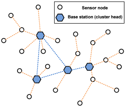
Figure 1: A typical cluster-based WSN architecture.

Figure 2: Typical energy consumption profile of a data acquisition and EH scheme.

II System Description

We consider a typical cluster-based WSN architecture, as shown in Fig. 1, where a set of sensor nodes (SNs) periodically conveys data to one or more base stations (BSs). We assume slotted transmission such that within a time slot of $T$ seconds the SNs are active for $T_{\text{act}}$ seconds in order to capture and transmit data and are inactive for $T-T_{\text{act}}$ seconds in order to harvest energy from the environment, as shown in Fig. 2. We also consider an innovative data gathering and reconstruction process – which is key to match the energy demand to the energy supply – based on three key steps: i) DCS based data acquisition, ii) transmission of projections, and iii) DCS based data reconstruction.

II-A Data Acquisition

The SNs capture low-dimensional projections of the original high-dimensional data during each activation time $iT-T_{\text{act}}\leq t\leq iT$, which are given by:

$$\mathbf{y}_{k}(i)=\mathbf{\Phi}_{k}(i)\mathbf{f}_{k}(i),$$ (1)

where $\mathbf{y}_{k}(i)\in\mathbb{R}^{m_{k}(i)}$ is the projections vector at the $k$th SN corresponding to the $i$th time interval, $\mathbf{f}_{k}(i)\in\mathbb{R}^{n(i)}$ is the original (Nyquist-sampled) data vector at the $k$th SN corresponding to the $i$th time interval, and $\mathbf{\Phi}_{k}(i)\in\mathbb{R}^{m_{k}(i)\times n(i)}$ is the projections matrix where $m_{k}(i)\ll n(i)$ for any time interval $i$ and SN $k$. Note that the dimensionality of the projections can vary in different activation times and different sensor nodes. In practice, one may obtain the projections vector from the original data signal using analogue CS encoders [10, 12], whereby the projections vector is obtained directly from the analogue continuous-time data, or using digital CS encoders [10], whereby the projections vector is obtained from the Nyquist sampled discrete-time data via (1). Recent studies suggest that digital CS encoders are more energy efficient than analogue CS encoders for WSNs [10].

II-B Data Transmission

The SNs then convey the low-dimensional projections of the original high-dimensional data to the respective fusion centers. We assume that upon activation the SNs converge into a balanced time-frequency steady-state mode where each SN is associated with a BS using a particular channel (or joins a synchronized channel hopping schedule) in order to convey data without collisions. We also assume that fading, external interference noise and other non-idealities in packet transmissions are dealt with via the PHY layer modulation and coding mechanisms of standards like IEEE 802.15.4. Therefore, the transmission of the projections of the original data is taken to be essentially perfect without a significant loss in generality.

II-C DCS Based Data Reconstruction

We take the signals $\mathbf{f}_{k}(i)\in\mathbb{R}^{n(i)}$ to admit a sparse representation $\mathbf{x}_{k}(i)\in\mathbb{R}^{n(i)}$ in some basis $\mathbf{\Psi}(i)\in\mathbb{R}^{n(i)\times n(i)}$, i.e.

$$\mathbf{f}_{k}(i)=\mathbf{\Psi}(i)\mathbf{x}_{k}(i),$$ (2)

where $\|\mathbf{x}_{k}(i)\|_{0}=s_{k}(i)\ll m_{k}(i)\ll n(i)$. In addition, we also take the sparse representations to obey the sparse common component and innovations (SCCI) model that has been frequently used to capture intra- and inter-signal correlation typical of physical signals (e.g., temperature, humidity) in WSNs [8], i.e.,

$$\mathbf{x}_{k}(i)=\mathbf{z}_{c}(i)+\mathbf{z}_{k}(i),$$ (3)

where $\mathbf{z}_{c}(i)\in\mathbb{R}^{n(i)}$ with $\|\mathbf{z}_{c}(i)\|_{0}=s_{c}^{\prime}(i)\ll n(i)$ denotes the common component of the sparse representation $x_{k}(i)\in\mathbb{R}^{n(i)}$, which is common to the various SNs, and $z_{k}(i)\in\mathbb{R}^{n(i)}$ with $\|\mathbf{z}_{k}(i)\|_{0}=s_{k}^{\prime}(i)\ll n(i)$ denotes the innovations component of the sparse representation $x_{k}(i)\in\mathbb{R}^{n(i)}$, which is specific to each SN. Note that $s_{c}^{\prime}(i)+s_{k}^{\prime}(i)\geq s_{k}(i)$.

The typical signal reconstruction process behind conventional CS approaches involves solving the following optimization problem to recover individually the original signals captured by the various sensors:

$$\begin{split}\min_{\mathbf{x}_{k}(i)}\qquad&\|\mathbf{x}_{k}(i)\|_{1}\\ \text{s.t.}\qquad&\mathbf{A}_{k}(i)\mathbf{x}_{k}(i)=\mathbf{y}_{k}(i),\end{split}$$ (4)

where $\mathbf{A}_{k}(i)=\mathbf{\Phi}_{k}(i)\mathbf{\Psi}(i)\in\mathbb{R}^{m_{k}(i)\times n(i)}$.

In contrast, the signal reconstruction process behind the adopted DCS approach involves solving the following optimization problem to recover jointly the original signals captured by various SNs:

$$\begin{split}\min_{\tilde{\mathbf{z}}(i)}\qquad&\|\tilde{\mathbf{z}}(i)\|_{1}\\ \text{s.t.}\qquad&\tilde{\mathbf{A}}(i)\tilde{\mathbf{z}}(i)=\tilde{\mathbf{y}}(i),\end{split}$$ (5)

where $\tilde{\mathbf{z}}(i)=\left[\mathbf{z}_{c}(i)^{T}\ \mathbf{z}_{1}(i)^{T}\ \ldots\ \mathbf{z}_{K}(i)^{T}\right]^{T}\in\mathbb{R}^{(K+1)n(i)}$ is the extended sparse signal vector, $\tilde{\mathbf{y}}(i)=\left[\mathbf{y}_{1}(i)^{T}\ \ldots\ \mathbf{y}_{K}(i)^{T}\right]^{T}\in\mathbb{R}^{\sum_{k=1}^{K}m_{k}(i)}$ is the extended measurements vector, and $\tilde{\mathbf{A}}(i)\in\mathbb{R}^{\left(\sum_{k=1}^{K}m_{k}(i)\right)\times(K+1)n(i)}$ is the extended sensing matrix given by

$$\tilde{\mathbf{A}}(i)=\begin{bmatrix}\mathbf{A}_{1}(i)&\mathbf{A}_{1}(i)&\mathbf{0}&\mathbf{0}&\cdots&\mathbf{0}\\ \mathbf{A}_{2}(i)&\mathbf{0}&\mathbf{A}_{2}(i)&\mathbf{0}&\cdots&\mathbf{0}\\ \vdots&&&&\ddots&\vdots\\ \mathbf{A}_{K}(i)&\mathbf{0}&\mathbf{0}&\mathbf{0}&\cdots&\mathbf{A}_{K}(i)\end{bmatrix}.$$

Note that the reconstruction procedure in (5) – in contrast to the reconstruction procedure in (4) – exploits not only intra- but also inter-signal correlation in order to provide further efficiency gains that are leveraged by our DCS based energy management scheme.

II-D Energy Consumption and Harvesting Models

The data gathering process is subject to a causal energy harvesting constraint. In particular, we assume that the SNs have to obey a certain energy budget during each activation interval $iT-T_{\text{act}}\leq t\leq iT$, which is given by:

$$\xi_{k}(i)=\min\left\{\xi_{k}^{\texttt{tot}};\left(\sum_{j\leq i}\xi_{k}^{H}(j)\right)-\left(\sum_{j<i}\xi_{k}^{C}(j)\right)\right\},$$ (6)

where $\xi_{k}^{\texttt{tot}}$ is the capacity of the battery of SN $k$, $\xi_{k}^{H}(j)$ is the energy harvested by SN $k$ in the interval $(j-1)T\leq t\leq jT-T_{\text{act}}$ and $\xi_{k}^{C}(j)$ is the energy consumed by SN $k$ in the interval $jT-T_{\text{act}}\leq t\leq jT$. Note that this budget is positive because the cumulative consumed energy has to be less than the cumulative harvested energy.

We adopt the following models that are relevant to determine the energy harvested and the energy consumed in each activation interval. We assume that energy consumed for sensing, computing and transmitting one measurement is a constant $\tau>0$. Hence, the energy budget $\xi_{k}(i)$ for transmitting $m_{k}(i)$ measurements should satisfy:

$$\xi_{k}(i)\geq\tau m_{k}(i).$$ (7)

We also assumed that the harvested power follows a uniform distribution in the interval $[(1-\rho)\mu,(1+\rho)\mu]$, where $\mu$ denotes the mean harvested power and $0<\rho\leq 1$. We adopt this particular simple model in view of the fact that power harvesting with current technologies for solar and piezoelectric harvesters is either piecewise uniformly distributed (or a mixture of two uniform probability density functions (PDFs) around the peak harvesting and minimal harvesting values) or simply uniformly distributed over the range of power that can be generated by the energy harvester [1, 2, 3]. For example, piezoelectric harvesting with a 1 $\texttt{cm}^{2}$ panel can be assumed to derive power that is piecewise uniformly distributed between $[0,200\mu\texttt{W}]$, or simply uniformly distributed within this range [3].

We also adopt throughout a very simple energy management approach where the SNs use the entire available energy budget per activation interval, i.e., the number of projections per SN are such that the energy consumption fits into the harvested energy budget (the unused energy is taken to be lost from one activation interval to a subsequent one). Therefore, we drop the activation interval index $i$ in the ensuing analysis to simplify the notation.

III Towards Energy Neutrality: an Analysis of the Two Sensor Scenario

We illustrate the essence of the approach in an EH WSN consisting of two SNs, where the energy harvested by each SN is independent. We compare the main attributes of the DCS data gathering scheme to a CS and a raw data acquisition method.

The simplicity of the two sensor scenario unveils the potential of the DCS approach to unlock higher levels of energy efficiency in EH WSNs.

III-A Raw Data Gathering Scheme

The probability of incorrect data reconstruction in a raw data gathering scheme can be lower bounded by the probability that the energy harvested by the two SNs is not sufficient to fit the energy consumption requirements by each of the two SNs. Hence, by using the assumption that the EH processes follow independent uniform distributions in the interval $[(1-\rho)\mu,(1+\rho)\mu]$ it follows that the probability of incorrect data collection due to energy depletion can be lower bounded as follows:

$$\begin{split}\emph{P}_{\texttt{raw}}&\geq 1-\emph{P}\left(\xi_{1}\geq n\tau,\xi_{2}\geq n\tau\right)\\ &=1-\left(\frac{(1+\rho)\mu-n\tau}{2\rho\mu}\right)^{2}.\end{split}$$ (8)

III-B CS Data Acquisition Scheme

We now consider the probability of incorrect data reconstruction in a CS based data acquisition scheme by assuming that the signals sensed by the two sensors exhibit the same sparsity level, i.e. $s=s_{1}=s_{2}$. In particular, we use the fact that $m_{k}\approx c\left(s_{k},n\right)=\mathcal{O}\left(s_{k}\log\frac{n}{s_{k}}\right)$ where $m_{k}\leq n$ is a necessary (and sufficient) condition for the successful reconstruction of the sparse signals via the $\ell_{1}$-norm minimization problem in (4) [13]. Therefore, by using the assumption that the EH processes follow independent uniform distributions in the interval $[(1-\rho)\mu,(1+\rho)\mu]$, we can also lower bound the probability of incorrect data reconstruction as follows:

$$\begin{split}\emph{P}_{\texttt{CS}}&\geq 1-\emph{P}\left(\xi_{1}\geq m_{1}\tau,\xi_{2}\geq m_{2}\tau\right)\\ &=1-\left(\frac{(1+\rho)\mu-c(s,n)\tau}{2\rho\mu}\right)^{2}.\end{split}$$ (9)

III-C DCS Data Acquisition Scheme

We finally consider the probability of incorrect data reconstruction in a DCS based data acquisition scheme by assuming that the signals sensed by the two sensors exhibit a certain common support size $s_{c}^{\prime}$ and the same innovation support size, i.e., $s^{\prime}=s_{1}^{\prime}=s_{2}^{\prime}$. We now use the fact that

$$m_{k}\approx c\left(\hat{s},n\right)\qquad k=1,2,$$ (10)

where $\hat{s}=2s^{\prime}-\frac{s^{\prime 2}}{n}$ and

$$m_{1}+m_{2}\approx c\left(\hat{s},n\right)+c\left(\tilde{s},n\right)$$ (11)

where $\tilde{s}=s_{c}^{\prime}+2s^{\prime}-\frac{2s_{c}^{\prime}s^{\prime}}{n}-\frac{s^{\prime 2}}{n}+\frac{s_{c}^{\prime}s^{\prime 2}}{n^{2}}$, are necessary conditions for the joint successful reconstruction of the two sparse signals via the joint $\ell_{1}$ reconstruction algorithm in (5) [8]. Therefore, we can also lower bound the probability of incorrect data reconstruction by using the assumption that the EH processes follow independent uniform distributions in the interval $[(1-\rho)\mu,(1+\rho)\mu]$ as follows:

$$\begin{split}&\emph{P}_{\texttt{DCS}}\geq 1-\emph{P}\left(\xi_{1}\geq c\left(\hat{s},n\right)\tau,\ \xi_{2}\geq c\left(\hat{s},n\right)\tau,\right.\\ &\qquad\qquad\qquad\left.\xi_{1}+\xi_{2}\geq c\left(\hat{s},n\right)\tau+c\left(\tilde{s},n\right)\tau\right)\\ &\geq 1-\emph{P}\left(\xi_{1}+\xi_{2}\geq c\left(\hat{s},n\right)\tau+c\left(\tilde{s},n\right)\tau\right)\\ &=\left\{\begin{array}[]{cl}\frac{1}{2}\left(\frac{m^{\prime}\tau-2(1-\rho)\mu}{2\rho\mu}\right)^{2}&\quad\texttt{if}\ m^{\prime}\tau\leq 2\mu\\ 1-\frac{1}{2}\left(\frac{2(1+\rho)\mu-m^{\prime}\tau}{2\rho\mu}\right)^{2}&\quad\texttt{if}\ m^{\prime}\tau>2\mu\end{array},\right.\end{split}$$ (12)

where $m^{\prime}=c\left(\hat{s},n\right)+c\left(\tilde{s},n\right)$.

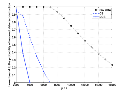
Figure 3: Lower Bound to the probability of incorrect reconstruction vs. $\mu/\tau$ ($\rho=0.5$, $n=10^{4}$, $s=10^{3}$, $s^{\prime}=200$ and $s_{c}^{\prime}=800$).

The fact that the lower bounds to the probability of incorrect data reconstruction for the raw data gathering scheme in (8) or the CS data gathering scheme in (9) are higher than the lower bound to the probability of incorrect data reconstruction for the DCS data acquisition scheme in (12) suggests that our proposed approach leads to better reconstruction quality. These probability bounds are compared in Fig. 3 by using the approximation to the overmeasuring factor $c\left(s_{k},n\right)=s_{k}\log_{2}\left(1+\frac{n}{s_{k}}\right)$ in [8].

III-D Towards Energy Neutrality: Matching Energy Demand to the Energy Supply

The essence of the mechanism that offer the means to match the energy demand to the energy supply at each SN in order to unlock energy neutrality is embodied in (10) and (11): it is clear that – together with the fact that the value of right hand side of (10) is lower than the value of the right hand side of (11) – one can strike a trade-off between the number of measurements taken by the two SNs in order to adapt the energy consumption to the energy availability at any particular node without compromising the data reconstruction quality. That is, such a “sensing diversity” mechanism which is linked to the DCS data gathering process is key to adapt to the “energy diversity” mechanism which is linked to the EH process in order to guarantee successful data recovery.

It is also relevant to reflect on how some of the results may generalize with the increase in the number of SNs in the network. It is clear that the probability that energy supply is not sufficient for the energy demand increases substantially with the increase in the number of SNs in the WSN. Hence, the probability of incorrect data reconstruction associated with the CS based data acquisition scheme (and the raw one) also increases with the increase in the number of nodes. In contrast, the probability of incorrect data reconstruction associated with the DCS based data acquisition scheme exhibits a completely different behavior: such a probability decreases with the increase in the number of nodes until a certain optimum value of SNs; and it then increases with the increase in the number of nodes past the optimum value of SNs.

The roots for such a behavior are linked to the interplay between the level of energy diversity and the level of sensing diversity. For a number of SNs less than the optimal value of SNs the common component in the SCCI model guarantees that there is enough ”sensing diversity” in order to match the energy demand to the variability of the energy supply. For a number of SNs higher than the optimal value of SNs the innovations component in the SCCI model gradually compromises the level of ”sensing diversity”. The exact optimal value of SNs then depends on the exact levels of sparsity in the common and innovations components of the adopted model.

Such a behavior is crisply illustrated in the sequel by considering experiments both with synthetic and real data.

IV Experimental Study

We now illustrate the potential of the approach both with synthetic data and real data collected by the WSN located in the Intel Berkeley Research Lab [14].

IV-A Synthetic Experiments

In the synthetic experiments, we generate the sparse signal representations $\mathbf{x}_{k}$ ($k=1,\ldots,K$) randomly with ambient dimension $n=50$ are generated randomly, where the non-zero components are drawn from independent identically distributed (i.i.d.) Gaussian distribution $\mathcal{N}(0,1)$. We also generate the equivalent sensing matrices $\mathbf{A}_{k}$ ($k=1,\ldots,K$) randomly, where the elements are also drawn from i.i.d. Gaussian distribution $\mathcal{N}(0,1)$.

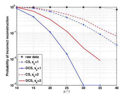
Figure 4: Probability of incorrect reconstruction vs. $\mu/\tau$ ($K=2$ and $s_{c}^{\prime}=5$).

Fig. 4 shows the probability of incorrect data reconstruction vs. the energy availability level for the different data gathering mechanisms. We can conclude that for a certain target probability of incorrect data reconstruction the DCS scheme requires less EH capability in relation to the CS or the raw data scheme or – conversely – for a certain EH capability the proposed scheme leads to a lower probability of incorrect data reconstruction in relation to the other schemes. For example, for probability of incorrect reconstruction equal to $0.01$, DCS with $s_{k}=1$ requires only $26\tau$ while CS require $34\tau$, and raw data transmission requires orders of magnitude higher than DCS in terms of mean energy availability. We can also conclude that – as argued in the previous section - that the sparsity level of the innovations component of the SCCI model has a considerable effect on the trends and results.

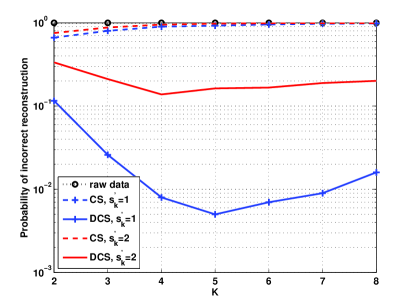
Figure 5: Probability of incorrect reconstruction vs. number of SNs $K$ ($\mu=20\tau$, $s_{c}^{\prime}=4$ and $s_{k}^{\prime}=1$).

Fig. 5 shows the probability of incorrect data reconstruction vs. the number of SNs in the EH WSN. This Figure confirms that the probability of incorrect reconstruction with CS increases as the number of SNs grows, since a larger number of SNs yields a higher risk that some SN will fail to harvest enough energy for acquiring the necessary number of measurements for successful reconstruction. Conversely, the probability of incorrect reconstruction with the DCS approach first decreases and then increase as the the number of SNs grows. This trend – as argued earlier – depends on the interplay between the level of energy diversity and the level of sensing diversity.

IV-B Experiments With Real Data

In the real data experiments, we illustrate the potential of the paradigm in a simple scenario: temperature monitoring by a WSN located in the Intel Berkeley Research lab [14]. In particular, we only use the contiguous data that was available from $8$ SNs, i.e., SN 2, 3, 4, 7, 8, 9, 10 and 11. We assume the use of a typical 250 kbps 62.64 mW ($17.4\texttt{mA}\times 3.6\texttt{V}$) ZigBee RF transceiver and a solar panel with an average harvesting power 10$\mu\texttt{W/cm}^{2}$ [2]. We also assume that harvested power is uniformly distributed within $[5\mu\texttt{W/cm}^{2},15\mu\texttt{W/cm}^{2}]$. The SN independently and randomly collects a small portion of the original samples and transmits them to the FC based on their availability of harvested energy. All the temperature signals we employ in the following study have a length of $n=512$.

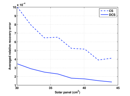
Figure 6: Averaged relative recovery error vs. solar panel size ($K=2$).

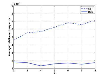
Figure 7: Averaged relative recovery error vs. number of SNs $K$ (solar panel of 40$cm^{2}$ ).

Note that the temperature signals monitored by the WSN are compressible rather than exactly sparse via the discrete cosine transform (DCT). Thus, we use the relative recovery error for a single SN which is equal to $\frac{\|\hat{\mathbf{f}}_{k}-\mathbf{f}_{k}\|_{2}^{2}}{\|\mathbf{f}_{k}\|_{2}^{2}}$, where $\mathbf{f}_{k}$ and $\hat{\mathbf{f}}_{k}$ are the original signal and the reconstructed signal of the $k$th SN respectively rather than the probability of incorrect data reconstruction to evaluate the performance.

Fig. 6 shows the averaged relative recovery error of $K=2$ SNs, i.e., SN 2 and SN 3, achieved by the DCS and the CS data gathering schemes for various solar panel sizes. It is clear that the DCS scheme requires much lower energy levels in relation to the CS scheme for a certain target relative recovery error. For example, for an averaged relative recovery error equal to $3\times 10^{-4}$, DCS requires only $32\ \texttt{cm}^{2}$ solar panel while CS requires a solar panel exceeding $44\texttt{cm}^{2}$ .

Fig. 7 shows the averaged relative recovery error with a solar panel with fixed size achieved by the DCS and the CS schemes for various number of SNs. We note – once again – that the CS scheme fails as the number of SNs increases, but the DCS scheme does not.

To conclude, the settings behind Figs. 6 and 7 are such that the WSN is powered only via the energy harvested from the environment: the fact that DCS based data gathering enables one to collect data without penalties on the data reconstruction error forms the basis of the energy neutrality claims.

V Conclusion and Discussion

It has been established that energy diversity and sensing diversity are two fundamental mechanisms that offer the means to match the energy demand to the energy supply in EH WSNs based on the DCS data acquisition paradigm. It has also been established that DCS based data acquisition paradigm provides substantial gains in energy efficiency for a certain target data reconstruction quality in relation to other approach, e.g. CS based data acquisition.

The potential of the approach has been unveiled for a simple energy management approach, where the SNs choose to use the entire energy budget per activation interval rather than use only a fraction of the energy budget and store the remaining fraction in some local battery. It is clear that such a more refined energy management approach will also yield to further gains.

Finally, it is interesting to point out that the underlying diversity principles are not too dissimilar from the diversity principles in wireless communications: the variability of the wireless channel calls for transmission methods capable of providing robustness; in turn, the variability of the energy harvesting calls instead for robust sensing methods.

References

- [1] A. Kansal, J. Hsu, S. Zahedi, and M. B. Srivastava, “Power management in energy harvesting sensor networks,” ACM Transactions on Embedded Computing Systems, vol. 6, no. 4, p. 32, 2007.
- [2] S. Roundy, D. Steingart, L. Frechette, P. Wright, and J. Rabaey, “Power sources for wireless sensor networks,” Wireless Sensor Networks, pp. 1–17, 2004.
- [3] S. Sudevalayam and P. Kulkarni, “Energy harvesting sensor nodes: Survey and implications,” Communications Surveys & Tutorials, IEEE, vol. 13, no. 3, pp. 443–461, 2011.
- [4] V. Sharma, U. Mukherji, V. Joseph, and S. Gupta, “Optimal energy management policies for energy harvesting sensor nodes,” Wireless Communications, IEEE Transactions on, vol. 9, no. 4, pp. 1326–1336, 2010.
- [5] O. Ozel, K. Tutuncuoglu, J. Yang, S. Ulukus, and A. Yener, “Transmission with energy harvesting nodes in fading wireless channels: Optimal policies,” Selected Areas in Communications, IEEE Journal on, vol. 29, no. 8, pp. 1732–1743, 2011.
- [6] E. Candès, J. Romberg, and T. Tao, “Robust uncertainty principles: Exact signal reconstruction from highly incomplete frequency information,” IEEE Transactions on information theory, vol. 52, no. 2, pp. 489–509, 2006.
- [7] D. Donoho, “Compressed sensing,” IEEE Transactions on Information Theory, vol. 52, no. 4, pp. 1289–1306, 2006.
- [8] D. Baron, M. Wakin, M. Duarte, S. Sarvotham, and R. Baraniuk, “Distributed compressed sensing,” Technical Report ECE-0612, Electrical and Computer Engineering Department, Rice University, Dec. 2006.
- [9] M. F. Duarte, M. B. Wakin, D. Baron, S. Sarvotham, and R. G. Baraniuk, “Bounds on the reconstruction of sparse signal ensembles from distributed measurements,” arXiv preprint arXiv:1102.2677, 2011.
- [10] F. Chen, A. Chandrakasan, and V. Stojanovic, “Design and analysis of a hardware-efficient compressed sensing architecture for data compression in wireless sensors,” Solid-State Circuits, IEEE Journal of, vol. 47, no. 3, pp. 744–756, Mar.
- [11] H. Mamaghanian, N. Khaled, D. Atienza, and P. Vandergheynst, “Compressed sensing for real-time energy-efficient ecg compression on wireless body sensor nodes,” Biomedical Engineering, IEEE Transactions on, vol. 58, no. 9, pp. 2456–2466, 2011.
- [12] M. Mishali, Y. C. Eldar, O. Dounaevsky, and E. Shoshan, “Xampling: Analog to digital at sub-nyquist rates,” Circuits, Devices & Systems, IET, vol. 5, no. 1, pp. 8–20, 2011.
- [13] D. L. Donoho, “High-dimensional centrally symmetric polytopes with neighborliness proportional to dimension,” Discrete and Computational Geometry, vol. 35, pp. 617–652, Mar. 2006.
- [14] P. Bodik, W. Hong, C. Guestrin, S. Madden, M. Paskin, and R. Thibaux. (2004, Feb.) Intel lab data. [Online]. Available: http://db.csail.mit.edu/labdata/labdata.html