Strong Lens Time Delay Challenge: I. Experimental Design

Abstract

The time delays between point-like images in gravitational lens systems can be used to measure cosmological parameters. The number of lenses with measured time delays is growing rapidly; the upcoming Large Synoptic Survey Telescope (LSST) will monitor $\sim 10^{3}$ strongly lensed quasars. In an effort to assess the present capabilities of the community to accurately measure the time delays, and to provide input to dedicated monitoring campaigns and future LSST cosmology feasibility studies, we have invited the community to take part in a “Time Delay Challenge” (TDC). The challenge is organized as a set of “ladders,” each containing a group of simulated datasets to be analyzed blindly by participating teams. Each rung on a ladder consists of a set of realistic mock observed lensed quasar light curves, with the rungs’ datasets increasing in complexity and realism. The initial challenge described here has two ladders, TDC0 and TDC1. TDC0 has a small number of datasets, and is designed to be used as a practice set by the participating teams. The (non-mandatory) deadline for completion of TDC0 was the TDC1 launch date, December 1, 2013. The TDC1 deadline was July 1 2014. Here we give an overview of the challenge, we introduce a set of metrics that will be used to quantify the goodness-of-fit, efficiency, precision, and accuracy of the algorithms, and we present the results of TDC0. Thirteen teams participated in TDC0 using 47 different methods. Seven of those teams qualified for TDC1, which is described in the companion paper II.

.

1. Introduction

As light travels to us from a distant source, its path is deflected by the gravitational fields of intervening matter. The most dramatic manifestation of this effect occurs in strong lensing, when light rays from a single source can take several paths to reach the observer, causing the appearance of multiple images of the same source. These images will typically be magnified in size and thus total brightness (because surface brightness is conserved in gravitational lensing). When the source is variable, the images are observed to vary with delays between them due to the differing path lengths taken by the light and the gravitational potential that it passes through. A common example of such a source in lensing is a quasar, an extremely luminous active galactic nucleus at cosmological distance. From the observations of the image positions, magnifications, and the time delays between the multiple images we can measure the mass structure of the lens galaxy itself (on scales $\geq M_{\odot}$) as well as a characteristic distance between the source, lens, and observer. This “time delay distance” encodes the cosmic expansion rate, which in turn depends on the energy density of the various components in the universe, phrased collectively as the cosmological parameters.

The time delays themselves have been proposed as tools to study massive substructures within lens galaxies (Keeton & Moustakas, 2009), and for measuring cosmological parameters, primarily the Hubble constant, $H_{0}$ (see, e.g., Suyu et al., 2013, for a recent example), a method first proposed by Refsdal (1964). In the future, we aspire to measure further cosmological parameters (e.g., dark energy) by combining large samples of measured time delay distances (e.g., Linder, 2011; Paraficz & Hjorth, 2009). It is therefore of great interest to develop to maturity the powers of lensing time delay analysis for probing the dark universe.

New wide-area imaging surveys that repeatedly scan the sky to gather time-domain information on variable sources are coming online, while dedicated follow-up monitoring campaigns are obtaining tens of time delays (e.g., the COSMOGRAIL program). This pursuit will reach a new height when the Large Synoptic Survey Telescope (LSST) enables the first long baseline multi-epoch observational campaign on $\sim$1000 lensed quasars (LSST Science Collaboration et al., 2009). However, using the measured LSST light curves to extract time delays for accurate cosmology will require detailed understanding of how, and how well, time delays can be reconstructed from data with real world properties of noise, gaps, and additional systematic variations. For example, to what accuracy can time delays between the multiple image intensity patterns be measured from individual doubly- or quadruply-imaged systems for which the sampling rate and campaign length are given by LSST? In order for time delay errors to be small compared to errors from the gravitational potential, we will need the precision of time delays on an individual system to be better than 3%, and those estimates will need to be robust to systematic error. Simple techniques such as the “dispersion” method (Pelt et al., 1994, 1996) or spline interpolation through the sparsely sampled data (e.g., Tewes et al., 2013a) yield time delays which may be insufficiently accurate for a Stage IV dark energy experiment. More complex algorithms such as Gaussian Process modeling (e.g., Tewes et al., 2013a; Hojjati et al., 2013) may hold more promise. None of these methods have been tested on large scale data sets.

At present, it is unclear whether the baseline “universal cadence” LSST sampling frequency of $\sim 10$ days in a given filter and $\sim 4$ days on average across all filters (LSST Science Collaboration et al., 2009; Ivezic et al., 2008) will enable sufficiently accurate time delay measurements, despite the long campaign length ($\sim 10$ years). While “follow up” monitoring observations to supplement the LSST light curves may not be feasible at the 1000-lens sample scale, it may be possible to design a survey strategy that optimizes cadence and monitoring at least for some fields. In order to maximize the capability of LSST to probe the universe through strong lensing time delays, we must understand the interaction between the time delay estimation algorithms and the anticipated data properties. While optimizing the accuracy of LSST time delays is our long term objective, improving the present-day algorithms will benefit the current and planned lens monitoring projects as well. Exploring the impact of cadences and campaign lengths spanning the range between today’s monitoring campaigns and that expected from a baseline LSST survey will allow us to simultaneously provide input to current projects as well as the LSST project, whose exact survey strategy is not yet decided.

The goal of this work then is to enable realistic estimates of feasible time delay measurement accuracy to be made with LSST. We will achieve this via a “Time Delay Challenge” (TDC), in which we have invited the community to participate. Independent, blind analysis of plausibly realistic LSST-like light curves will allow the accuracy of current time series analysis algorithms to be assessed and will lead to simple cosmographic forecasts for the anticipated LSST dataset. This work can be seen as a first step towards a full understanding of systematic uncertainties present in the LSST strong lens dataset and will also provide valuable insight into the survey strategy needs of both Stage III and Stage IV time delay lens cosmography programs. Blind analysis, where the true value of the quantity being reconstructed is not known by the researchers, is a key tool for robustly testing the analysis procedure, without biasing the results by continuing to look for errors until the correct answer is reached.

This paper is organized as follows. In Section 2 we describe the simulated data that we have generated for the challenge, including some of the broad details of observational and physical effects that may make extracting accurate time delays difficult, without giving away information that will not be observationally known during or after the LSST survey. Then, in Section 3, we describe the structure of the challenge, how interested groups can access the mock light curves, and a minimal set of approximate cosmographic accuracy criteria that we will use to assess their performance. Section 4 concludes with a brief summary.

2. Light Curves and Simulated Data

The intensity as a function of time for a variable source is referred to as its light curve. For lensed sources, the light curves of images follow the intrinsic variability of the quasar source, but with individual time delays that are different for each image. Only the relative time delays between the images are measurable, since the unlensed quasar itself cannot be observed. Of course, we do not actually measure a continuous light curve, but rather discrete values of the intensity at different epochs. This sampling of the light curves, the noise in the photometric measurement, and external effects causing additional variations in the intensity all provide complications to estimation of the time delays.

2.1. Basics

The history of the measurement of time delays in lens systems can be broadly split into three phases. In the first, the majority of the efforts were aimed at the first known lens system, Q0957+561 (Walsh et al., 1979). This system presented a particularly difficult situation for time delay measurements, because the variability was smooth and relatively modest in amplitude, and because the time delay was long. This latter point meant that the annual season gaps when the source could not be observed at optical wavelengths complicated the analysis much more than they would have for systems with time delays of significantly less than one year. The value of the time delay remained controversial, with adherents of the “long” and “short” delays (e.g., Press et al., 1992a, b; Pelt et al., 1996) in disagreement until a sharp event in the light curves resolved the issue (Kundic et al., 1995, 1997).

The second phase of time delay measurements began in the mid-1990s, by which time tens of lens systems were known, and small-scale but dedicated lens monitoring programs were conducted (Schechter et al., 1997; Burud et al., 2002a). With the larger number of systems, there were a number of lenses for which the time delays were more conducive to a focused monitoring program, i.e., systems with time delays on the order of 10–150 days. Furthermore, advances in image processing techniques, notably the image deconvolution method developed by Magain et al. (1998), allowed optical monitoring of systems in which the image separation was small compared to the seeing. The monitoring programs, conducted at both optical and radio wavelengths, produced robust time delay measurements (e.g., Lovell et al., 1998; Biggs et al., 1999; Fassnacht et al., 1999, 2002; Burud et al., 2002b, c), even using fairly simple analysis methods such as cross-correlation, maximum likelihood, or the “dispersion” method introduced by Pelt et al. (1994, 1996).

The third and current phase, which began roughly in the mid-2000s, has involved large and systematic monitoring programs that have taken advantage of the increasing amount of time available on 1–2 m class telescopes. Examples include the SMARTS program (e.g., Kochanek et al., 2006), the Liverpool Telescope robotic monitoring program (e.g., Goicoechea et al., 2008), and the COSMOGRAIL program. These programs have shown that it is possible to take an industrial-scale approach to lens monitoring, operating decade-long campaigns (e.g., Kochanek et al., 2006) and producing very good time delays (e.g., Tewes et al., 2013a; Eulaers et al., 2013; Rathna Kumar et al., 2013). The next phase, which has already begun, will be lens monitoring from new large-scale surveys that include time-domain information such as the Dark Energy Survey, PanSTARRS, and LSST.

Measured time delays constrain the time delay distance

$$D_{\Delta t}=\frac{D_{\rm d}D_{\rm s}}{D_{\rm ds}}$$ (1)

where $D_{\rm d}$ is the angular diameter distance between observer and lens, $D_{\rm s}$ between observer and source, and $D_{\rm ls}$ between lens and source. Note that because of spacetime curvature the lens-source distance is not the difference between the other two. The time delay distance will be inversely proportional to the Hubble constant $H_{0}$, the current cosmic expansion rate that sets the scale of the universe, but the distances also involve the matter and dark energy densities, and the dark energy equation of state.

The accuracy of $D_{\Delta t}$ derived from the data for a given lens system is dependent on both the mass model for that system as well as the precision measurement of the lensing observables. Typically, positions and fluxes (and occasionally shapes if the source is resolved) of the images can be obtained to sub-percent accuracy (see, e.g., the COSMOGRAIL results), but time delay precisions are usually on the order of days, or a few percent, for typical systems (see e.g., Tewes et al., 2013b). Measuring time delays to this level has required continuous monitoring over months to years. However, wide area surveys are disadvantaged in this aspect, as they only return to a given patch of sky every few nights, sources are only visible from a given point on the Earth for certain months of the year, and bad weather can lead to data gaps.

2.2. Simulating light curves

Simulating the observation of a multiply-imaged quasar involves four conceptual steps:

1. The quasar’s intrinsic light curve in a given optical band is generated at the accretion disk of the black hole in an active galactic nucleus (AGN).

2. The foreground lens galaxy causes multiple imaging, leading to two or four lensed light curves that are offset from the intrinsic light curve (and each other) in both amplitude (due to magnification), and time.

3. Time dependent amplitude fluctuations due to microlensing by stars in the lens galaxy are generated on top of (and independently for) each light curve.

4. The delayed and microlensed light curves are sparsely, but simultaneously, “sampled” at the observational epochs, with the measurements adding noise.

In the next sections we describe the simulation of each of these steps in some detail during the generation of the challenge mock LSST light curve catalog.

2.3. Intrinsic AGN Light Curve Generation

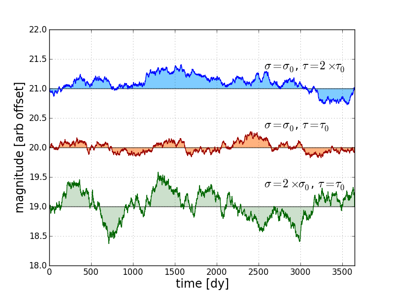
Figure 1.— . Examples of quasar light curves generated by the CAR model, with different variability amplitude $\sigma$ and characteristic time-scale $\tau$ ($\sigma_{0}=0.01$ mag day^-1/2 and $\tau_{0}=300$ day in this example).

The optical light curves of quasars arise from fluctuations in the brightness of the accretion disk with structure in the time series on the order of days. Since these fluctuations are coherent, the implication is that the size of the accretion disk is roughly $R_{\rm src}\sim 10^{16}$ cm (which will be important for the microlensing calculation in Section 2.5). These fluctuations have been found to be well described by a damped random walk (DRW) stochastic process (see e.g.  Kelly et al., 2009; MacLeod et al., 2010; Zu et al., 2013). Initially, Kelly et al. (2009) introduced the Continuous Auto Regressive (CAR) process for fitting quasar light curves; this is equivalent to a Gaussian Process in which the covariance between two points on the light curve decreases as a function of their temporal separation. The CAR process is given by (see the Appendix in Kelly et al., 2009),

$$M(t)=e^{-t/\tau}M(0)+\bar{M}(1-e^{-t/\tau})+\sigma\int_{0}^{t}e^{-(t-s)/\tau}dB(s),$$ (2)

where $M$ is the magnitude of an image, $\tau$ is a characteristic timescale in days, $\bar{M}$ is the mean magnitude of the light curve in the absence of fluctuations, and $\sigma$ is the characteristic amplitude of the fluctuations in mag/day^1/2. In this model, fluctuations are generated by the integral term where $dB(s)$ is a normally distributed value with mean zero and variance $dt$. By fitting the above model to some 100 MACHO project light curves, Kelly et al. (2009) generated a distribution of $\tau$ and $\sigma$ for the MACHO quasars; we show typical examples of the CAR process with reasonable values for those parameters in Figure 1. Likewise, MacLeod et al. (2010) fit the DRW model to over 9000 quasars in the SDSS Stripe 82 region, again finding it to be a good description of the data, and exploring correlations between $\tau$ and $\sigma$, and quasar luminosity and black hole mass.

While the DRW process provides a good description of the data obtained so far, it is not yet clear whether it will remain so for longer baseline, higher cadence, or multi-filter light curves. The different emission regions of an AGN (different parts of the accretion disk, broad and narrow line clouds, etc.) are likely to vary in different ways (Eigenbrod et al., 2008; Sluse et al., 2011, 2012), suggesting that linear combinations of stochastic processes could provide more accurate descriptions (Kelly et al., 2011). These subcomponents would likely need parameters drawn from different distributions to the one above, and the correlations between the processes may need to be taken into account as well. Nevertheless, the success of the CAR model to date makes it a reasonable place to begin when simulating LSST-like AGN light curves.

2.4. Multiple Imaging by a Foreground Galaxy

For a given lens system, the time delays between images can be as short as $\sim$1 day for close pairs of images to as long as $\sim$100s of days for images on opposite sides of the lensing galaxy. The magnitude of these time delays (as well as the other observables) depends on the redshifts of both the lens galaxy, $z_{l}$, and the source redshift, $z_{s}$, and therefore it is important to understand the expected distribution of those parameters in the LSST sample. Oguri & Marshall (2010, hereafter OM10) generated a mock catalog of LSST lensed AGN based on plausible models for the source quasars and lens galaxies, and simple assumptions for the detectability of lensed quasars, including published 10$\sigma$ limiting magnitude estimates, and the assumption that lenses will be detected if the third (second) brightest image for a given quad (double) is above this limit. This catalog provides a distribution of time delays that will be present in the LSST data which we can use to guide the generation of mock light curves.

Figure 2 shows the $\log_{10}\Delta t$ distributions for the OM10 double and quad sample. The distributions are roughly log-normal with means $\sim$10s of days and tails extending below 1 day for the quads, and above 100 days for the doubles. Lenses in both of these tails will have time delays that are difficult to measure, either because the cadence isn’t high enough, or because the observing seasons are not long enough. We expect some fraction of time delay measurements to fail catastrophically in these cases, but we also expect the catastrophe rate (and the robustness with which failure is reported) to vary with measurement algorithm.

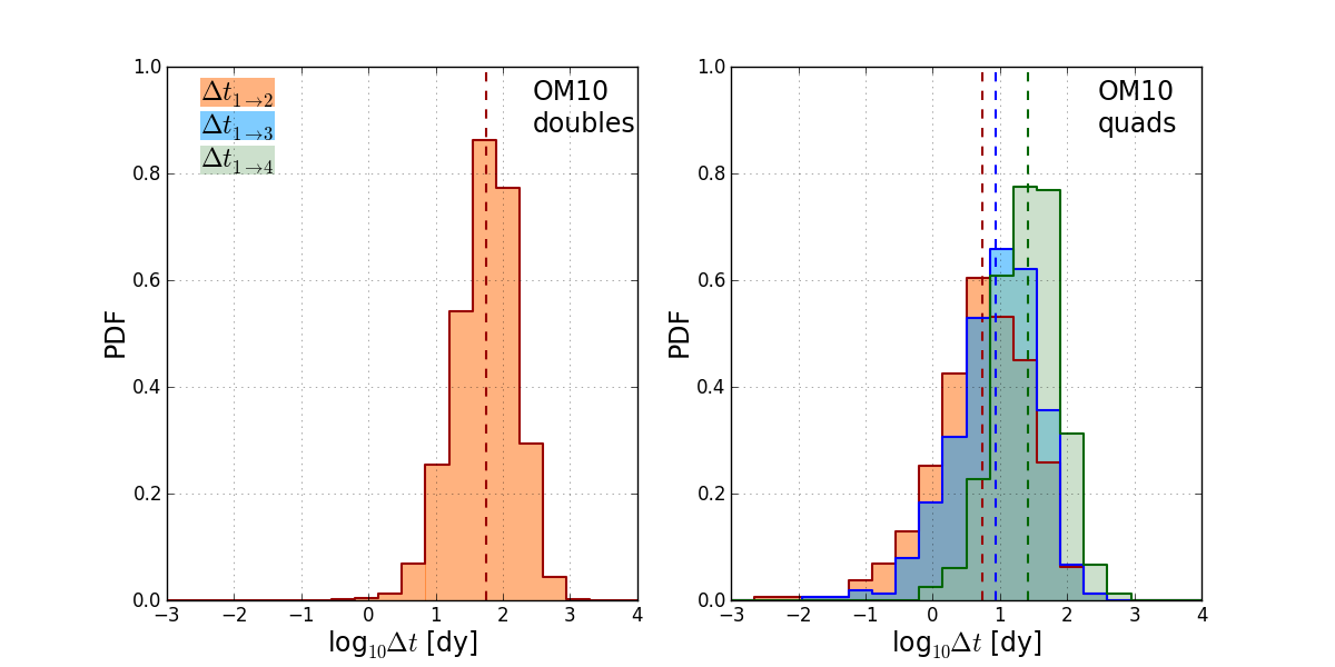
Figure 2.— The distribution of expected time delays in the OM10 mock lens catalog. Left: doubles, Right: quads. Dashed lines mark the means of the $\log_{10}\Delta t$ distributions.

2.5. Microlensing

As noted in Section 2.3, the physical size of a quasar accretion disk is $R_{\rm src}\sim 10^{15}$-$10^{16}$ cm, which, at cosmological distances, represents an angular size of $\sim 1$ $\mu$arcsecond ($\mu$as). In addition, the Einstein radius for a 1 $M_{\odot}$ point mass at these distances is also $\sim 1$ $\mu$as, indicating that the stars in the lens galaxy will typically have an order unity (or more) effect on the brightnesses of the individual images. Given the relevant angular scales, this phenomenon is termed “microlensing”.

Microlensing has long been acknowledged as a significant source of potential error when estimating time delays from optical monitoring data (see e.g. Schild, 1996; Schechter et al., 1997; Tewes et al., 2013a, and references therein) due to the fact that the relative velocity between the source and lens leads to time dependent fluctuations that are independent between the images. For caustic crossing events the relevant time scales are months to years, with smoother variations occurring over roughly decade timescales. As expected, the microlensing fluctuations are larger at bluer wavelengths, which correspond to smaller source sizes (e.g., Kochanek, 2004; Morgan et al., 2008). A solution to measuring time delays in the presence of these fluctuations (which are uncorrelated between the quasar images) is to model the microlensing in each image individually at the same time as inferring the time delay (e.g. Kochanek, 2004; Tewes et al., 2013b).

We create mock microlensing signals in each quasar image light curve by calculating the magnification as the source moves behind a static stellar field. The parameters involved are the local convergence, $\kappa$, and shear, $\gamma$, the fraction of surface density in stars, $F_{\star}$, the source size, $R_{\rm src}$, and the relative velocity between the quasar and the lens galaxy, $v_{\rm rel}$. We also include a Salpeter mass function for the stars though the amplitude of the fluctuations depends predominantly on the mean mass (which we take to be 1 $M_{\odot}$).

For each lens in the OM10 catalog we assign an $F_{\star}$ at each image position as follows. The OM10 catalog provides the velocity dispersion for a given lens which we use to estimate the $i$-band luminosity and effective radius of the galaxy by drawing from the Fundamental Plane (e.g.  Bernardi et al., 2003). For a given mass-to-light ratio, and assuming a standard de Vaucouleurs (1948) profile for the brightness distribution centered on the lens with an isothermal ellipsoid for the total mass distribution, we obtain the ratio of stellar mass density to total mass density, $F_{\star}$, at each image position.

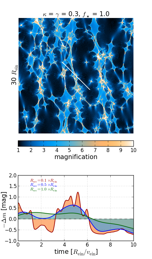
Figure 3.— Top: A typical source plane magnification map, showing the complex caustic structures caused by the stars in the lens galaxy. As the background quasar and foreground galaxy move relative to each other, the source traverses this pattern (white solid line), resulting in brightness fluctuations due to microlensing. Bottom: The fluctuations along this track (which traverses 10 stellar Einstein radii) are shown for three representative source sizes. Larger source sizes decrease the amplitude of the microlensing fluctuations as well as smooth out the shorter time scale features. Here “time” is given in units of Einstein radii crossing time (e.g., if the relative velocity between the lens and source is 1 $R_{\rm ein}$/yr [see text], then this track represents a 10 yr light curve.)

Given $\kappa$ and $\gamma$ from the OM10 catalog and estimating $F_{\star}$ as above, we generate magnification maps like the one shown in Figure 3, which represent the magnification of a point source as a function of position in the source plane. To use this map to generate temporal microlensing fluctuations, we first smooth it by a Gaussian source profile of appropriate size ($\sim 10^{15}$-$10^{16}$ cm) and then trace a linear path along a random direction in the map. This path is converted from source plane position to time units via a relative velocity $v_{\rm rel}$ (Kayser et al., 1986) which we compute from the velocities of matching galaxies drawn from the Millennium Survey. The effect of having a finite source is to smooth out and reduce the amplitude of the microlensing fluctuations.

2.6. Sampling

The current state-of-the-art lens monitoring campaign, COSMOGRAIL, typically visits each of its targets every few nights during each of several observing seasons each lasting many months. For example, Tewes et al. (2013b) present 9 seasons of monitoring for the lensed quasar RXJ1131$-$1231 where the mean season length was 7.7 months ($\pm 2$ weeks) and the median cadence was 3 days. These observations were taken in the same R-band filter, with considerable attention paid to photometric calibration and PSF estimation based on the surrounding star field. These data allowed Tewes et al. (2013b) to measure a time delay of 91 days to 1.5% precision.

While this quality of measurement is possible for small samples (a few tens) of lenses, the larger sample of lensed quasars lying in the LSST survey footprint will all be monitored over the course of its ten year campaign, but at lower cadence and with shorter seasons. In the simplest possible “universal cadence” observing strategy, we would expect the mean cadence to be around 4 days between visits, in any filter, and with some variation with time as the scheduler responds to the needs of the various science programs and the changing conditions; the gaps between observations in the same filter will tend to be longer (Ivezic et al., 2008; LSST Science Collaboration et al., 2009). The season length in this strategy is likely to be approximately 4 months (with variation among filters), in order to keep the telescope pointing at low airmass (see example in Figure 4). The primary impact of the shorter season length will be to make it hard to measure time delays of more than 100 days; the LSST universal cadence time delay lens sample would be biased towards delays shorter than this.

The universal cadence strategy may not turn out to be optimal, and we can explore various LSST observing strategies by simulating light curves with a range of cadences and season lengths. Shorter cadences and longer seasons are closer to those obtained by COSMOGRAIL. As its lens sample increases in size, blind analysis of the COSMOGRAIL datasets will provide an increasingly better understanding of the accuracy available to the program. We note that only if all filters’ light curves can be fitted simultaneously with a model for the multi-filter variability would the maximum, any-filter cadence be fully exploited. Even if that fitting is not possible, the dithered nature of the different filters’ light curves should still allow a time resolution approaching that of the any-filter cadence.

The remaining variables in the mock light curve generation pertain to the photometric uncertainties applied to the sampled fluxes. Tewes et al. (2013a) provide a summary of possible sources of uncertainty and error in the photometric measurements, which we follow in generating light curves with realistic uncertainties, including in the accuracy of the error reporting. The OM10 mock lens sample contains a variety of quasar image brightnesses, allowing us to investigate time delay accuracy as a function of signal to noise, or, for LSST, source magnitude. We note that for this first challenge, uncertainties arising from contamination by the light of the foreground source were not taken into account. Those might be important, especially for the fainter images and this should be addressed in future challenges.

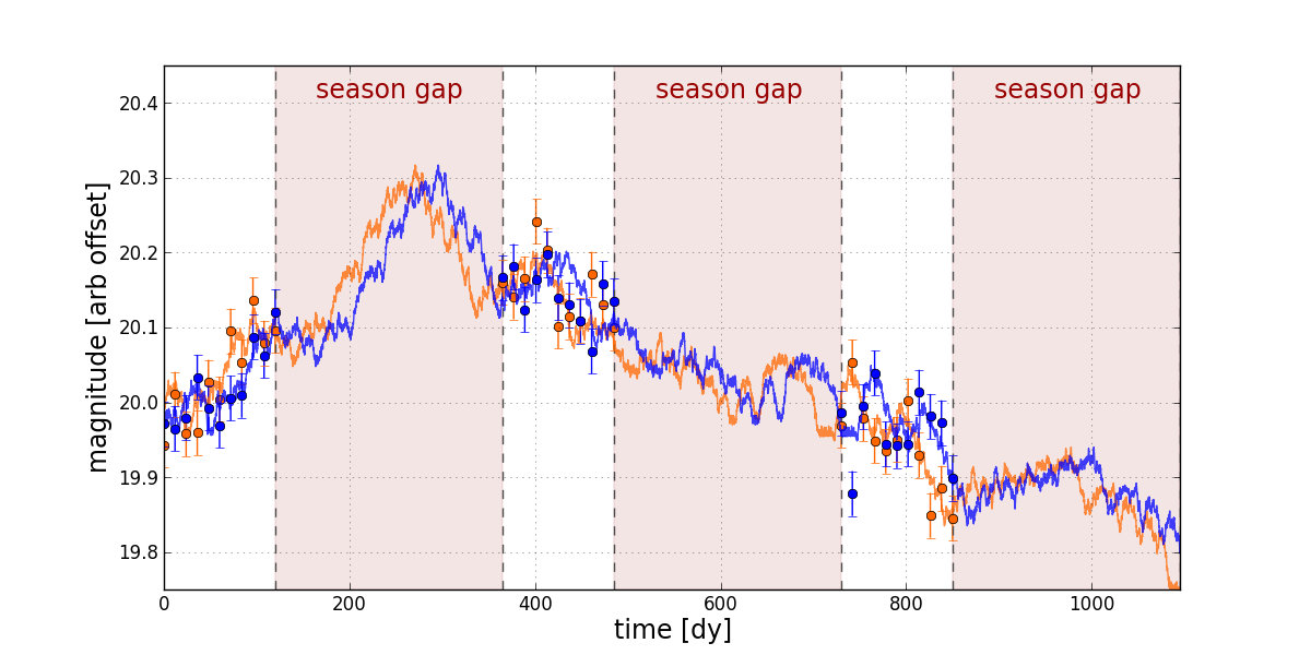
Figure 4.— Example light curves for a simulated double lensed quasar. The blue light curve lags behind the red light curve as a result of the gravitational time delay. The filled circles with error bars represent an actual mock observation in which noise and measurement uncertainty are added, while the finite season lengths lead to gaps in the data.

3. The Structure of the Challenge

This section outlines the two initial steps of the challenge, gives the instructions for participation and timeline, and defines the goal of the challenge and the criteria for evaluation.

3.1. The Challenge Ladders

The initial challenge consists of two parts, hereafter time delay challenge 0 and 1 (TDC0 and TDC1). Each of these is organized as a ladder with a number of simulated light curves at each rung. The rungs are intended to represent increasing levels of difficulty and realism within each challenge. The simulated light curves were created by the “evil” team (authors GD, CDF, KL, PJM, NR, and TT). All the details about the light curves, including input parameters, noise properties, etc., were only revealed to the participating teams (hereafter “good” teams) after the closing of the challenge.

TDC0 consists of a small number of simulated light curves with fairly basic properties in terms of noise, sampling season, and cadence. It is intended to serve as a validation tool before embarking on TDC1. The “evil” team expects that state of the art algorithms should be able to process TDC0 with minimal computing time and recover the input time delays within the estimated uncertainties. TDC0 also provides a means to perform basic debugging, and to test input and output formats for the challenge. The truth file for TDC0 will not be revealed until after the closing of TDC1 to preserve blindness.

TDC1 consists of thousands of sets of simulated light curves, also arranged in rungs of increasing difficulty and realism. The large data volume is chosen to simulate the demands of an LSST-like experiment, and to be able to detect biases in the algorithms at the sub-percent level. The “evil” team expects processing of the TDC1 dataset to be challenging with current algorithms in terms of computing resources. TDC1 thus represents a test of the accuracy of the algorithms but also of their efficiency. Incomplete submissions were accepted, although the number of processed light curves is one of the metrics by which algorithms were evaluated, as described below.

The mock data generated for the highest rungs of the initial challenge ladders TDC0 and TDC1 are as realistic as our current simulation technology allows, but lower rungs are somewhat simplified. This design is based on the successful weak lensing STEP (Heymans et al., 2006; Massey et al., 2007) and GREAT (Bridle et al., 2010; Kitching et al., 2013, 2012; Mandelbaum et al., 2013) shape estimation challenges, where the former tried to be as realistic as possible, while the latter focused on specific aspects of the problem. Still, following a successful outcome of TDC0 and TDC1 we anticipate in the future further increasing the complexity of the simulations so as to stimulate gradual improvements in the algorithms over the remainder of this decade. Our approach of testing on simulated data is very complementary to tests on real data. The former allow one to test blindly for accuracy but they are valid only insofar as the simulations are realistic, while the latter provide a valuable test of consistency (but not accuracy) on actual data, including all the unknown unknowns.

3.2. Instructions for participation, timeline, and ranking criteria

Instructions for how to access the simulated light curves in the time delay challenge are given at the challenge website. In short, participation in the challenge required the following steps.

3.2.1 TDC0

Every prospective “good” team was invited to download the TDC0 light curves and analyze them. Upon completion of the analysis, they were asked to submit their time delay estimates, together with their estimated 68% uncertainties, to the challenge organizers for analysis. The simulation team calculated a minimum of four standard metrics given this set of estimated time delays $\tilde{\Delta t}$ and uncertainties $\delta$. The first metric is efficiency, quantified as the fraction of light curves $f$ for which an estimate is obtained. Of course, this is not a sufficient requirement for success, as the estimate should also be accurate and have correctly estimated uncertainties. There might be instances where the data are ambiguous (e.g., if time delay falls into season gaps), in which case some methods will indicate failure while others will estimate very large uncertainties.

Therefore, we need to introduce a second metric to evaluate how realistic the error estimate is. For this, we use the goodness of fit of the estimates, quantified by the standard reduced $\chi^{2}$:

$$\chi^{2}=\frac{1}{fN}\sum_{i}\left(\frac{\tilde{\Delta t}_{i}-\Delta t_{i}}{\delta_{i}}\right)^{2}.$$ (3)

where $\Delta t_{i}$ are the true time delays defined positive in input.

The third metric is the claimed precision of the estimator, quantified as the average relative uncertainty per lens:

$$P=\frac{1}{fN}\sum_{i}\frac{\delta_{i}}{\Delta t_{i}}.$$ (4)

The fourth is the accuracy of the estimator, quantified by the average fractional residual per lens

$$A=\frac{1}{fN}\sum_{i}\frac{\tilde{\Delta t}_{i}-\Delta t_{i}}{\Delta t_{i}}.$$ (5)

The initial function of these metrics is to define a minimal performance threshold that must be passed, in order to guarantee meaningful results in TDC1. “Good” teams are given aggregated statistical feedback on their TDC0 efforts, from which they can decide whether to continue to TDC1. The criteria for passing the TDC0 test are as follows:

$$f>0.3$$ (6)

$$0.5<\chi^{2}<2$$ (7)

$$P<15\%$$ (8)

$$|A|<15\%$$ (9)

A failure rate of 70% is something like the borderline of acceptability for LSST (given the total number of lenses expected), and so can be used to define the efficiency threshold. The TDC0 lenses were selected to span the range of possible time delays, rather than being sampled from the OM10 distribution, and so we therefore expect a higher rate of catastrophic failure at this stage than in TDC1: 30% successes is a minimal bar to clear.

The factor of two half-ranges in reduced $\chi^{2}$ correspond approximately to fits that include approximately 95% of the $\chi^{2}$ probability distribution when $N=8$, i.e. the number of time delays in every rung of TDC0: fits outside this range likely have problems with the time delay estimates, or the estimation of their uncertainties, or both. Requiring an average precision and accuracy of better than 15% is a further minimal bar to clear.

Repeat submissions were accepted for teams to iterate their analyses. TDC0 remained blinded until the TDC1 deadline on 1 July 2014. Late TDC0 submissions were accepted, but those teams had less time to carry out TDC1.

Rung	Sampling	Season duration	Noise	Microlensing
0	1 dy	12 mon	0.03 uni	no
1	1 dy	4 mon	0.03 uni	no
2	1 dy	4 mon	opsimish	no
3	2 wk	12 mon	0.03 uni	no
4	2 wk	4 mon	0.03 uni	no
5	opsimish	4 mon	opsimish	no
6	opsimish	4 mon	opsimish	yes

Table 1Design for 7 rungs in TDC0. The opsimish for sampling is a Gaussian distribution with mean sampling 12 days and deviation 2 days while the opsimish for noise is 0.053 in nanomaggies with error 0.016

As of July 1 2014, the closing date of TDC1, 13 teams participated in TDC0, using 47 different algorithms. Of those teams, seven qualified for TDC1. A summary of the results is shown in Figure 5. The seven qualified teams are revealed in a companion paper, where their TDC1 submissions are analyzed.

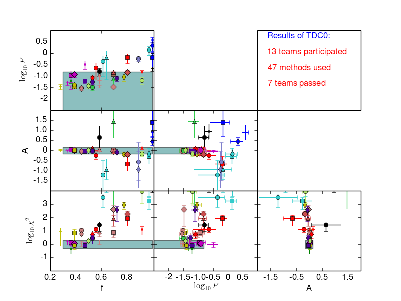
Figure 5.— Results of TDC0. Each color represents a different team, while each symbol represents a different method. The teams and methods are not identified to preserve confidentiality of the TDC0 submission.

3.2.2 TDC1

“Good” teams that successfully passed TDC0 and wished to continue were given access to the full TDC1. As in TDC0, the “good” teams estimated time delays and uncertainties and provided the answers to the “evil” team via a suitable web interface (found at the challenge website). The “evil” team computed the metrics described above. The results were not revealed until the end of the challenge in order to maintain blindness.

The deadline for TDC1 was 1 July 2014, seven months after that of TDC0. Multiple submissions were accepted from each team in order to allow for correction of bugs, and for different algorithms. However, only the first submission was considered blind. The most recent submission for each algorithm was also considered in order to allow for teams to improve their methods. Late submissions were accepted and included in the final publication if received in time but were flagged as such.

3.2.3 Publication of the results

Initially this first paper was only posted on the arXiv as a means to open the challenge. After the TDC1 deadline, this paper has been revised to include the details and results of TDC0. At the same time, the full details and results of TDC1 are described in the second paper of this series, including as co-authors all the members of the “good” teams who participated in the challenge. The two papers were submitted concurrently so as to allow the referee to evaluate the entire process. “Good” teams have been encouraged to publish papers on their own methods making use of the challenge data, if they felt they are presenting innovation worthy of publication.

3.3. Overall goals and broad criteria for success

The overall goal of TDC0 and TDC1 is to carry out a blind test of current state of the art time delay estimation algorithms in order to quantify the available accuracy. Criteria for success depend on the time horizon. At present, time delay cosmology is limited by the number of lenses with measured light curves and by the modeling uncertainties which are of order 5% per system (e.g., Suyu et al., 2010, 2013). Furthermore, distance measurements are currently in the range of accuracy of 3%. Therefore, any method that can currently provide time delays with realistic uncertainties ($\chi^{2}<1.5$) for the majority ($f>0.5$) of light curves with accuracy $A$ and precision $P$ better than 3% can be considered a competitive method.

In the longer run, with LSST in mind, a desirable goal is to maintain precision of $P<3\%$ per lens, but to improve the accuracy to $|A|<0.2\%$ in order for the sub-percent precision cosmological parameter estimates not to be limited by time delay measurement systematic biases. For $N=1000$, the 95% goodness of fit requirement becomes $\chi^{2}<1.09fN$, while keeping $f>0.5$. Testing for such extreme accuracy requires a large sample of lenses: TDC1 contains several thousand simulated systems to enable such tests.

4. Summary

Strong lens time delays are a powerful tool for cosmology. Like every cosmographic probe, in order to reach the precision and accuracy necessary to measure the dark energy equation of state it is essential to subject every component of the method to rigorous testing. With this motivation we have initiated a time delay challenge (TDC). In this paper, we have described the tools developed and used by the “evil team” to construct simulated light curves, laid out the structure of the challenge to the community, and given the results of TDC0.

The intrinsic quasar light curves are generated using a damped random walk process. The multiple images, flux ratios, and time delays are taken from the properties of a realistic simulated catalog of lenses expected for a survey like LSST. The effects of microlensing are computed using a newly developed fast code. Realistic noise and monitoring patterns are applied to the data. All simulation software is written in python and will be made publicly available after the completion of the challenge.

The challenge consists of two steps, TDC0, consisting of a few pairs of image light curves, intended to provide “good” teams with the opportunity to test and debug their codes before launching into the more computationally intensive TDC1. In total, 13 teams participated in TDC0 using 47 different methods. Seven of those teams qualified for TDC1. The TDC1 dataset consists of thousands of light curves, a number sufficient to identify biases at the subpercent level required for Stage IV experiments.

The challenge data are available to download at

http://timedelaychallenge.org

The deadlines for the challenges were December 1, 2013 for TDC0, and July 1, 2014 for TDC1. The challenge is (still) open to anyone. The results of TDC1 are published in a companion paper with all the participating teams as co-authors (Liao et al., 2014).

References

- Bernardi et al. (2003) Bernardi, M., Sheth, R. K., Annis, J., Burles, S., Eisenstein, D. J., Finkbeiner, D. P., Hogg, D. W., Lupton, R. H., Schlegel, D. J., SubbaRao, M., Bahcall, N. A., Blakeslee, J. P., Brinkmann, J., Castander, F. J., Connolly, A. J., Csabai, I., Doi, M., Fukugita, M., Frieman, J., Heckman, T., Hennessy, G. S., Ivezić, Ž., Knapp, G. R., Lamb, D. Q., McKay, T., Munn, J. A., Nichol, R., Okamura, S., Schneider, D. P., Thakar, A. R., & York, D. G. 2003, AJ, 125, 1866
- Biggs et al. (1999) Biggs, A. D., Browne, I. W. A., Helbig, P., Koopmans, L. V. E., Wilkinson, P. N., & Perley, R. A. 1999, MNRAS, 304, 349
- Bridle et al. (2010) Bridle, S., Balan, S. T., Bethge, M., Gentile, M., Harmeling, S., Heymans, C., Hirsch, M., Hosseini, R., Jarvis, M., Kirk, D., Kitching, T., Kuijken, K., Lewis, A., Paulin-Henriksson, S., Schölkopf, B., Velander, M., Voigt, L., Witherick, D., Amara, A., Bernstein, G., Courbin, F., Gill, M., Heavens, A., Mandelbaum, R., Massey, R., Moghaddam, B., Rassat, A., Réfrégier, A., Rhodes, J., Schrabback, T., Shawe-Taylor, J., Shmakova, M., van Waerbeke, L., & Wittman, D. 2010, MNRAS, 405, 2044
- Burud et al. (2002a) Burud, I., Courbin, F., Magain, P., Lidman, C., Hutsemékers, D., Kneib, J.-P., Hjorth, J., Brewer, J., Pompei, E., Germany, L., Pritchard, J., Jaunsen, A. O., Letawe, G., & Meylan, G. 2002a, A&A, 383, 71
- Burud et al. (2002b) —. 2002b, A&A, 383, 71
- Burud et al. (2002c) Burud, I., Hjorth, J., Courbin, F., Cohen, J. G., Magain, P., Jaunsen, A. O., Kaas, A. A., Faure, C., & Letawe, G. 2002c, A&A, 391, 481
- de Vaucouleurs (1948) de Vaucouleurs, G. 1948, Annales d’Astrophysique, 11, 247
- Eigenbrod et al. (2008) Eigenbrod, A., Courbin, F., Sluse, D., Meylan, G., & Agol, E. 2008, A&A, 480, 647
- Eulaers et al. (2013) Eulaers, E., Tewes, M., Magain, P., Courbin, F., Asfandiyarov, I., Ehgamberdiev, S., Rathna Kumar, S., Stalin, C. S., Prabhu, T. P., Meylan, G., & Van Winckel, H. 2013, A&A, 553, A121
- Fassnacht et al. (1999) Fassnacht, C. D., Pearson, T. J., Readhead, A. C. S., Browne, I. W. A., Koopmans, L. V. E., Myers, S. T., & Wilkinson, P. N. 1999, ApJ, 527, 498
- Fassnacht et al. (2002) Fassnacht, C. D., Xanthopoulos, E., Koopmans, L. V. E., & Rusin, D. 2002, ApJ, 581, 823
- Goicoechea et al. (2008) Goicoechea, L. J., Shalyapin, V. N., Koptelova, E., Gil-Merino, R., Zheleznyak, A. P., & Ullán, A. 2008, Nature, 13, 182
- Heymans et al. (2006) Heymans, C., Van Waerbeke, L., Bacon, D., Berge, J., Bernstein, G., Bertin, E., Bridle, S., Brown, M. L., Clowe, D., Dahle, H., Erben, T., Gray, M., Hetterscheidt, M., Hoekstra, H., Hudelot, P., Jarvis, M., Kuijken, K., Margoniner, V., Massey, R., Mellier, Y., Nakajima, R., Refregier, A., Rhodes, J., Schrabback, T., & Wittman, D. 2006, MNRAS, 368, 1323
- Hojjati et al. (2013) Hojjati, A., Kim, A. G., & Linder, E. V. 2013, Phys. Rev. D, 87, 123512
- Ivezic et al. (2008) Ivezic, Z., Tyson, J. A., Acosta, E., Allsman, R., Anderson, S. F., Andrew, J., Angel, R., Axelrod, T., Barr, J. D., Becker, A. C., Becla, J., Beldica, C., Blandford, R. D., Bloom, J. S., Borne, K., Brandt, W. N., Brown, M. E., Bullock, J. S., Burke, D. L., Chandrasekharan, S., Chesley, S., Claver, C. F., Connolly, A., Cook, K. H., Cooray, A., Covey, K. R., Cribbs, C., Cutri, R., Daues, G., Delgado, F., Ferguson, H., Gawiser, E., Geary, J. C., Gee, P., Geha, M., Gibson, R. R., Gilmore, D. K., Gressler, W. J., Hogan, C., Huffer, M. E., Jacoby, S. H., Jain, B., Jernigan, J. G., Jones, R. L., Juric, M., Kahn, S. M., Kalirai, J. S., Kantor, J. P., Kessler, R., Kirkby, D., Knox, L., Krabbendam, V. L., Krughoff, S., Kulkarni, S., Lambert, R., Levine, D., Liang, M., Lim, K., Lupton, R. H., Marshall, P., Marshall, S., May, M., Miller, M., Mills, D. J., Monet, D. G., Neill, D. R., Nordby, M., O’Connor, P., Oliver, J., Olivier, S. S., Olsen, K., Owen, R. E., Peterson, J. R., Petry, C. E., Pierfederici, F., Pietrowicz, S., Pike, R., Pinto, P. A., Plante, R., Radeka, V., Rasmussen, A., Ridgway, S. T., Rosing, W., Saha, A., Schalk, T. L., Schindler, R. H., Schneider, D. P., Schumacher, G., Sebag, J., Seppala, L. G., Shipsey, I., Silvestri, N., Smith, J. A., Smith, R. C., Strauss, M. A., Stubbs, C. W., Sweeney, D., Szalay, A., Thaler, J. J., Vanden Berk, D., Walkowicz, L., Warner, M., Willman, B., Wittman, D., Wolff, S. C., Wood-Vasey, W. M., Yoachim, P., Zhan, H., & for the LSST Collaboration. 2008, ArXiv e-prints
- Kayser et al. (1986) Kayser, R., Refsdal, S., & Stabell, R. 1986, A&A, 166, 36
- Keeton & Moustakas (2009) Keeton, C. R., & Moustakas, L. A. 2009, ApJ, 699, 1720
- Kelly et al. (2009) Kelly, B. C., Bechtold, J., & Siemiginowska, A. 2009, ApJ, 698, 895
- Kelly et al. (2011) Kelly, B. C., Sobolewska, M., & Siemiginowska, A. 2011, ApJ, 730, 52
- Kitching et al. (2012) Kitching, T. D., Balan, S. T., Bridle, S., Cantale, N., Courbin, F., Eifler, T., Gentile, M., Gill, M. S. S., Harmeling, S., Heymans, C., Hirsch, M., Honscheid, K., Kacprzak, T., Kirkby, D., Margala, D., Massey, R. J., Melchior, P., Nurbaeva, G., Patton, K., Rhodes, J., Rowe, B. T. P., Taylor, A. N., Tewes, M., Viola, M., Witherick, D., Voigt, L., Young, J., & Zuntz, J. 2012, MNRAS, 423, 3163
- Kitching et al. (2013) Kitching, T. D., Rowe, B., Gill, M., Heymans, C., Massey, R., Witherick, D., Courbin, F., Georgatzis, K., Gentile, M., Gruen, D., Kilbinger, M., Li, G. L., Mariglis, A. P., Meylan, G., Storkey, A., & Xin, B. 2013, ApJS, 205, 12
- Kochanek (2004) Kochanek, C. S. 2004, ApJ, 605, 58
- Kochanek et al. (2006) Kochanek, C. S., Morgan, N. D., Falco, E. E., McLeod, B. A., Winn, J. N., Dembicky, J., & Ketzeback, B. 2006, ApJ, 640, 47
- Kundic et al. (1995) Kundic, T., Colley, W. N., Gott, III, J. R., Malhotra, S., Pen, U.-L., Rhoads, J. E., Stanek, K. Z., Turner, E. L., & Wambsganss, J. 1995, ApJ, 455, L5
- Kundic et al. (1997) Kundic, T., Turner, E. L., Colley, W. N., Gott, III, J. R., Rhoads, J. E., Wang, Y., Bergeron, L. E., Gloria, K. A., Long, D. C., Malhotra, S., & Wambsganss, J. 1997, ApJ, 482, 75
- Liao et al. (2014) Liao, K., Treu, T., Marshall, P., Fassnacht, C. D., Rumbaugh, N., Dobler, G., Aghamousa, A., Bonvin, V., Courbin, F., Hojjati, A., Jackson, N., Kashyap, V., Rathna Kumar, S., Linder, E., Mandel, K., Meng, X.-L., Meylan, G., Moustakas, L. A., Prabhu, T. P., Romero-Wolf, A., Shafieloo, A., Siemiginowska, A., Stalin, C. S., Tak, H., Tewes, M., & van Dyk, D. 2014, arXiv:1409.1254
- Linder (2011) Linder, E. V. 2011, Phys. Rev. D, 84, 123529
- Lovell et al. (1998) Lovell, J. E. J., Jauncey, D. L., Reynolds, J. E., Wieringa, M. H., King, E. A., Tzioumis, A. K., McCulloch, P. M., & Edwards, P. G. 1998, ApJ, 508, L51
- LSST Science Collaboration et al. (2009) LSST Science Collaboration, Abell, P. A., Allison, J., Anderson, S. F., Andrew, J. R., Angel, J. R. P., Armus, L., Arnett, D., Asztalos, S. J., Axelrod, T. S., & et al. 2009, ArXiv e-prints
- MacLeod et al. (2010) MacLeod, C. L., Ivezić, Ž., Kochanek, C. S., Kozłowski, S., Kelly, B., Bullock, E., Kimball, A., Sesar, B., Westman, D., Brooks, K., Gibson, R., Becker, A. C., & de Vries, W. H. 2010, ApJ, 721, 1014
- Magain et al. (1998) Magain, P., Courbin, F., & Sohy, S. 1998, ApJ, 494, 472
- Mandelbaum et al. (2013) Mandelbaum, R., Rowe, B., Bosch, J., Chang, C., Courbin, F., Gill, M., Jarvis, M., Kannawadi, A., Kacprzak, T., Lackner, C., Leauthaud, A., Miyatake, H., Nakajima, R., Rhodes, J., Simet, M., Zuntz, J., Armstrong, B., Bridle, S., Coupon, J., Dietrich, J. P., Gentile, M., Heymans, C., Jurling, A. S., Kent, S. M., Kirkby, D., Margala, D., Massey, R., Melchior, P., Peterson, J., Roodman, A., & Schrabback, T. 2013, ArXiv e-prints
- Massey et al. (2007) Massey, R., Heymans, C., Bergé, J., Bernstein, G., Bridle, S., Clowe, D., Dahle, H., Ellis, R., Erben, T., Hetterscheidt, M., High, F. W., Hirata, C., Hoekstra, H., Hudelot, P., Jarvis, M., Johnston, D., Kuijken, K., Margoniner, V., Mandelbaum, R., Mellier, Y., Nakajima, R., Paulin-Henriksson, S., Peeples, M., Roat, C., Refregier, A., Rhodes, J., Schrabback, T., Schirmer, M., Seljak, U., Semboloni, E., & van Waerbeke, L. 2007, MNRAS, 376, 13
- Morgan et al. (2008) Morgan, C. W., Kochanek, C. S., Dai, X., Morgan, N. D., & Falco, E. E. 2008, ApJ, 689, 755
- Oguri & Marshall (2010) Oguri, M., & Marshall, P. J. 2010, MNRAS, 405, 2579
- Paraficz & Hjorth (2009) Paraficz, D., & Hjorth, J. 2009, A&A, 507, L49
- Pelt et al. (1994) Pelt, J., Hoff, W., Kayser, R., Refsdal, S., & Schramm, T. 1994, A&A, 286, 775
- Pelt et al. (1996) Pelt, J., Kayser, R., Refsdal, S., & Schramm, T. 1996, A&A, 305, 97
- Press et al. (1992a) Press, W. H., Rybicki, G. B., & Hewitt, J. N. 1992a, ApJ, 385, 404
- Press et al. (1992b) —. 1992b, ApJ, 385, 416
- Rathna Kumar et al. (2013) Rathna Kumar, S., Tewes, M., Stalin, C. S., Courbin, F., Asfandiyarov, I., Meylan, G., Eulaers, E., Prabhu, T. P., Magain, P., Van Winckel, H., & Ehgamberdiev, S. 2013, ArXiv e-prints
- Refsdal (1964) Refsdal, S. 1964, MNRAS, 128, 307
- Schechter et al. (1997) Schechter, P. L., Bailyn, C. D., Barr, R., Barvainis, R., Becker, C. M., Bernstein, G. M., Blakeslee, J. P., Bus, S. J., Dressler, A., Falco, E. E., Fesen, R. A., Fischer, P., Gebhardt, K., Harmer, D., Hewitt, J. N., Hjorth, J., Hurt, T., Jaunsen, A. O., Mateo, M., Mehlert, D., Richstone, D. O., Sparke, L. S., Thorstensen, J. R., Tonry, J. L., Wegner, G., Willmarth, D. W., & Worthey, G. 1997, ApJ, 475, L85
- Schild (1996) Schild, R. E. 1996, ApJ, 464, 125
- Sluse et al. (2012) Sluse, D., Hutsemékers, D., Courbin, F., Meylan, G., & Wambsganss, J. 2012, A&A, 544, A62
- Sluse et al. (2011) Sluse, D., Schmidt, R., Courbin, F., Hutsemékers, D., Meylan, G., Eigenbrod, A., Anguita, T., Agol, E., & Wambsganss, J. 2011, A&A, 528, A100
- Suyu et al. (2013) Suyu, S. H., Auger, M. W., Hilbert, S., Marshall, P. J., Tewes, M., Treu, T., Fassnacht, C. D., Koopmans, L. V. E., Sluse, D., Blandford, R. D., Courbin, F., & Meylan, G. 2013, ApJ, 766, 70
- Suyu et al. (2010) Suyu, S. H., Marshall, P. J., Auger, M. W., Hilbert, S., Blandford, R. D., Koopmans, L. V. E., Fassnacht, C. D., & Treu, T. 2010, ApJ, 711, 201
- Tewes et al. (2013a) Tewes, M., Courbin, F., & Meylan, G. 2013a, A&A, 553, A120
- Tewes et al. (2013b) Tewes, M., Courbin, F., Meylan, G., Kochanek, C. S., Eulaers, E., Cantale, N., Mosquera, A. M., Magain, P., Van Winckel, H., Sluse, D., Cataldi, G., Vørøs, D., & Dye, S. 2013b, A&A, 556, A22
- Walsh et al. (1979) Walsh, D., Carswell, R. F., & Weymann, R. J. 1979, Nature, 279, 381
- Zu et al. (2013) Zu, Y., Kochanek, C. S., Kozłowski, S., & Udalski, A. 2013, ApJ, 765, 106