Molecular branch of a small highly-elongated Fermi gas with an impurity: Full three-dimensional versus effective one-dimensional description

Abstract

We consider an impurity immersed in a small Fermi gas under highly-elongated harmonic confinement. The impurity interacts with the atoms of the Fermi gas through an isotropic short-range potential with three-dimensional free-space $s$-wave scattering length $a_{3\text{d}}$. We investigate the energies of the molecular branch, i.e., the energies of the state that corresponds to a gas consisting of a weakly-bound diatomic molecule and “unpaired” atoms, as a function of the $s$-wave scattering length $a_{3\text{d}}$ and the ratio $\eta$ between the angular trapping frequencies in the tight and weak confinement directions. The energies obtained from our three-dimensional description that accounts for the dynamics in the weak and tight confinement directions are compared with those obtained within an effective one-dimensional framework, which accounts for the dynamics in the tight confinement direction via a renormalized one-dimensional coupling constant. Our theoretical results are related to recent experimental measurements.

I Introduction

Ultracold few-atom systems provide clean model systems in which the system parameters such as the interaction strength and confinement geometry can be controlled with high accuracy BlumeReview ; GiorginiReview ; BlochReview ; ChinReview . Recently, two-component Fermi gases consisting of lithium atoms in two different hyperfine states have been prepared and probed experimentally in highly elongated, nearly harmonic external traps with an aspect ratio $\eta$ around ten Jochim1 ; Jochim2 ; sala13 ; Jochim3 ; Jochim4 ; thesisGerhard . In two-component ⁶Li mixtures, the interspecies $s$-wave scattering length $a_{3\text{d}}$ can be tuned by varying an external magnetic field in the vicinity of a Fano-Feshbach resonance ChinReview . The intraspecies interactions are, to a very good approximation, negligible since the experiments operate at field strengths that are quite far away from $p$-wave and higher partial wave resonances. Thus, since the harmonic oscillator lengths $a_{\rho}$ and $a_{z}$ that characterize the confinement in the tight and weak confinement directions are much larger than the van der Waals length $r_{\text{vdW}}$ of the lithium-lithium potential, the system dynamics is, to a very good approximation, governed by the $s$-wave scattering length $a_{3\text{d}}$, the aspect ratio $\eta$ and the numbers $N_{1}$ and $N_{2}$ of fermions in the first and the second component, respectively.

This paper investigates the energetics of a single impurity immersed in a gas of fermions, referred to as the $(N-1,1)$ system, where $N$ denotes the total number of particles. We focus on small systems with $N=2-4$ and determine the energy of the molecular branch. This is the branch that can be populated by preparing the system in the non-interacting regime, i.e., with vanishing interspecies $s$-wave scattering length, and by adiabatically tuning the external magnetic field such that the $s$-wave scattering length takes small negative to infinitely large to positive values. Since equal-mass two-component Fermi gases with short-range $s$-wave interactions do only support weakly-bound dimers and not weakly-bound trimers or tetramers BlumeReview , the molecular branch consists, roughly speaking, of a diatomic molecule that interacts with the “unpaired” atoms. This work compares the energies obtained from a full three-dimensional treatment and an effective one-dimensional treatment. The latter is expected to break down when the size of the dimer becomes comparable to the harmonic oscillator length $a_{\rho}$ of the tight confinement direction. This is the regime where the system is expected to “explicitly feel” the degrees of freedom associated with the tight confinement direction. Assuming harmonic confinement, we provide quantitative comparisons of the full three-dimensional and approximate one-dimensional treatments as a function of the $s$-wave scattering length and the aspect ratio $\eta$. We compare our energies of the molecular branch to those determined experimentally via radio frequency spectroscopy Jochim3 ; thesisGerhard . While the dynamics of the molecular branch of the $(1,1)$ system has been investigated extensively in the literature bolda03 ; Idziaszek05 ; Idziaszek06 ; sala13 , that of the $(2,1)$ and $(3,1)$ systems has not yet been investigated comprehensively theoretically although first steps have been taken mora05 ; mora05a .

A full quantitative theoretical understanding of the energetics of the molecular branch of small Fermi gases under highly-elongated confinement is important for several reasons. Experiments on few-fermion systems are becoming more and more precise Jochim5 ; sala13 , opening the door for quantitative studies of a myriad of few-atom phenomena. Moreover, a thorough understanding of few-body systems serves as a guide for larger systems where the analysis relies, in many cases, on approximate treatments and plays a crucial ingredient in mapping out the transition from few- to many-body physics Jochim4 ; Jochim3 ; thesisGerhard .

The remainder of this paper is organized as follows. Section II introduces the system Hamiltonian and reviews briefly how to solve the corresponding time-independent Schrödinger equation. Section III presents our results for the full three-dimensional and the approximate one-dimensional treatments. Lastly, Sec. IV summarizes.

II System Hamiltonian

The three-dimensional system Hamiltonian $H_{3\text{d}}$ for the $N$ fermions of mass $m$ reads

$$H_{3\text{d}}=\sum_{j=1}^{N}\left[\frac{-\hbar^{2}}{2m}\nabla_{\vec{r}_{j}}^{2}+\frac{1}{2}m\left(\omega_{\rho}^{2}\rho_{j}^{2}+\omega_{z}^{2}z_{j}^{2}\right)\right]+$$

$$\sum_{j=1}^{N_{1}}\sum_{k=N_{1}+1}^{N}V_{\text{tb}}(\vec{r}_{jk}),$$ (1)

where $\vec{r}_{j}$ denotes the position vector of the $j$th atom measured with respect to the trap center, $\vec{r}_{j}=(x_{j},y_{j},z_{j})$, and $\rho_{j}^{2}=x_{j}^{2}+y_{j}^{2}$. The angular trapping frequencies $\omega_{\rho}$ and $\omega_{z}$ are related through the aspect ratio $\eta$, where $\eta=\omega_{\rho}/\omega_{z}$. Throughout, we consider elongated confining geometries with $\eta>1$ ($\eta=2,3,\cdots$). The interaction potential $V_{\text{tb}}(\vec{r}_{jk})$ between the unlike fermions is modeled by two different potentials, the regularized zero-range Fermi-Huang pseudopotential $V_{\text{ps}}(\vec{r}_{jk})$ ferm34 ; Huang57 ; HuangText ,

$$V_{\text{ps}}(\vec{r}_{jk})=\frac{4\pi\hbar^{2}a_{3\text{d}}}{m}\delta^{(3)}(\vec{r}_{jk})\frac{\partial}{\partial r_{jk}}r_{jk},$$ (2)

and a finite-range Gaussian potential $V_{\text{g}}(\vec{r}_{jk})$ with depth $V_{0}$ ($V_{0}\geq 0$) and range $r_{0}$,

$$V_{\text{g}}(\vec{r}_{jk})=-V_{0}\exp\left[-\left(\frac{r_{jk}}{\sqrt{2}r_{0}}\right)^{2}\right],$$ (3)

where $\vec{r}_{jk}=\vec{r}_{j}-\vec{r}_{k}$ and $r_{jk}=|\vec{r}_{jk}|$. In Eq. (2), $a_{3\text{d}}$ denotes the three-dimensional free-space zero-energy $s$-wave scattering length. To compare the eigenenergies of $H_{3\text{d}}$ for $V_{\text{ps}}$ and $V_{\text{g}}$, the depth $V_{0}$ and range $r_{0}$ are adjusted such that the free-space scattering lengths of the two potentials agree. Throughout, we restrict ourselves to the regime where $V_{\text{g}}$ supports zero free-space $s$-wave bound states for $a_{3\text{d}}<0$ and one free-space $s$-wave bound state for $a_{3\text{d}}>0$. We are interested in the regime where the range $r_{0}$ is much smaller than the oscillator lengths $a_{\rho}$ and $a_{z}$, where $a_{\rho}=\sqrt{\hbar/(m\omega_{\rho})}$ and $a_{z}=\sqrt{\hbar/(m\omega_{z})}$.

For sufficiently large $\eta$, the low-energy physics described by the three-dimensional Hamiltonian $H_{3\text{d}}$ is expected to be reproduced by the effective one-dimensional Hamiltonian $H_{1\text{d}}$ Olsh98 ,

$$H_{1\text{d}}=\sum_{j=1}^{N}\left(\frac{-\hbar^{2}}{2m}\frac{\partial^{2}}{\partial z_{j}^{2}}+\frac{1}{2}m\omega_{z}^{2}z_{j}^{2}\right)+$$

$$\sum_{j=1}^{N_{1}}\sum_{k=N_{1}+1}^{N}g_{1\text{d}}\delta^{(1)}(z_{jk})+N\hbar\omega_{\rho},$$ (4)

where $z_{jk}=z_{j}-z_{k}$. The effective one-dimensional coupling constant $g_{1\text{d}}$ Olsh98 ,

$$\frac{g_{1\text{d}}}{\hbar\omega_{\rho}\;a_{\rho}}=\frac{2a_{3\text{d}}}{a_{\rho}}\left(1+\frac{\zeta(1/2)}{\sqrt{2}}\frac{a_{3\text{d}}}{a_{\rho}}\right)^{-1}$$ (5)

with $\zeta(1/2)\approx-1.46035$, has been derived by analyzing $H_{3\text{d}}$ with $\omega_{z}=0$ for two particles with zero-range interactions. The renormalization of the one-dimensional coupling constant, i.e., the second term in the round brackets on the right hand side of Eq. (5), accounts for the occupation of excited transverse modes during the collision process (i.e., for virtual excitations). An improved description is obtained if the effective one-dimensional coupling constant is made to depend explicitly on the energy olshanii2 ; granger (see Sec. III for more details). It has been shown that the eigenenergies of the lowest gas-like state of $H_{1\text{d}}$ are in good agreement with those of $H_{3\text{d}}$ if the aspect ratio is sufficiently large Idziaszek06 ; Gharashi12 ; debraj . More specifically, the energy spacing $\hbar\omega_{\rho}$ in the tight confinement direction has to be larger than $(N_{1}-1)\hbar\omega_{z}$. This paper investigates the properties of the molecular branch for $H_{3\text{d}}$ and $H_{1\text{d}}$, i.e., we primarily focus on the regime where the eigenenergies are smaller than the ground state energy of the non-interacting Hamiltonian.

To determine the eigenstates and eigenenergies of $H_{3\text{d}}$ and $H_{1\text{d}}$, we separate the center of mass and relative degrees of freedom. The relative Schrödinger equation for the one-dimensional $(1,1)$, $(2,1)$ and $(3,1)$ systems is solved using the approaches introduced in Ref. Busch98 , Ref. Gharashi12 and Ref. Gharashi13 , respectively. The relative Schrödinger equation for the three-dimensional $(1,1)$ and $(2,1)$ systems interacting through $V_{\text{ps}}$ is solved using the approaches introduced in Ref. Idziaszek06 and Ref. Gharashi12 , respectively. For the $(3,1)$ system, we only consider the finite-range interaction model $V_{g}$. The relative Schrödinger equation for the three-dimensional $(1,1)$ system with finite-range interactions is solved using a B-spline approach while that for the three-dimensional $(2,1)$ and $(3,1)$ systems is solved using an explicitly correlated basis set expansion approach CGReview ; CGbook . For a fixed $a_{3\text{d}}$, we perform calculations for several $r_{0}$ and then extrapolate to the zero-range limit. Since the center of mass motion is uneffected by the two-body interactions, Sec. III reports the relative eigenenergies $E_{N_{1},N_{2}}^{\text{3d}}$ and $E_{N_{1},N_{2}}^{\text{1d}}$.

III Results

This section discusses the eigenenergies of the $(1,1)$, $(2,1)$ and $(3,1)$ systems. Squares in Fig. 1 show the relative zero-range energies $E_{N_{1},N_{2}}^{\text{3d}}$ of the energetically lowest lying molecular branch and the energetically lowest lying gaslike state as a function of $-1/g_{1\text{d}}$ for $\eta=10$. To make this plot, the three-dimensional scattering length $a_{3\text{d}}$ was converted to the effective one-dimensional coupling constant $g_{1\text{d}}$ using Eq. (5).

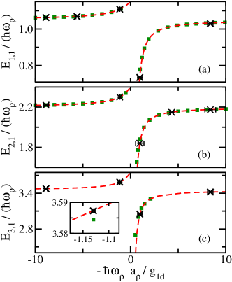
Figure 1: (Color online) Relative zero-range energies $E_{N_{1},N_{2}}$ as a function of $-1/g_{1\text{d}}$ for $\eta=10$. Squares and dashed lines show the relative energies obtained from the full three-dimensional treatment and the effective one-dimensional treatment, respectively, for (a) the $(1,1)$ system, (b) the $(2,1)$ system, and (c) the $(3,1)$ system. Crosses with errorbars show experimental results (the experimental data points are taken from Figure A.21. of Ref. thesisGerhard ). The inset in panel (c) shows a blow-up of the energetically lowest lying gas-like branch with negative $-g_{\text{1d}}$.

The non-interacting limit is reached for $-1/g_{1\text{d}}=\pm\infty$ and the infinitely strongly interacting regime for $|1/g_{1\text{d}}|=0$. The points $-1/g_{1\text{d}}=\pm\infty$ correspond to $a_{3\text{d}}=\mp 0$ while the point $|1/g_{1\text{d}}|=0$ corresponds to $a_{3\text{d}}=\sqrt{2}a_{\rho}/|\zeta(1/2)|$. The eigenstates corresponding to the relative eigenenergies of the $(1,1)$ system shown in Fig. 1(a) are characterized by an even parity in $z$, i.e., $\Pi_{z}=+1$, and vanishing projection quantum number $M$ and positive parity $\Pi_{\hat{\rho}}$ in the $xy$-plane explain_parity . The eigenstates corresponding to the relative eigenenergies of the $(2,1)$ and $(3,1)$ systems shown in Figs. 1(b) and 1(c), in contrast, are characterized by $(\Pi_{z},M,\Pi_{\hat{\rho}})=(-1,0,+1)$. The negative parity in the $z$-direction is a consequence of the fact that the majority particles have to obey the Pauli exclusion principle and that the single particle harmonic oscillator states in one dimension have alternating even and odd parity (even parity for the principal quantum numbers $n_{z}=0,2,\cdots$ and odd parity for the principal quantum numbers $n_{z}=1,3,\cdots$).

For comparison, dashed lines show the relative energies obtained within the one-dimensional framework. The agreement between the three- and one-dimensional energies of the energetically lowest lying gaslike branch is excellent (i.e., better than about $0.5$%) for all interaction strengths considered. For the $(1,1)$ and $(2,1)$ systems, quantitative comparisons have been presented in Refs. Idziaszek06 ; Gharashi12 . Figure 1(c) shows the three-dimensional energies of the energetically lowest lying gas-like state of the $(3,1)$ system for one $g_{1\text{d}}$ value, namely for $g_{1\text{d}}=0.8850\hbar\omega_{\rho}a_{\rho}$ [see inset of Fig. 1(c)]. We choose this value since this is one of the coupling strengths at which the experiments of the Heidelberg group were performed Jochim3 ; thesisGerhard . Our three-dimensional zero-range energy agrees with the corresponding one-dimensional energy to $0.1$%. The eigenenergies deduced from radio frequency spectroscopy measurements thesisGerhard are shown by crosses with errorbars. The experimental data have been, using theoretical three- and one-dimensional energies for the $(1,1)$ and $(2,1)$ systems Jochim3 ; thesisGerhard , converted to one-dimensional energies and should be considered as aproximations to the relative eigenenergies of $H_{1\text{d}}$. The agreement between the theoretical results and the energies deduced from experiment is at the few percent level, underlining the precision and control of modern cold atom experiments and the need for accurate theoretical treatments.

For the energetically lowest lying molecular branch of the $(1,1)$, $(2,1)$ and $(3,1)$ systems, the agreement between the three-dimensional energies (squares) and the one-dimensional energies (dashed lines) is excellent for large positive $-1/g_{1\text{d}}$ but deteriorates as $-1/g_{1\text{d}}$ decreases (see also Fig. 2). Qualitatively, this can be understood by realizing that the loosely bound dimer is very large for very positive $-1/g_{1\text{d}}$. In fact, the size of the loosely bound dimer is directly proportional to $|1/g_{1\text{d}}|$ Busch98 ; Olsh98 ; olshanii2 . As $-1/g_{1\text{d}}$ decreases and approaches zero, the size of the dimer decreases, implying that the system dynamics is no longer effectively one-dimensional but that the dimer is sufficiently small to “probe” the dynamics associated with the tight confinement direction. Since three- and higher-body bound states are absent, this qualitative argument applies not only to the $(1,1)$ system but also to the $(2,1)$ and $(3,1)$ systems. The experimental data for the molecular branch (see Fig. 1) are limited to fairly large $-1/g_{1\text{d}}$ and the errorbars are not small enough to discriminate between the three- and one-dimensional frameworks.

To quantify the applicability of the one-dimensional treatment for the molecular branch, we define the scaled interaction energy difference $\epsilon$,

$$\epsilon=\frac{E_{N-1,1}^{3\text{d,int}}-E_{N-1,1}^{1\text{d,int}}}{|E_{N-1,1}^{3\text{d,int}}|},$$ (6)

where $E_{N-1,1}^{3\text{d,int}}$ is defined as the difference between the relative three-dimensional energy $E_{N-1,1}^{\text{3d}}$ of the molecular branch and the non-interacting ground state energy, $E_{N-1,1}^{3\text{d,int}}=E_{N-1,1}^{\text{3d}}-E_{N-1,1}^{\text{NI}}$, where $E_{N-1,1}^{\text{NI}}=(N-1)^{2}\hbar\omega_{z}/2+(N-1)\hbar\omega_{\rho}$. The interaction energy $E_{N-1,1}^{1\text{d,int}}$ obtained from the one-dimensional treatment is defined in an analogous way (note that the non-interacting ground state energies of $H_{3\text{d}}$ and $H_{1\text{d}}$ are identical). Figure 2 shows the quantity $\epsilon$ as a function of $-1/g_{1\text{d}}$ for $\eta=10$. To determine $\epsilon$, we use the three-dimensional energies in the limit of zero-range interactions. The axis label on the top shows the one-dimensional scattering length $a_{1\text{d}}$, which is related to the one-dimensional coupling constant $g_{1\text{d}}$ via $a_{1\text{d}}=-2\hbar^{2}/(mg_{1\text{d}})$. Both $E_{N-1,1}^{3\text{d,int}}$ and $E_{N-1,1}^{1\text{d,int}}$ are negative. The quantity $\epsilon$ is small and negative for large $a_{\text{1d}}$ (see inset of Fig. 2) and changes sign around $a_{\text{1d}}\approx 5-10a_{\rho}$. The positive value of $\epsilon$ for $a_{\text{1d}}\lesssim 5-10a_{\rho}$ indicates that the energy obtained from the three-dimensional treatment lies above the energy obtained from the one-dimensional treatment.

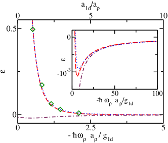
Figure 2: (Color online) Scaled interaction energy difference $\epsilon$ for the energetically lowest lying molecular branch as a function of $-1/g_{1\text{d}}$ for $\eta=10$. The dashed line, dotted line and diamonds show $\epsilon$ for the $(1,1)$, $(2,1)$ and $(3,1)$ systems, respectively; in these calculations, the interaction energy $E_{N-1,1}^{1\text{d},\text{int}}$ is calculated using $g_{1\text{d}}$. The dash-dotted line shows $\epsilon$ for the $(1,1)$ system for the case where the interaction energy $E_{N-1,1}^{1\text{d},\text{int}}$ is calculated using $g_{1\text{d}}^{\text{trap}}$, accounting for the energy-dependence of $\zeta(1/2,1-\epsilon_{2\text{b}}/2)$ but neglecting the “higher-order” Hurwitz zeta functions. The axis label on top shows the one-dimensional scattering length $a_{1\text{d}}$. The inset shows $\epsilon$ for large $-1/g_{\text{1d}}$.

When $a_{1\text{d}}$ is large, corresponding to a large dimer, the molecular branch is well described by the effective one-dimensional Hamiltonian. However, as $a_{1\text{d}}$ decreases and approaches $a_{\rho}$, the effective one-dimensional treatment deteriorates in a similar manner for the $(1,1)$, $(2,1)$ and $(3,1)$ systems. At $a_{1\text{d}}/a_{\rho}=1$, e.g., $\epsilon$ is equal to $0.55$, $0.55$ and $0.51$ for the $(1,1)$, $(2,1)$ and $(3,1)$ systems, respectively.

To better understand the behavior of $\epsilon$, we start with the implicit eigenequation for the three-dimensional $(1,1)$ system Idziaszek05 ; Idziaszek06 ,

$$\mathcal{F}_{3\text{d}}(\epsilon_{2\text{b}},\eta)=-\frac{\sqrt{2\eta}a_{\rho}}{a_{3\text{d}}},$$ (7)

where

$$\mathcal{F}_{3\text{d}}(\epsilon_{2\text{b}},\eta)=$$

$$\frac{1}{\sqrt{\pi}}\int_{0}^{\infty}\left(\frac{\eta e^{\eta\epsilon_{2\text{b}}t/2}}{\sqrt{1-e^{-t}}(1-e^{-\eta t})}-\frac{1}{t^{3/2}}\right)dt$$ (8)

and $\epsilon_{2\text{b}}=E_{1,1}^{3\text{d},\text{int}}/(\hbar\omega_{\rho})$. Equation (III) holds for $\epsilon_{2\text{b}}<0$ but can be extended to positive $\epsilon_{2\text{b}}$ through analytic continuation Idziaszek06 . To derive an effective one-dimensional eigenequation, we expand the integrand of Eq. (III), assuming small $1/\eta$, around $t=0$. Using this expansion in Eq. (7) yields

$$\frac{\Gamma(-\eta\epsilon_{2\text{b}}/2)}{\sqrt{2}\Gamma(-\eta\epsilon_{2\text{b}}/2+1/2)}=-\frac{2\hbar\omega_{\rho}a_{\rho}}{\sqrt{\eta}g_{1\text{d}}^{\text{trap}}},$$ (9)

where $g_{1\text{d}}^{\text{trap}}$ denotes the “trap-corrected” effective one-dimensional coupling constant,

$$\frac{g_{1\text{d}}^{\text{trap}}}{\hbar\omega_{\rho}a_{\rho}}=\frac{2a_{3\text{d}}}{a_{\rho}}\left\{1+\left[\frac{\zeta(1/2,1-\epsilon_{2\text{b}}/2)}{\sqrt{2}}+\frac{\zeta(3/2,1-\epsilon_{2\text{b}}/2)}{8\sqrt{2}\;\eta}+\frac{\zeta(5/2,1-\epsilon_{2\text{b}}/2)}{128\sqrt{2}\;\eta^{2}}+\dots\right]\frac{a_{3\text{d}}}{a_{\rho}}\right\}^{-1},$$ (10)

and $\zeta(\cdot,\cdot)$ the Hurwitz zeta function. If the series in Eq. (10) goes to sufficiently large order, the low-energy part of the eigenspectrum determined by solving Eq. (9) agrees very well with that determined by solving Eq. (7). It is important to note that Eq. (9) is the implicit eigenequation one obtains by solving the relative Schrödinger equation for the trapped two-particle system interacting through a zero-range potential with coupling constant $g_{1\text{d}}^{\text{trap}}$ Busch98 . Comparing the effective one-dimensional coupling constants $g_{1\text{d}}^{\text{trap}}$ and $g_{1\text{d}}$, we notice two things. First, the $\zeta(1/2)$ term in Eq. (5) is replaced by the energy-dependent Hurwitz zeta function. For small $|\epsilon_{2\text{b}}|$, the Hurwitz zeta function can be Taylor exanded, $\zeta(n/2,1-\epsilon_{2\text{b}}/2)\approx\zeta(n/2)+\zeta(1+n/2)n\epsilon_{2\text{b}}/4+\cdots$, showing that $\zeta(n/2,1-\epsilon_{2\text{b}}/2)$ reduces to $\zeta(1/2)$ for $\epsilon_{2\text{b}}=0$. Second, $g_{1\text{d}}^{\text{trap}}$ contains corrections that are suppressed by increasing powers of $1/\eta$ [the second and third terms in square brackets on the right hand side of Eq. (10)] and thus vanish as $\eta\rightarrow\infty$.

To see how the energy-dependence and the higher-order corrections in $1/\eta$ affect the energy spectrum of the $(1,1)$ system, we consider the weakly- and more strongly-interacting regimes separately. Expanding Eq. (9) around $\epsilon_{2\text{b}}=0$, we find

$$\frac{E_{1,1}^{1\text{d},\text{int}}}{\hbar\omega_{\rho}}=c_{1}^{(1)}\frac{g_{1\text{d}}^{\text{trap}}}{\hbar\omega_{\rho}a_{\rho}}+c_{1}^{(2)}\left(\frac{g_{1\text{d}}^{\text{trap}}}{\hbar\omega_{\rho}a_{\rho}}\right)^{2}+$$

$$c_{1}^{(3)}\left(\frac{g_{1\text{d}}^{\text{trap}}}{\hbar\omega_{\rho}a_{\rho}}\right)^{3}+\dots$$ (11)

or, rewriting this expression in terms of $g_{1\text{d}}$,

$$\frac{E_{1,1}^{1\text{d},\text{int}}}{\hbar\omega_{\rho}}=c_{1}^{(1)}\frac{g_{1\text{d}}}{\hbar\omega_{\rho}a_{\rho}}+(c_{1}^{(2)}+c_{2}^{(2)})\left(\frac{g_{1\text{d}}}{\hbar\omega_{\rho}a_{\rho}}\right)^{2}+$$

$$(c_{1}^{(3)}+c_{2}^{(3)}+c_{3}^{(3)})\left(\frac{g_{1\text{d}}}{\hbar\omega_{\rho}a_{\rho}}\right)^{3}+\dots.$$ (12)

The $c_{k}^{(j)}$-coefficients are listed in Table 1.

Table 1: Coefficients entering into Eqs. (III) and (III).

$c_{1}^{(1)}$	$\frac{1}{\sqrt{2\pi\eta}}$
$c_{1}^{(2)}$	$-\frac{\ln(2)}{2\pi}$
$c_{1}^{(3)}$	$\sqrt{\frac{\eta}{2\pi}}\left(-\frac{\pi}{48}+\frac{3\ln(2)^{2}}{4\pi}\right)$
$c_{2}^{(2)}$	$-\frac{c_{1}^{(1)}}{\sqrt{8}}\left(\frac{\zeta(3/2)}{2^{3}\eta}+\frac{\zeta(5/2)}{2^{7}\eta^{2}}+\dots\right)$
$c_{2}^{(3)}$	$\frac{-c_{1}^{(2)}}{\sqrt{2}}\left(\frac{\zeta(3/2)}{2^{3}\eta}+\frac{\zeta(5/2)}{2^{7}\eta^{2}}+\dots\right)+$
	$\frac{c_{1}^{(1)}}{8}\left(\frac{\zeta(3/2)}{2^{3}\eta}+\frac{\zeta(5/2)}{2^{7}\eta^{2}}+\dots\right)^{2}$
$c_{3}^{(3)}$	$-\frac{1}{\sqrt{2}\pi}\left(\frac{\zeta(3/2)}{2^{4}\eta}+\frac{3\zeta(5/2)}{2^{7}\eta^{2}}+\dots\right)$

The coefficients $c_{2}^{(2)}$ and $c_{2}^{(3)}$ arise from the energy-independent parts of the $\zeta(n/2,1-\epsilon_{2\text{b}}/2)$ terms ($n=3,5,\cdots$) in Eq. (10) while the coefficient $c_{3}^{(3)}$ arises from the leading-order energy-dependence of the $\zeta(n/2,1-\epsilon_{2\text{b}}/2)$ terms ($n=1,3,\cdots$). This analysis shows that the trap corrections encapsulated by $c_{2}^{(2)}$ dominate, in the small $g_{1\text{d}}$ limit, over higher-order trap corrections and the energy-dependence of the Hurwitz zeta function encapsulated respectively by $c_{3}^{(2)}$ and $c_{3}^{(3)}$. The coefficient $c_{2}^{(2)}$ is negative and neglecting it, as done in our determination of $E_{1,1}^{1\text{d},\text{int}}$, leads to a larger energy and thus to a negative $\epsilon$ for the $(1,1)$ system in the weakly-interacting regime (see the dashed line in the inset of Fig. 2).

When $|\epsilon_{2\text{b}}|$ is not small compared to $1$, the energy-dependence of the Hurwitz zeta functions in Eq. (10) plays an important role. To demonstrate this, the dash-dotted line in Fig. 2 shows the quantity $\epsilon$ for the $(1,1)$ system calculated accounting for the leading-order energy-dependence of $g_{1\text{d}}^{\text{trap}}$. Specifically, the one-dimensional $(1,1)$ energy is calculated using $g_{1\text{d}}^{\text{trap}}$ neglecting the second and third terms in the square brackets in Eq. (10). The fact that the dash-dotted line in Fig. 2 is close to zero for all $g_{1\text{d}}$ demonstrates that the leading-order energy dependence yields the dominant correction when $|g_{1\text{d}}|/(\hbar\omega_{\rho}a_{\rho})$ is appreciable (i.e., not small compared to $1$).

As already pointed out earlier, the scaled interaction energy difference $\epsilon$ behaves, if the one-dimensional interaction energy $E_{N-1,1}^{1\text{d},\text{int}}$ is calculated using $g_{1\text{d}}$, very similarly for the $(1,1)$, $(2,1)$ and $(3,1)$ systems. This suggests that the behavior of $\epsilon$ is governed by two-body physics and that usage of $g_{1\text{d}}^{\text{trap}}$ instead of $g_{1\text{d}}$ should lead to an improved one-dimensional treatment for the $(2,1)$ and $(3,1)$ systems. To corroborate this premise, we consider the weakly-interacting regime. Treating the Hamiltonian $H_{1\text{d}}$ for the $(2,1)$ system, see Eq. (II), with $g_{1\text{d}}$ replaced by $g_{1\text{d}}^{\text{trap}}$ in second-order perturbation theory [the $(3,1)$ system can be treated analogously], we find

$$\frac{E_{2,1}^{1\text{d},\text{int}}}{\hbar\omega_{\rho}}\approx d_{1}^{(1)}\frac{g_{1\text{d}}^{\text{trap}}}{\hbar\omega_{\rho}a_{\rho}}+d_{1}^{(2)}\left(\frac{g_{1\text{d}}^{\text{trap}}}{\hbar\omega_{\rho}a_{\rho}}\right)^{2},$$ (13)

where $d_{1}^{(1)}=3c_{1}^{(1)}/2$ and

$$d_{1}^{(2)}=\frac{3}{8\pi}\left[-3+2\sqrt{3}+\ln(2+\sqrt{3})-4\ln(2)\right]\approx$$

$$-0.118355081.$$ (14)

The fact that $d_{1}^{(1)}$ is not equal to the number of interacting pairs times $c_{1}^{(1)}$ can be interpreted as being a consequence of the Pauli exclusion principle. Rewriting Eq. (13) as a series in $g_{1\text{d}}$, we find that the coefficient of the linear term is unchanged while the coefficient of the quadratic term becomes $d_{1}^{(2)}+d_{2}^{(2)}$ with $d_{2}^{(2)}=3c_{2}^{(2)}/2$. For $\eta=10$, this yields $d_{1}^{(2)}+d_{2}^{(2)}\approx-0.12054$. Since the change of the quadratic coefficient arises from the two-body coupling constant, it is attributed to a two-body effect.

Ideally, we would perform an analogous perturbative treatment for the Hamiltonian $H_{3\text{d}}$. It turns out, however, that the calculations are somewhat involved since the three-dimensional second-order perturbation theory sums need to be regulated johnson1 ; johnson2 . Thus, we instead fit the full three-dimensional energies $E_{2,1}^{3\text{d}}/(\hbar\omega_{\rho})$ to a power series in $g_{1\text{d}}$. The fit yields the same linear coefficient as the perturbative treatment of $H_{1\text{d}}$ and a slightly more negative coefficient for the quadratic term, $-0.120754251(1)$, where the number in round brackets denotes the uncertainty of the fit (the uncertainty of the three-dimensional energies is negligible for this analysis).

We attribute the small difference of $-0.00021$ between the quadratic coefficients of the three- and one-dimensional energies to a three-body effect. Specifically, the coefficient of the quadratic term can be decomposed, following ideas developed in Refs. johnson1 ; johnson2 for bosons under spherically symmetric harmonic confinement, into two parts, one that accounts for effective two-body interactions and one that accounts for effective three-body interactions. The effective two-body interactions of the one- and three-dimensional models should agree since the one-dimensional analysis uses $g_{1\text{d}}^{\text{trap}}$. The effective three-body interactions of the one- and three-dimensional models, however, differ slightly since the three-dimensional Hamiltonian has, compared to the one-dimensional Hamiltonian, extra transverse modes (or virtual excitations) that are available during collision processes. Quantifying the effective three-body interactions away from the weakly-interacting regime is beyond the scope of this paper. Our numerical results suggest, though, that they are relatively small. We note that calculations for the $(2,1)$ system in a harmonic wave guide predict that the inverse of the odd-channel atom-dimer scattering length is proportional to $g_{1\text{d}}^{3}$ mora05a and $g_{1\text{d}}^{4}$ petrov , respectively, in the small $g_{1\text{d}}$ limit. These effects are of higher order than the effective three-body interaction discussed above for the trapped system.

Next, we determine the dependence of $\epsilon$, calculated using the one-dimensional Hamiltonian $H_{1\text{d}}$ with $g_{1\text{d}}$ [see Eq. (II)], on $\eta$ in the regime where $\epsilon$ $(\epsilon>0$) is not small compared to $1$. The squares, circles and diamond in Fig. 3 show the $a_{1\text{d}}/a_{\rho}$ value for which $\epsilon$ is equal to $1/2$ as a function of $\eta$.

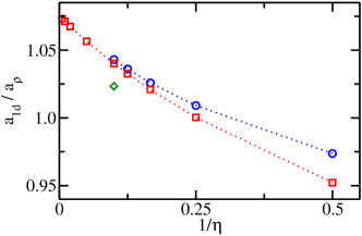
Figure 3: (Color online) Quantifying the deviations between the full three-dimensional and approximate one-dimensional treatment for the energetically lowest lying molecular branch as a function of $1/\eta$. The squares, circles and diamond show the scattering length $a_{1\text{d}}$ for which the full three-dimensional and the approximate one-dimensional zero-range interaction energies deviate by 50% for the $(1,1)$, $(2,1)$ and $(3,1)$ systems, respectively. For the $(1,1)$ and $(2,1)$ systems, dotted lines are shown as a guide to the eye.

It can be seen that the $a_{1\text{d}}/a_{\rho}$ value depends only weakly on $\eta$. Moreover, for the impurity problem considered, the $a_{1\text{d}}/a_{\rho}$ value depends only weakly on $N$. If we look for the $a_{1\text{d}}/a_{\rho}$ values for which $\epsilon$ takes values different from $1/2$, we find similar results [though the ordering of the curves for the different $(N-1,1)$ systems depends on the specific $\epsilon$ value considered]. This implies that the accuracy of the effective one-dimensional treatment can be estimated quite reliably from the results for the two-body problem for a single $\eta$. Intuitively, this can be understood from the fact that the $(N-1,1)$ system can be thought of as consisting of a single diatomic molecule and $N-2$ unpaired atoms.

Lastly, we estimate the dependence of the relative energies obtained from the three-dimensional treatment on the effective range $r_{\text{eff}}$, which is defined through the low-energy expansion of the free-space $s$-wave scattering phase shift $\delta_{0}(k)$, $k\cot(\delta_{0}(k))=-1/a_{3\text{d}}+r_{\text{eff}}k^{2}/2$ newton . Here, $k$ denotes the relative scattering wave vector. To quantify this dependence, we define the scaled energy difference $\delta$,

$$\delta=\frac{E_{N-1,1}^{3\text{d,int}}(r_{\text{eff}}=0)-E_{N-1,1}^{3\text{d,int}}(r_{\text{eff}}\neq 0)}{|E_{N-1,1}^{3\text{d,int}}(r_{\text{eff}}=0)|},$$ (15)

where the energies $E_{N-1,1}^{3\text{d,int}}(r_{\text{eff}}=0)$ and $E_{N-1,1}^{3\text{d,int}}(r_{\text{eff}}\neq 0)$ are the zero-range and finite-range interaction energies, respectively. Figures 4(a) and 4(b)

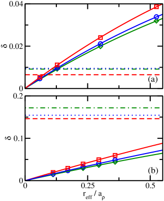
Figure 4: (Color online) Quantifying the finite-range effects of the full three-dimensional energies for $\eta=10$. (a) Squares, circles and diamonds show the scaled energy difference $\delta$ at $a_{z}/a_{3\text{d}}=-10$ as a function of the effective range $r_{\text{eff}}$ for the $(1,1)$, $(2,1)$ and $(3,1)$ systems, respectively. (b) Squares, circles and diamonds show the scaled energy difference $\delta$ at $a_{z}/a_{3\text{d}}=-2$ as a function of the effective range $r_{\text{eff}}$ for the $(1,1)$, $(2,1)$ and $(3,1)$ systems, respectively. (a) and (b): Solid lines are three-parameter fits to the numerical data. For comparison, dashed, dotted and dash-dotted lines show the scaled interaction energy difference $\epsilon$ for the $(1,1)$, $(2,1)$ and $(3,1)$ systems, respectively.

show the quantity $\delta$ for $a_{z}/a_{3\text{d}}=-10$ [$g_{1\text{d}}/(\hbar\omega_{\rho}a_{\rho})\approx-0.477$] and $a_{z}/a_{3\text{d}}=-2$ [$g_{1\text{d}}/(\hbar\omega_{\rho}a_{\rho})\approx-1.20$], respectively. Squares, circles and diamonds show the scaled energy difference for the $(1,1)$, $(2,1)$ and $(3,1)$ systems and solid lines show fits to the numerical data. To compare the finite-range effects with the difference between the three-dimensional and one-dimensional energies, dashed, dotted and dash-dotted lines show the scaled interaction energy difference $\epsilon$ for the $(1,1)$, $(2,1)$ and $(3,1)$ systems, respectively. For two ⁶Li atoms, the van der Waals length $r_{\text{vdW}}$ is $31.26a_{0}$ ChinReview ; Yan96 , where $a_{0}$ denotes the Bohr radius. Using the values of the $s$-wave scattering length and the van der Waals length Gao98 ; Flambaum99 , we find—for the parameters of the Heidelberg experiment Jochim3 ; thesisGerhard —$r_{\text{eff}}\approx 0.0141a_{\rho}$ for $a_{z}/a_{3\text{d}}=-10$ and $r_{\text{eff}}\approx 0.0138a_{\rho}$ for $a_{z}/a_{3\text{d}}=-2$. Inspection of Fig. 4 shows that the finite-range corrections to the interaction energy are roughly a factor of 10 and 100 smaller for $a_{z}/a_{3\text{d}}=-10$ and $a_{z}/a_{3\text{d}}=-2$, respectively, than the difference between the three- and one-dimensional energies. This implies that the finite-range effects can, to a good approximation, be neglected in analyzing cold atom experiments in highly elongated traps such as those conducted by the Heidelberg group.

IV Summary

This paper discussed the energies of Fermi gases with a single impurity under highly-elongated confinement. We presented energies for the $(1,1)$, $(2,1)$ and $(3,1)$ systems and assessed the accuracy of an effective one-dimensional Hamiltonian parametrized by the effective one-dimensional coupling constant $g_{1\text{d}}$. We focused on states that can be reached experimentally by first preparing an effectively non-interacting system and by then adiabatically changing the $s$-wave scattering length through application of an external magnetic field. As has been shown in the literature BlumeReview , the complete energy spectra of few-body systems are rather dense and exhibit avoided crossings (if the states belong to the same subspace of the full Hilbert space) and sharp crossings (if the states belong to different subspaces of the full Hilbert space).

We found, in agreement with what might be expected naively, that the validity regime of the effective one-dimensional treatment based on $H_{1\text{d}}$ [see Eq. (II)] is limited, for the molecular branch, to the regime where the one-dimensional even parity scattering length is larger than the harmonic oscillator length in the tight confinement direction. When the one-dimensional even parity scattering length is large compared to the harmonic oscillator length in the tight confinement direction, we found that the effective one-dimensional description can be improved if $g_{1\text{d}}$ is replaced by $g_{1\text{d}}^{\text{trap}}$, which explicitly accounts for trap corrections that arise from the fact that the aspect ratio $\eta$ is finite and not infinitely large. When the one-dimensional even parity scattering length is small compared to the harmonic oscillator length in the loose confinement direction, we found that the effective one-dimensional description can be improved if the leading-order energy dependence of $g_{1\text{d}}^{\text{trap}}$ is accounted for. The fact that the leading-order energy dependence of the effective-one-dimensional coupling constant can be derived from the waveguide Hamiltonian (i.e., the Hamiltonian with $\omega_{z}=0$) indicates that the physics in this regime is not unique to the trapped system but analogous to what has been found for waveguide geometries. Moreover, our analysis suggests that the accuracy of the effective one-dimensional treatment of small Fermi systems with an impurity can be assessed fairly accurately by looking at the $(1,1)$ system. Lastly, we found that finite-range effects (or equivalently, the energy-dependence of the three-dimensional scattering length $a_{3\text{d}}$) are negligible for the conditions of the Heidelberg experiment Jochim3 ; thesisGerhard .

Acknowledgement: Support by the ARO and valuable discussions with Yangqian Yan are gratefully acknowledged.

References

- (1) D. Blume, Rep. Prog. Phys. 75, 046401 (2012).
- (2) S. Giorgini, L. P. Pitaevskii, and S. Stringari, Rev. Mod. Phys. 80, 1215 (2008).
- (3) I. Bloch, J. Dalibard, and W. Zwerger, Rev. Mod. Phys. 80, 885 (2008).
- (4) C. Chin, R. Grimm, P. Julienne, and E. Tiesinga, Rev. Mod. Phys. 82, 1225 (2010).
- (5) F. Serwane, G. Zürn, T. Lompe, T. B. Ottenstein, A. N. Wenz, and S. Jochim, Science 332, 6027 (2011).
- (6) G. Zürn, F. Serwane, T. Lompe, A. N. Wenz, M. G. Ries, J. E. Bohn, and S. Jochim, Phys. Rev. Lett. 108, 075303 (2012).
- (7) S. Sala, G. Zürn, T. Lompe, A. N. Wenz, S. Murmann, F. Serwane, S. Jochim, and A. Saenz, Phys. Rev. Lett. 110, 203202 (2013).
- (8) G. Zürn, A. N. Wenz, S. Murmann, A. Bergschneider, T. Lompe, and S. Jochim, Phys. Rev. Lett. 111, 175302 (2013).
- (9) A. N. Wenz, G. Zürn, S. Murmann, I. Brouzos, T. Lompe, and S. Jochim, Science 342, 457 (2013).
- (10) G. Zürn, Few-fermion systems in one dimension, Ph.D. Thesis, Ruperto-Carola-University of Heidelberg, Germany (2012). see .
- (11) E. L. Bolda, E. Tiesinga, and P. S. Julienne, Phys. Rev. A 68, 032702 (2003).
- (12) Z. Idziaszek and T. Calarco, Phys. Rev. A 71, 050701(R) (2005).
- (13) Z. Idziaszek and T. Calarco, Phys. Rev. A 74, 022712 (2006).
- (14) C. Mora, A. Komnik, R. Egger, and A. O. Gogolin, Phys. Rev. Lett. 95, 080403 (2005).
- (15) C. Mora, R. Egger, and A. O. Gogolin, Phys. Rev. A 71, 052705 (2005).
- (16) G. Zürn, T. Lompe, A. N. Wenz, S. Jochim, P. S. Julienne, and J. M. Hutson, Phys. Rev. Lett. 110, 135301 (2013).
- (17) E. Fermi, Nuovo Cimento 11, 157 (1934).
- (18) K. Huang and C. N. Yang, Phys. Rev. 105, 767 (1957).
- (19) K. Huang, Statistical Mechanics, 2nd Ed. (John Wiley and Sons, Inc., New York, 1963).
- (20) M. Olshanii, Phys. Rev. Lett. 81, 938 (1998).
- (21) T. Bergeman, M. G. Moore, and M. Olshanii, Phys. Rev. Lett. 91, 163201 (2003).
- (22) B. E. Granger and D. Blume, Phys. Rev. Lett. 92, 133202 (2004).
- (23) S. E. Gharashi, K. M. Daily, and D. Blume, Phys. Rev. A 86, 042702 (2012).
- (24) D. Blume and D. Rakshit, Phys. Rev. A 80, 013601 (2009).
- (25) T. Busch, B.-G. Englert, K. Rza̧żewski, and M. Wilkens, Found. Phys. 28, 549 (1998).
- (26) S. E. Gharashi and D. Blume, Phys. Rev. Lett. 111, 045302 (2013).
- (27) J. Mitroy, S. Bubin, W. Horiuchi, Y. Suzuki, L. Adamowicz, W. Cencek, K. Szalewicz, J. Komasa, D. Blume, and K. Varga, Rev. Mod. Phys. 85, 693 (2013).
- (28) Y. Suzuki and K. Varga. Stochastic Variational Approach to Quantum Mechanical Few-Body Problems. Springer Verlag, Berlin (1998).
- (29) The parity is positive (negative) if the wavefunction does not (does) change sign under the operation that sends all to . The parity is positive (negative) if the wavefunction does not (does) change sign under the operation that sends all to and all to .
- (30) P. R. Johnson, E. Tiesinga, J. V. Porto, and C. J. Williams, New J. Phys. 11, 093022 (2009).
- (31) P. R. Johnson, D. Blume, X. Y. Yin, W. F. Flynn, and E. Tiesinga, New J. Phys. 14, 053037 (2012).
- (32) D. S. Petrov, V. Lebedev, and J. T. M. Walraven, Phys. Rev. A 85, 062711 (2012).
- (33) R. G. Newton, Scattering Theory of Waves and Particles, Second Edition, Dover Publications, Inc., Mineola and New York, 2002.
- (34) Z.-C. Yan, J. F. Babb, A. Dalgarno, and G. W. F. Drake, Phys. Rev. A 54, 2824 (1996).
- (35) B. Gao, Phys. Rev. A 58, 4222 (1998).
- (36) V. V. Flambaum, G. F. Gribakin, and C. Harabati, Phys. Rev. A 59, 1998 (1999).