Optimum design accounting for the global nonlinear behavior of the model

Abstract

Among the major difficulties that one may encounter when estimating parameters in a nonlinear regression model are the nonuniqueness of the estimator, its instability with respect to small perturbations of the observations and the presence of local optimizers of the estimation criterion.

We show that these estimability issues can be taken into account at the design stage, through the definition of suitable design criteria. Extensions of $E$-, $c$- and $G$-optimality criteria are considered, which when evaluated at a given $\theta^{0}$ (local optimal design), account for the behavior of the model response $\eta(\theta)$ for $\theta$ far from $\theta^{0}$. In particular, they ensure some protection against close-to-overlapping situations where $\|\eta(\theta)-\eta(\theta^{0})\|$ is small for some $\theta$ far from $\theta^{0}$. These extended criteria are concave and necessary and sufficient conditions for optimality (equivalence theorems) can be formulated. They are not differentiable, but when the design space is finite and the set $\Theta$ of admissible $\theta$ is discretized, optimal design forms a linear programming problem which can be solved directly or via relaxation when $\Theta$ is just compact. Several examples are presented.

and t1Supported by the VEGA Grant No. 1/0163/13.

1 Introduction

We consider a nonlinear regression model with observations

$$y_{i}=y(x_{i})=\eta(x_{i},\bar{\theta})+\varepsilon_{i},\qquad i=1,\ldots,N,$$

where the errors $\varepsilon_{i}$ satisfy $\mathbb{E}(\varepsilon_{i})=0$, $\operatorname{var}(\varepsilon_{i})=\sigma^{2}$ and $\operatorname{cov}(\varepsilon_{i},\varepsilon_{j})=0$ for $i\neq j$, $i,j=1,\ldots,N$, and the true value $\bar{\theta}$ of the vector of model parameter $\theta$ belongs to $\Theta$, a compact subset of $\mathbb{R}^{p}$ such that $\Theta\subset\overline{\operatorname{int}(\Theta)}$, the closure of the interior of $\Theta$. In a vector notation, we write

$$\mathbf{y}=\eta_{X}(\bar{\theta})+\varepsilon\qquad\mbox{with }\mathbb{E}(\varepsilon)=\mathbf{0},\operatorname{Var}(\varepsilon)=\sigma^{2}\mathbf{I}_{N},$$ (1)

where $\eta_{X}(\theta)=(\eta(x_{1},\theta),\ldots,\eta(x_{N},\theta))^{\top}$, $\mathbf{y}=(y_{1},\ldots,y_{N})^{\top}$, $\varepsilon=(\varepsilon_{1},\ldots,\varepsilon_{N})^{\top}$, and $X$ denotes the $N$-point exact design $(x_{1},\ldots,x_{N})$. The more general nonstationary (heteroscedastic) case where $\operatorname{var}(\varepsilon_{i})=\sigma^{2}(x_{i})$ can easily be transformed into the model (1) with $\sigma^{2}=1$ via the division of $y_{i}$ and $\eta(x_{i},\theta)$ by $\sigma(x_{i})$. We suppose that $\eta(x,\theta)$ is twice continuously differentiable with respect to $\theta\in\operatorname{int}(\Theta)$ for any $x\in\mathscr{X}$, a compact subset of $\mathbb{R}^{d}$. The model is assumed to be identifiable over $\mathscr{X}$; that is, we suppose that

$$\eta\bigl{(}x,\theta^{\prime}\bigr{)}=\eta(x,\theta)\qquad\mbox{for all }x\in\mathscr{X}\Longrightarrow\theta^{\prime}=\theta.$$ (2)

We shall denote by $\Xi$ the set of design measures $\xi$, that is, of probability measures on $\mathscr{X}$. The information matrix (for $\sigma^{2}=1$) for the design $X$ at $\theta$ is

$$\mathbf{M}(X,\theta)=\sum_{i=1}^{N}\frac{\partial\eta(x_{i},\theta)}{\partial\theta}\frac{\partial\eta(x_{i},\theta)}{\partial\theta^{\top}}$$

and, for any $\xi\in\Xi$, we shall write

$$\mathbf{M}(\xi,\theta)=\int_{\mathscr{X}}\bigl{[}\partial\eta(x,\theta)/\partial\theta\bigr{]}\bigl{[}\partial\eta(x,\theta)/\partial\theta^{\top}\bigr{]}\xi(\mathrm{d}x).$$

Denoting $\xi_{N}=(1/N)\sum_{i=1}^{N}\delta_{x_{i}}$ the empirical design measure associated with $X$, with $\delta_{x}$ the delta measure at $x$, we have $\mathbf{M}(X,\theta)=N\mathbf{M}(\xi_{N},\theta)$. Note that (2) implies the existence of a $\xi\in\Xi$ satisfying the Least-Squares (LS) estimability condition

$$\eta\bigl{(}x,\theta^{\prime}\bigr{)}=\eta(x,\theta)\qquad\xi\mbox{-almost everywhere}\Longrightarrow\theta^{\prime}=\theta.$$ (3)

Given an exact $N$-point design $X$, the set of all hypothetical means of the observed vectors $\mathbf{y}$ in the sample space $\mathbb{R}^{N}$ forms the expectation surface $\mathbb{S}_{\eta}=\{\eta_{X}(\theta)\dvtx\theta\in\Theta\}$. Since $\eta_{X}(\theta)$ is supposed to have continuous first- and second-order derivatives in $\operatorname{int}(\Theta)$, $\mathbb{S}_{\eta}$ is a smooth surface in $\mathbb{R}^{N}$ with a (local) dimension given by $r=\operatorname{rank}[\partial\eta_{X}(\theta)/\partial\theta^{\top}]$. If $r=p$ (which means full rank), the model (1) is said regular. In regular models with no overlapping of $\mathbb{S}_{\eta}$, that is, when $\eta_{X}(\theta)=\eta_{X}(\theta^{\prime})$ implies $\theta=\theta^{\prime}$, the LS estimator

$$\hat{\theta}_{\mathrm{LS}}=\hat{\theta}_{\mathrm{LS}}^{N}=\arg\min_{\theta\in\Theta}\bigl{\|}\mathbf{y}-\eta_{X}(\theta)\bigr{\|}^{2}$$ (4)

is uniquely defined with probability one (w.p.1). Indeed, when the distributions of errors $\varepsilon_{i}$ have probability densities (in the standard sense) it can be proven that $\eta[\hat{\theta}_{\mathrm{LS}}(\mathbf{y})]$ is unique w.p.1; see Pázman (1984) and Pázman (1993), page 107. However, there is still a positive probability that the function $\theta\longrightarrow\|\mathbf{y}-\eta_{X}(\theta)\|^{2}$ has a local minimizer different from the global one when the regression model is intrinsically curved in the sense of Bates and Watts (1980), that is, when $\mathbb{S}_{\eta}$ is a curved surface in $\mathbb{R}^{N}$; see Demidenko (1989, 2000). Moreover, a curved surface can “almost overlap”; that is, there may exist points $\theta$ and $\theta^{\prime}$ in $\Theta$ such that $\|\theta^{\prime}-\theta\|$ is large but $\|\eta_{X}(\theta^{\prime})-\eta_{X}(\theta)\|$ is small (or even equals zero in case of strict overlapping). This phenomenon can cause serious difficulties in parameter estimation, leading to instabilities of the estimator, and one should thus attempt to reduce its effects by choosing an adequate experimental design. Classically, those issues are ignored at the design stage and the experiment is chosen on the basis of asymptotic local properties of the estimator. Even when the design relies on small-sample properties of the estimator, like in Pázman and Pronzato (1992), Gauchi and Pázman (2006), a nonoverlapping assumption is used [see Pázman (1993), pages 66 and 157] which permits to avoid the aforementioned difficulties. Note that putting restrictions on curvature measures is not enough: consider the case $\operatorname{dim}(\theta)=1$ with the overlapping $\mathbb{S}_{\eta}$ formed by a circle of arbitrarily large radius, and thus arbitrarily small curvature (see the example in Section 2 below).

Important and precise results are available concerning the construction of subsets of $\Theta$ where such difficulties are guaranteed not to occur; see, for example, Chavent (1983, 1990, 1991); however, their exploitation for choosing adequate designs is far from straightforward. Also, the construction of designs with restricted curvatures, as proposed by Clyde and Chaloner (2002), is based on the curvature measures of Bates and Watts (1980) and uses derivatives of $\eta_{X}(\theta)$ at a certain $\theta$; this local approach is unable to catch the problem of overlapping for two points that are distant in the parameter space. Other design criteria using a second-order development of the model response, or an approximation of the density of $\hat{\theta}_{\mathrm{LS}}$ [Hamilton and Watts (1985), Pronzato and Pázman (1994)], are also inadequate.

The aim of this paper is to present new optimality criteria for optimum design in nonlinear regression models that may reduce such effects, especially overlapping, and are at the same time closely related to classical optimality criteria like $E$-, $c$- or $G$-optimality (in fact, they coincide with those criteria when the regression model is linear). Classical optimality criteria focus on efficiency, that is, aim at ensuring a precise estimation of $\theta$, asymptotically, provided that the model is locally identifiable at $\theta$. On the other hand, the new extended criteria account for the global behavior of the model and enforce identifiability.

An elementary example is given in the next section and illustrates the motivation of our work. The criterion of extended $E$-optimality is considered in Section 3; its main properties are detailed and algorithms for the construction of optimal designs are presented. Sections 4 and 5 are, respectively, devoted to the criteria of extended $c$-optimality and extended $G$-optimality. Several illustrative examples are presented in Section 6. Section 7 suggests some extensions and further developments and Section 8 concludes.

2 An elementary motivating example

Example 1.

Suppose that $\theta\in\Theta=[0,1]$ and that, for any design point $x=(t,u)^{\top}\in\mathscr{X}=\{0,\pi/2\}\times[0,u_{\max}]$, we have

$$\eta(x,\theta)=r\cos(t-u\theta),$$

with $r$ a known positive constant. We take $u_{\max}=7\pi/4$; the difficulties mentioned below are even more pronounced for values of $u_{\max}$ closer to $2\pi$. We shall consider exclusively two-point designs $X=(x_{1},x_{2})$ of the form

$$x_{1}=(0,u)^{\top},\qquad x_{2}=(\pi/2,u)^{\top}$$

and denote $\nu_{u}$ the associated design measure, $\nu_{u}=(1/2)[\delta_{x_{1}}+\delta_{x_{2}}]$. We shall look for an optimal design, that is, an optimal choice of $u\in[0,u_{\max}]$, where optimality is considered in terms of information.

It is easy to see that for any design $\nu_{u}$ we have

$$\eta_{X}(\theta)=\pmatrix{\eta(x_{1},\theta)\cr\eta(x_{2},\theta)}=\pmatrix{r\cos(u\theta)\cr r\sin(u\theta)}.$$

The expectation surface is then an arc of a circle, with central angle $u$; see Figure 1 for the case $u=u_{\max}=7\pi/4$. The model is nonlinear but parametrically linear since the information matrix $M(X,\theta)$ for $\sigma^{2}=1$ (here scalar since $\theta$ is scalar) equals $r^{2}u^{2}$ and does not depend on $\theta$. Also, the intrinsic curvature (see Section 6) is constant and equals $1/r$, and the model is also almost intrinsically linear if $r$ gets large.

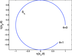
Figure 1: Expectation surface $\mathbb{S}_{\eta}$ for $\theta\in\Theta=[0,1]$, $r=1$ and $u=u_{\max}=7\pi/4$.

Any classical optimality criterion ($A$-, $D$-, $E$-) indicates that one should observe at $u=u_{\max}$, and setting a constraint on the intrinsic curvature is not possible here. However, if the true value of $\theta$ is $\bar{\theta}=0$ and $\sigma^{2}$ is large enough, there is a chance that the LS estimator will be $\hat{\theta}_{\mathrm{LS}}=1$, and thus very far from $\bar{\theta}$; see Figure 1. The situation gets even worse if $u_{\max}$ gets closer to $2\pi$, since $\mathbb{S}_{\eta}$ then almost overlaps.

Now, consider $H_{E}(\nu_{u},\theta)=(1/2)\|\eta_{X}(\theta)-\eta_{X}(\theta^{0})\|^{2}/|\theta-\theta^{0}|^{2}$, see (5), with $\theta^{0}=0$. For all $u\in[0,u_{\max}]$, the minimum of $H_{E}(\nu_{u},\theta)$ with respect to $\theta\in\Theta$ is obtained at $\theta=1$, $H_{E}(\nu_{u},1)=r^{2}[1-\cos(u)]$ is then maximum in $[0,u_{\max}]$ for $u=u_{*}=\pi$. This choice $u=u_{*}$ seems preferable to $u=u_{\max}$ since the expectation surface $\mathbb{S}_{\eta}$ is then a half-circle, so that $\eta_{X}(0)$ and $\eta_{X}(1)$ are as far away as possible. On the other hand, as shown in Section 3, $\min_{\theta\in\Theta}H_{E}(\nu_{u},\theta)$ possesses most of the attractive properties of classical optimality criteria and even coincides with one of them in linear models.

Figure 2-left shows $H_{E}(\nu_{u},\theta)$ as a function of $\theta$ for three values of $u$ and illustrates the fact that the minimum of $H_{E}(\nu_{u},\theta)$ with respect to $\theta\in\Theta$ is maximized for $u=u_{*}$. Figure 2-right shows that the design with $u=u_{\max}$ (dashed line) is optimal locally at $\theta=\theta^{0}$, in the sense that it yields the fastest increase of $\|\eta_{X}(\theta)-\eta_{X}(\theta^{0})\|$ as $\theta$ slightly deviates from $\theta^{0}$. On the other hand, $u=\pi$ maximizes $\min_{\theta\in\Theta}\|\eta_{X}(\theta)-\eta_{X}(\theta^{0})\|/|\theta-\theta^{0}|$ (solid line) and realizes a better protection against the folding effect of $\mathbb{S}_{\eta}$, at the price of a slightly less informative experiment for $\theta$ close to $\theta^{0}$. Smaller values of $u$ (dotted line) are worse than $u_{*}$, both locally for $\theta$ close to $\theta^{0}$ and globally in terms of the folding of $\mathbb{S}_{\eta}$.

The rest of the paper will formalize these ideas and show how to implement them for general nonlinear models through the definition of suitable design criteria that can be easily optimized.

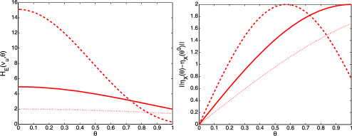
Figure 2: $H_{E}(\nu_{u},\theta)$ (left) and $\|\eta_{X}(\theta)-\eta_{X}(\theta^{0})\|$ (right) as functions of $\theta\in\Theta=[0,1]$ for $r=1$, $u=2$ (dotted line), $u=u_{\max}=7\pi/4$ (dashed line) and $u=u_{*}=\pi$ (solid line).

3 Extended (globalized) $E$-optimality

3.1 Definition of $\phi_{eE}(\cdot)$

Take a fixed point $\theta^{0}$ in $\Theta$ and denote

$$H_{E}(\xi,\theta)=H_{E}\bigl{(}\xi,\theta;\theta^{0}\bigr{)}=\frac{\|\eta(\cdot,\theta)-\eta(\cdot,\theta^{0})\|_{\xi}^{2}}{\|\theta-\theta^{0}\|^{2}},$$ (5)

where $\|\cdot\|_{\xi}$ denotes the norm in $\mathscr{L}_{2}(\xi)$; that is, $\|l\|_{\xi}=[\int_{\mathscr{X}}l^{2}(x)\xi(\mathrm{d}x)]^{1/2}$ for any $l\in\mathscr{L}_{2}(\xi)$. When $\xi$ is a discrete measure, like in the examples considered in the paper, then $\|l\|_{\xi}^{2}$ is simply the sum $\sum_{x:\xi(\{x\})>0}\xi(\{x\})l^{2}(x)$.

The extended $E$-optimality criterion is defined by

$$\phi_{eE}(\xi)=\phi_{eE}\bigl{(}\xi;\theta^{0}\bigr{)}=\min_{\theta\in\Theta}H_{E}(\xi,\theta),$$ (6)

to be maximized with respect to the design measure $\xi$.

In a nonlinear regression model $\phi_{eE}(\cdot)$ depends on the value chosen for $\theta^{0}$ and can thus be considered as a local optimality criterion. On the other hand, the criterion is global in the sense that it depends on the behavior of $\eta(\cdot,\theta)$ for $\theta$ far from $\theta^{0}$. This (limited) locality can be removed by considering $\phi_{MeE}(\xi)=\min_{\theta^{0}\in\Theta}\phi_{eE}(\xi;\theta^{0})$ instead of (6), but only the case of $\phi_{eE}(\cdot)$ will be detailed in the paper, the developments being similar for $\phi_{MeE}(\cdot)$; see Section 7.2.

For a linear regression model with $\eta(x,\theta)=\mathbf{f}^{\top}(x)\theta+v(x)$ and $\Theta=\mathbb{R}^{p}$, for any $\theta^{0}$ and any $\xi\in\Xi$, we have $\|\eta(\cdot,\theta)-\eta(\cdot,\theta^{0})\|_{\xi}^{2}=(\theta-\theta^{0})^{\top}\mathbf{M}(\xi)(\theta-\theta^{0})$, so that

$$\phi_{eE}(\xi)=\min_{\theta-\theta^{0}\in\mathbb{R}^{p}}\frac{(\theta-\theta^{0})^{\top}\mathbf{M}(\xi)(\theta-\theta^{0})}{\|\theta-\theta^{0}\|^{2}}=\lambda_{\min}\bigl{[}\mathbf{M}(\xi)\bigr{]},$$

the minimum eigenvalue of $\mathbf{M}(\xi)$, and corresponds to the $E$-optimality criterion.

For a nonlinear model with $\Theta=\mathscr{B}(\theta^{0},\rho)$, the ball with center $\theta^{0}$ and radius $\rho$, direct calculation shows that

$$\lim_{\rho\rightarrow 0}\phi_{eE}\bigl{(}\xi;\theta^{0}\bigr{)}=\lambda_{\min}\bigl{[}\mathbf{M}\bigl{(}\xi,\theta^{0}\bigr{)}\bigr{]}.$$ (7)

In a nonlinear regression model with larger $\Theta$, the determination of an optimum design $\xi_{eE}^{*}$ maximizing $\phi_{eE}(\xi)$ ensures some protection against $\|\eta(\cdot,\theta)-\eta(\cdot,\theta^{0})\|_{\xi}$ being small for some $\theta$ far from $\theta^{0}$. In particular, when $\theta^{0}\in\operatorname{int}(\Theta)$ then $\phi_{eE}(\xi;\theta^{0})=0$ if either $\mathbf{M}(\xi,\theta^{0})$ is singular or $\|\eta(\cdot,\theta)-\eta(\cdot,\theta^{0})\|_{\xi}=0$ for some $\theta\neq\theta^{0}$. Therefore, under the condition (2), $\xi_{eE}^{*}$ satisfies the estimability condition (3) at $\theta=\theta^{0}$ and is necessarily nondegenerate, that is, $\mathbf{M}(\xi_{eE}^{*},\theta^{0})$ is nonsingular, when $\theta^{0}\in\operatorname{int}(\Theta)$ (provided that there exists a nondegenerate design in $\Xi$). Notice that (7) implies that $\phi_{eE}(\xi;\theta^{0})\leq\lambda_{\min}[\mathbf{M}(\xi,\theta^{0})]$ when $\Theta$ contains some open neighborhood of $\theta^{0}$. In contrast with the $E$-optimality criterion, maximizing $\phi_{eE}(\xi;\theta^{0})$ in nonlinear models does not require computation of the derivatives of $\eta(x,\theta)$ with respect to $\theta$ at $\theta^{0}$; see the algorithms proposed in Sections 3.3 and 3.4. Also note that the influence of points that are very far from $\theta^{0}$ can be suppressed by modification of the denominator of (5) without changing the relation with $E$-optimality; see Section 7.1.

Before investigating properties of $\phi_{eE}(\cdot)$ as a criterion function for optimum design in the next section, we state a property relating $\phi_{eE}(\xi)$ to the localization of the LS estimator $\hat{\theta}_{\mathrm{LS}}$.

Theorem 1.

For any given $\theta\in\Theta$, the LS estimator $\hat{\theta}_{\mathrm{LS}}$ given by (4) in the model (1) satisfies

$$\hat{\theta}_{\mathrm{LS}}\in\Theta\cap\mathscr{B}\biggl{(}\theta,\frac{2\|\mathbf{y}-\eta_{X}(\theta)\|}{\sqrt{N}\sqrt{\phi_{eE}(\xi_{N};\theta)}}\biggr{)},$$

with $\xi_{N}$ the empirical measure associated with the design $X$ used to observe $\mathbf{y}$.

The result follows from the following chain of inequalities:

$$\|\hat{\theta}_{\mathrm{LS}}-\theta\| \leq \frac{\|\eta(\cdot,\hat{\theta}_{\mathrm{LS}})-\eta(\cdot,\theta)\|_{\xi_{N}}}{\sqrt{\phi_{eE}(\xi_{N};\theta)}}=\frac{\|\eta_{X}(\hat{\theta}_{\mathrm{LS}})-\eta_{X}(\theta)\|}{\sqrt{N}\sqrt{\phi_{eE}(\xi_{N};\theta)}}$$ (8)

$$\leq \frac{\|\mathbf{y}-\eta_{X}(\hat{\theta}_{\mathrm{LS}})\|+\|\mathbf{y}-\eta_{X}(\theta)\|}{\sqrt{N}\sqrt{\phi_{eE}(\xi_{N};\theta)}}\leq\frac{2\|\mathbf{y}-\eta_{X}(\theta)\|}{\sqrt{N}\sqrt{\phi_{eE}(\xi_{N};\theta)}}.$$

Note that although the bound (8) is tight in general nonlinear situations (due to the possibility that $\mathbb{S}_{\eta}$ overlaps), it is often pessimistic. In particular, in the linear regression model $\eta(x,\theta)=\mathbf{f}^{\top}(x)\theta+v(x)$, direct calculation gives

$$\|\hat{\theta}_{\mathrm{LS}}-\theta\|\leq\sqrt{\lambda_{\max}\bigl{[}\bigl{(}\mathbf{F}^{\top}\mathbf{F}\bigr{)}^{-1}\bigr{]}}\bigl{\|}\mathbf{y}-\eta_{X}(\theta)\bigr{\|}=\frac{\|\mathbf{y}-\eta_{X}(\theta)\|}{\sqrt{N}\sqrt{\phi_{eE}(\xi_{N})}},$$

where $\mathbf{F}$ is the $N\times p$ matrix with $i$th line equal to $\mathbf{f}^{\top}(x_{i})$. We also have $\|\hat{\theta}_{\mathrm{LS}}-\theta\|\leq\|\mathbf{y}-\eta_{X}(\theta)\|/[\sqrt{N}\sqrt{\phi_{eE}(\xi_{N},\theta)}]$ in intrinsically linear models (with a flat expectation surface $\mathbb{S}_{\eta}$) since then $\|\eta_{X}(\hat{\theta}_{\mathrm{LS}})-\eta_{X}(\theta)\|\leq\|\mathbf{y}-\eta_{X}(\theta)\|$.

In the following, we shall omit the dependence in $\theta^{0}$ and simply write $\phi_{eE}(\xi)$ for $\phi_{eE}(\xi;\theta^{0})$ when there is no ambiguity.

3.2 Properties of $\phi_{eE}(\cdot)$

As the minimum of linear functions of $\xi$, $\phi_{eE}(\cdot)$ is concave: for all $\xi,\nu\in\Xi$ and all $\alpha\in[0,1]$, $\phi_{eE}[(1-\alpha)\xi+\alpha\nu]\geq(1-\alpha)\phi_{eE}(\xi)+\alpha\phi_{eE}(\nu)$. It is also positively homogeneous: $\phi_{eE}(a\xi)=a\phi_{eE}(\xi)$ for all $\xi\in\Xi$ and $a>0$; see, for example, Pukelsheim (1993), Chapter 5. The criterion of ${eE}$-efficiency can then be defined as

$$\mathscr{E}_{eE}(\xi)=\frac{\phi_{eE}(\xi)}{\phi_{eE}(\xi_{eE}^{*})},\qquad\xi\in\Xi,$$

where $\xi_{eE}^{*}$ maximizes $\phi_{eE}(\xi)$.

The concavity of $\phi_{eE}(\cdot)$ implies the existence of directional derivatives and, due to the linearity in $\xi$ of $H_{E}(\xi,\theta)$, we have the following; see, for example, Dem’yanov and Malozemov (1974).

Theorem 2.

For any $\xi,\nu\in\Xi$, the directional derivative of the criterion $\phi_{eE}(\cdot)$ at $\xi$ in the direction $\nu$ is given by

$$F_{\phi_{eE}}(\xi;\nu)=\min_{\theta\in\Theta_{E}(\xi)}H_{E}(\nu,\theta)-\phi_{eE}(\xi),$$

where $\Theta_{E}(\xi)=\{\theta\in\Theta\dvtx H_{E}(\xi,\theta)=\phi_{eE}(\xi)\}$.

Note that we can write $F_{\phi_{eE}}(\xi;\nu)=\min_{\theta\in\Theta_{E}(\xi)}\int_{\mathscr{X}}\Psi_{eE}(x,\theta,\xi)\nu(\mathrm{d}x)$, where

$$\Psi_{eE}(x,\theta,\xi)=\frac{[\eta(x,\theta)-\eta(x,\theta^{0})]^{2}-\|\eta(\cdot,\theta)-\eta(\cdot,\theta^{0})\|_{\xi}^{2}}{\|\theta-\theta^{0}\|^{2}}.$$ (9)

Due to the concavity of $\phi_{eE}(\cdot)$, a necessary and sufficient condition for the optimality of a design measure $\xi_{eE}^{*}$ is that

$$\sup_{\nu\in\Xi}F_{\phi_{eE}}\bigl{(}\xi_{eE}^{*};\nu\bigr{)}=0,$$ (10)

a condition often called “equivalence theorem” in optimal design theory; see, for example, Fedorov (1972), Silvey (1980). An equivalent condition is as follows.

Theorem 3.

A design $\xi_{eE}^{*}\in\Xi$ is optimal for $\phi_{eE}(\cdot)$ if and only if

$$\max_{x\in\mathscr{X}}\int_{\Theta_{E}(\xi_{eE}^{*})}\Psi_{eE}(x,\theta,\xi)\mu^{*}(\mathrm{d}\theta)=0$$

(11)

$$\eqntext{\mbox{for some measure $\mu^{*}\in\mathscr{M}\bigl{[}\Theta_{E}\bigl{(}\xi_{eE}^{*}\bigr{)}\bigr{]}$},}$$ (12)

the set of probability measures on $\Theta_{E}(\xi_{eE}^{*})$.

This is a classical result for maximin design problems; see, for example, Fedorov and Hackl (1997), Section 2.6. We have

$$0 \leq \sup_{\nu\in\Xi}F_{\phi_{eE}}(\xi;\nu)$$ (13)

$$= \sup_{\nu\in\Xi}\min_{\theta\in\Theta_{E}(\xi)}\int_{\mathscr{X}}\Psi_{eE}(x,\theta,\xi)\nu(\mathrm{d}x)$$

$$= \sup_{\nu\in\Xi}\min_{\mu\in\mathscr{M}[\Theta_{E}(\xi)]}\int_{\mathscr{X}}\int_{\Theta_{E}(\xi)}\Psi_{eE}(x,\theta,\xi)\mu(\mathrm{d}\theta)\nu(\mathrm{d}x)$$

$$= \min_{\mu\in\mathscr{M}[\Theta_{E}(\xi)]}\sup_{\nu\in\Xi}\int_{\mathscr{X}}\int_{\Theta_{E}(\xi)}\Psi_{eE}(x,\theta,\xi)\mu(\mathrm{d}\theta)\nu(\mathrm{d}x)$$

$$= \min_{\mu\in\mathscr{M}[\Theta_{E}(\xi)]}\max_{x\in\mathscr{X}}\int_{\Theta_{E}(\xi)}\Psi_{eE}(x,\theta,\xi)\mu(\mathrm{d}\theta).$$

Therefore, the necessary and sufficient condition (10) can be written as (3).

One should notice that $\sup_{\nu\in\Xi}F_{\phi_{eE}}(\xi;\nu)$ is generally not obtained for $\nu$ equal to a one-point (delta) measure, which prohibits the usage of classical vertex-direction algorithms for optimizing $\phi_{eE}(\cdot)$. Indeed, the minimax problem (13) has generally several solutions $x^{(i)}$ for $x$, $i=1,\ldots,s$, and the optimal $\nu^{*}$ is then a linear combination $\sum_{i=1}^{s}w_{i}\delta_{x^{(i)}}$, with $w_{i}\geq 0$ and $\sum_{i=1}^{s}w_{i}=1$; see Pronzato, Huang and Walter (1991) for developments on a similar difficulty in $T$-optimum design for model discrimination. This property, due to the fact that $\phi_{eE}(\cdot)$ is not differentiable, has the important consequence that the determination of a maximin-optimal design cannot be obtained via standard design algorithms used for differentiable criteria.

To avoid that difficulty, a regularized version $\phi_{eE,\lambda}(\cdot)$ of $\phi_{eE}(\cdot)$ is considered in Pronzato and Pázman (2013), Sections 7.7.3 and 8.3.2, with the property that $\lim_{\lambda\rightarrow\infty}\phi_{eE,\lambda}(\xi)=\phi_{eE}(\xi)$ for any $\xi\in\Xi$ (the convergence being uniform when $\Theta$ is a finite set), $\phi_{eE}(\cdot)$ is concave and such that $\sup_{\nu\in\Xi}F_{\phi_{eE,\lambda}}(\xi;\nu)$ is obtained when $\nu$ is the delta measure $\delta_{x^{*}}$ at some $x^{*}\in\mathscr{X}$ (depending on $\xi$). However, although $\phi_{eE,\lambda}(\cdot)$ is smooth for any finite $\lambda$, its maximization tends to be badly conditioned for large $\lambda$.

In the next section, we show that optimal design for $\phi_{eE}(\cdot)$ reduces to linear programming when $\Theta$ and $\mathscr{X}$ are finite. This is an important property. An algorithm based on a relaxation of the maximin problem is then considered in Section 3.4 for the case where $\Theta$ is compact.

3.3 Optimal design via linear-programming ($\Theta$ is finite)

To simplify the construction of an optimal design, one may take $\Theta$ as a finite set, $\Theta=\Theta^{(m)}=\{\theta^{(1)},\theta^{(2)},\ldots,\theta^{(m)}\}$; $\phi_{eE}(\xi)$ can then be written as $\phi_{eE}(\xi)=\min_{j=1,\ldots,m}H_{E}(\xi,\theta^{(j)})$, with $H_{E}(\xi,\theta)$ given by (5). If the design space $\mathscr{X}$ is also finite, with $\mathscr{X}=\{x^{(1)},x^{(2)},\ldots,x^{(\ell)}\}$, then the determination of an optimal design measure for $\phi_{eE}(\cdot)$ amounts to the determination of a scalar $t$ and of a vector of weights $\mathbf{w}=(w_{1},w_{2},\ldots,w_{\ell})^{\top}$, $w_{i}$ being allocated at $x^{(i)}$ for each $i=1,\ldots,\ell$, such that $\mathbf{c}^{\top}[\mathbf{w}^{\top},t]^{\top}$ is maximized, with $\mathbf{c}=(0,0,\ldots,0,1)^{\top}$ and $\mathbf{w}$ and $t$ satisfying the constraints

$$\sum_{i=1}^{\ell}w_{i} = 1,\qquad w_{i}\geq 0,i=1,\ldots,\ell,$$

$$\sum_{i=1}^{\ell}w_{i}h_{i}\bigl{(}\theta^{(j)}\bigr{)} \geq t,\qquad j=1,\ldots,m,$$

where we denoted

$$h_{i}(\theta)=\frac{[\eta(x^{(i)},\theta)-\eta(x^{(i)},\theta^{0})]^{2}}{\|\theta-\theta^{0}\|^{2}}.$$ (15)

This is a linear programming (LP) problem, which can easily be solved using standard methods (for instance, the simplex algorithm), even for large $m$ and $\ell$. We shall denote by $(\hat{\mathbf{w}},\hat{t})=\mathrm{LP}_{eE}(\mathscr{X},\Theta^{(m)})$ the solution of this problem.

We show below how a compact subset $\Theta$ of $\mathbb{R}^{p}$ with nonempty interior can be replaced by a suitable discretized version $\Theta^{(m)}$ that can be enlarged iteratively.

3.4 Optimal design via relaxation and the cutting-plane method ($\Theta$ is a compact subset of $\mathbb{R}^{p}$)

Suppose now that $\mathscr{X}$ is finite and that $\Theta$ is a compact subset of $\mathbb{R}^{p}$ with nonempty interior. In the LP formulation above, $(\mathbf{w},t)$ must satisfy an infinite number of constraints: $\sum_{i=1}^{\ell}w_{i}h_{i}(\theta)\geq t$ for all $\theta\in\Theta$; see (3.3). One may then use the method of Shimizu and Aiyoshi (1980) and consider the solution of a series of relaxed LP problems, using at step $k$ a finite set of constraints only, that is, consider $\theta\in\Theta^{(k)}$ finite. Once a solution $(\mathbf{w}^{k},t^{k})=\mathrm{LP}_{eE}(\mathscr{X},\Theta^{(k)})$ of this problem is obtained, using a standard LP solver, the set $\Theta^{(k)}$ is enlarged to $\Theta^{(k+1)}=\Theta^{(k)}\cup\{\theta^{(k+1)}\}$ with $\theta^{(k+1)}$ given by the constraint (3.3) most violated by $\mathbf{w}^{k}$, that is,

$$\theta^{(k+1)}=\arg\min_{\theta\in\Theta}H_{E}\bigl{(}\mathbf{w}^{k},\theta\bigr{)},$$ (16)

where with a slight abuse of notation, we write $H_{E}(\mathbf{w},\theta)=H_{E}(\xi,\theta)$; see (5), when $\xi$ allocates mass $w_{i}$ at the support point $x^{(i)}\in\mathscr{X}$ for all $i$. This yields the following algorithm for the maximization of $\phi_{eE}(\cdot)$.

[(1)]

Take any vector $\mathbf{w}^{0}$ of nonnegative weights summing to one, choose $\epsilon>0$, set $\Theta^{(0)}=\varnothing$ and $k=0$.

Compute $\theta^{(k+1)}$ given by (16), set $\Theta^{(k+1)}=\Theta^{(k)}\cup\{\theta^{(k+1)}\}$.

Use a LP solver to determine $(\mathbf{w}^{k+1},t^{k+1})=\mathrm{LP}_{eE}(\mathscr{X},\Theta^{(k+1)})$.

If $\Delta_{k+1}=t^{k+1}-\phi_{eE}(\mathbf{w}^{k+1})<\epsilon$, take $\mathbf{w}^{k+1}$ as an $\epsilon$-optimal solution and stop; otherwise $k\leftarrow k+1$, return to step 1.

The optimal value $\phi_{eE}^{*}=\max_{\xi\in\Xi}\phi_{eE}(\xi)$ satisfies

$$\phi_{eE}\bigl{(}\mathbf{w}^{k+1}\bigr{)}\leq\phi_{eE}^{*}\leq t^{k+1}$$

at every iteration, so that $\Delta_{k+1}$ of step 3 gives an upper bound on the distance to the optimum in terms of criterion value.

The algorithm can be interpreted in terms of the cutting-plane method. Indeed, from (5) and (15) we have $H_{E}(\mathbf{w},\theta^{(j+1)})=\sum_{i=1}^{\ell}w_{i}h_{i}(\theta^{(j+1)})$ for any vector of weights $\mathbf{w}$. From the definition of $\theta^{(j+1)}$ in (16), we obtain

$$\phi_{eE}(\mathbf{w})\leq H_{E}\bigl{(}\mathbf{w},\theta^{(j+1)}\bigr{)} = H_{E}\bigl{(}\mathbf{w}^{j},\theta^{(j+1)}\bigr{)}+\sum_{i=1}^{\ell}h_{i}\bigl{(}\theta^{(j+1)}\bigr{)}\bigl{\{}\mathbf{w}-\mathbf{w}^{j}\bigr{\}}_{i}$$

$$= \phi_{eE}\bigl{(}\mathbf{w}^{j}\bigr{)}+\sum_{i=1}^{\ell}h_{i}\bigl{(}\theta^{(j+1)}\bigr{)}\bigl{\{}\mathbf{w}-\mathbf{w}^{j}\bigr{\}}_{i},$$

so that the vector with components $h_{i}(\theta^{(j+1)})$, $i=1,\ldots,\ell$, forms a subgradient of $\phi_{eE}(\cdot)$ at $\mathbf{w}^{j}$, which we denote $\nabla\phi_{eE}(\mathbf{w}^{j})$ below [it is sometimes called supergradient since $\phi_{eE}(\cdot)$ is concave]. Each of the constraints

$$\sum_{i=1}^{\ell}w_{i}h_{i}\bigl{(}\theta^{(j+1)}\bigr{)}\geq t,$$

used in the LP problem of step 2, with $j=0,\ldots,k$, can be written as

$$\nabla^{\top}\phi_{eE}\bigl{(}\mathbf{w}^{j}\bigr{)}\mathbf{w}=\phi_{eE}\bigl{(}\mathbf{w}^{j}\bigr{)}+\nabla^{\top}\phi_{eE}\bigl{(}\mathbf{w}^{j}\bigr{)}\bigl{(}\mathbf{w}-\mathbf{w}^{j}\bigr{)}\geq t.$$

Therefore, $\mathbf{w}^{k+1}$ determined at step 2 maximizes the piecewise-linear approximation

$$\min_{j=0,\ldots,k}\bigl{\{}\phi_{eE}\bigl{(}\mathbf{w}^{j}\bigr{)}+\nabla^{\top}\phi_{eE}\bigl{(}\mathbf{w}^{j}\bigr{)}\bigl{(}\mathbf{w}-\mathbf{w}^{j}\bigr{)}\bigr{\}}$$

of $\phi_{eE}(\mathbf{w})$ with respect to the vector of weights $\mathbf{w}$, and the algorithm corresponds to the cutting-plane method of Kelley (1960).

The only difficult step in the algorithm corresponds to the determination of $\theta^{(k+1)}$ in (16) when $\Theta$ is a compact set. We found that the following simple procedure is rather efficient. Construct a finite grid, or a space-filling design, $\mathscr{G}^{0}$ in $\Theta$. Then, for $k=0,1,2,\ldots$

$$\cases{\phantom{ii}\mathrm{(i)}&\quad$\mbox{compute }\hat{\theta}^{k+1}=\displaystyle\arg\min_{\theta^{\prime}\in\mathscr{G}^{k}}H_{E}\bigl{(}\mathbf{w}^{k},\theta^{\prime}\bigr{)};$\vspace*{2pt}\cr\phantom{i}\mathrm{(ii)}&\quad$\mbox{perform a local minimization of }H_{E}\bigl{(}\mathbf{w}^{k},\theta\bigr{)}$\vspace*{2pt}\cr&\quad$\mbox{with respect to }\theta\in\Theta,\mbox{ initialized at }\hat{\theta}^{k+1};$\vspace*{2pt}\cr&\quad$\mbox{let }\theta^{(k+1)}\mbox{ denote the solution};$\vspace*{2pt}\cr\mathrm{(iii)}&\quad$\mbox{set }\mathscr{G}^{k+1}=\mathscr{G}^{k}\cup\bigl{\{}\theta^{(k+1)}\bigr{\}}.$}$$ (17)

The optimal value $\phi_{eE}(\xi^{*}_{eE})$ can then be approximated by $H_{E}(\mathbf{w}^{k+1},\theta^{(k+2)})$ when the algorithm stops (step 3).

The method of cutting planes is known to have sometimes rather poor convergence properties; see, for example, Bonnans et al. (2006), Chapter 9, Nesterov (2004), Section 3.3.2. A significant improvement consists in restricting the search for $\mathbf{w}^{k+1}$ at step 2 to some neighborhood of the best solution obtained so far, which forms the central idea of bundle methods; see Lemaréchal, Nemirovskii and Nesterov (1995), Bonnans et al. (2006), Chapters 9–10. In particular, the level method of Nesterov (2004), Section 3.3.3, adds a quadratic-programming step to each iteration of the cutting planes algorithm presented above; one may refer for instance to Pronzato and Pázman (2013), Section 9.5.3, for an application of the level method to design problems. Notice that any linear constraint on $\mathbf{w}$ can easily be taken into account in addition to those in (3.3), so that the method directly applies to optimal design with linear cost-constraints; see, for example, Fedorov and Leonov (2014), Section 4.2.

4 Extended (globalized) $c$-optimality

4.1 Definition and properties

Consider the case where one wants to estimate a scalar function of $\theta$, denoted by $g(\theta)$, possibly nonlinear. We assume that

$$\mathbf{c}=\mathbf{c}(\theta)=\frac{\partial g(\theta)}{\partial\theta}\bigg{|}_{\theta=\theta^{0}}\neq\mathbf{0}.$$

Denote

$$H_{c}(\xi,\theta)=H_{c}\bigl{(}\xi,\theta;\theta^{0}\bigr{)}=\frac{\|\eta(\cdot,\theta)-\eta(\cdot,\theta^{0})\|_{\xi}^{2}}{|g(\theta)-g(\theta^{0})|^{2}}$$ (18)

and consider the design criterion defined by

$$\phi_{ec}(\xi)=\min_{\theta\in\Theta}H_{c}(\xi,\theta),$$ (19)

to be maximized with respect to the design measure $\xi$.

When $\eta(x,\theta)$ and the scalar function $g(\theta)$ are both linear in $\theta$, with $g(\theta)=\mathbf{c}^{\top}\theta$, we get

$$\phi_{ec}(\xi)=\min_{\theta\in\Theta,\mathbf{c}^{\top}(\theta-\theta^{0})\neq 0}\frac{(\theta-\theta^{0})^{\top}\mathbf{M}(\xi)(\theta-\theta^{0})}{[\mathbf{c}^{\top}(\theta-\theta^{0})]^{2}}$$

and, therefore, $\phi_{ec}(\xi)=[\mathbf{c}^{\top}\mathbf{M}^{-}(\xi)\mathbf{c}]^{-1}$, using the well-known formula$\mathbf{c}^{\top}\mathbf{M}^{-}\mathbf{c}=\max_{\alpha\neq 0}(\mathbf{c}^{\top}\alpha)^{2}/(\alpha^{\top}\mathbf{M}\alpha)$; cf. Harville (1997), equation (10.4). Also, for a nonlinear model with $\Theta=\mathscr{B}(\theta^{0},\rho)$ and a design $\xi$ such that $\mathbf{M}(\xi,\theta^{0})$ has full rank, one has

$$\lim_{\rho\rightarrow 0}\phi_{ec}(\xi)=\bigl{[}\mathbf{c}^{\top}\mathbf{M}^{-1}\bigl{(}\xi,\theta^{0}\bigr{)}\mathbf{c}\bigr{]}^{-1},$$

which justifies that we consider $\phi_{ec}(\xi)$ as an extended $c$-optimality criterion. At the same time, in a nonlinear situation with larger $\Theta$ the determination of an optimal design $\xi_{ec}^{*}$ maximizing $\phi_{ec}(\xi)$ ensures some protection against $\|\eta(\cdot,\theta)-\eta(\cdot,\theta^{0})\|_{\xi}^{2}$ being small for some $\theta$ such that $g(\theta)$ is significantly different from $g(\theta^{0})$. The condition (2) guarantees the existence of a $\xi\in\Xi$ such that $\phi_{ec}(\xi)>0$, and thus the LS estimability of $g(\theta)$ at $\theta^{0}$ for $\xi_{ec}^{*}$, that is,

$$\eta(x,\theta)=\eta\bigl{(}x,\theta^{0}\bigr{)},\qquad\xi_{ec}^{*}\mbox{-almost everywhere }\Longrightarrow g(\theta)=g\bigl{(}\theta^{0}\bigr{)};$$

see Pronzato and Pázman (2013), Section 7.4.4. When $\Theta$ contains an open neighborhood of $\theta^{0}$, then $\phi_{ec}(\xi)\leq[\mathbf{c}^{\top}\mathbf{M}^{-}(\xi,\theta^{0})\mathbf{c}]^{-1}$.

Similarly to $\phi_{eE}(\cdot)$, the criterion $\phi_{ec}(\cdot)$ is concave and positively homogeneous; its concavity implies the existence of directional derivatives.

Theorem 4.

For any $\xi,\nu\in\Xi$, the directional derivative of the criterion $\phi_{ec}(\cdot)$ at $\xi$ in the direction $\nu$ is given by

$$F_{\phi_{ec}}(\xi;\nu)=\min_{\theta\in\Theta_{c}(\xi)}H_{c}(\nu,\theta)-\phi_{ec}(\xi),$$

where $\Theta_{c}(\xi)=\{\theta\in\Theta\dvtx H_{c}(\xi,\theta)=\phi_{ec}(\xi)\}$.

A necessary and sufficient condition for the optimality of $\xi^{*}$ maximizing $\phi_{ec}(\cdot)$ is that $\sup_{\nu\in\Xi}F_{\phi_{ec}}(\xi^{*};\nu)=0$, which yields an equivalence theorem similar to Theorem 3.

When both $\Theta$ and $\mathscr{X}$ are finite, an optimal design for $\phi_{ec}(\cdot)$ is obtained by solving a LP problem. Compared with Section 3.3, we simply need to substitute $H_{c}$ for $H_{E}$ and use $h_{i}(\theta)=[\eta(x^{(i)},\theta)-\eta(x^{(i)},\theta^{0})]^{2}/|g(\theta)-g(\theta^{0})|^{2}$, $i=1,\ldots,\ell$, instead of (15). Also, a relaxation method similar to that in Section 3.4 can be used when $\Theta$ is a compact subset of $\mathbb{R}^{p}$.

5 Extended (globalized) $G$-optimality

Following the same lines as above, we can also define an extended $G$-optimality criterion by

$$\phi_{eG}(\xi)=\min_{\theta\in\Theta}\frac{\|\eta(\cdot,\theta)-\eta(\cdot,\theta^{0})\|_{\xi}^{2}}{\max_{x\in\mathscr{X}}[\eta(x,\theta)-\eta(x,\theta^{0})]^{2}}.$$

The fact that it corresponds to the $G$-optimality criterion for a linear model can easily be seen, noticing that in the model (1) with $\eta(x,\theta)=\mathbf{f}^{\top}(x)\theta+v(x)$ we have

$$\biggl{\{}\sup_{x\in\mathscr{X}}\frac{N}{\sigma^{2}}\operatorname{var}\bigl{[}\mathbf{f}^{\top}(x)\hat{\theta}_{\mathrm{LS}}\bigr{]}\biggr{\}}^{-1} = \inf_{x\in\mathscr{X}}\bigl{[}\mathbf{f}^{\top}(x)\mathbf{M}^{-1}(\xi_{N})\mathbf{f}(x)\bigr{]}^{-1}$$

$$= \inf_{x\in\mathscr{X}}\inf_{\mathbf{u}\in\mathbb{R}^{p},\mathbf{u}^{\top}\mathbf{f}(x)\neq 0}\frac{\mathbf{u}^{\top}\mathbf{M}(\xi_{N})\mathbf{u}}{[\mathbf{f}^{\top}(x)\mathbf{u}]^{2}}$$

$$= \inf_{\mathbf{u}\in\mathbb{R}^{p}}\frac{\mathbf{u}^{\top}\mathbf{M}(\xi_{N})\mathbf{u}}{\max_{x\in\mathscr{X}}[\mathbf{f}^{\top}(x)\mathbf{u}]^{2}},$$

where $\xi_{N}$ denotes the empirical design measure corresponding to $X$, assumed to be nonsingular, and the second equality follows from Harville (1997), equation (10.4). The equivalence theorem of Kiefer and Wolfowitz (1960) indicates that $D$- and $G$-optimal designs coincide; therefore, $D$-optimal designs are optimal for $\phi_{eG}(\cdot)$ in linear models. Moreover, the optimum (maximum) value of $\phi_{eG}(\xi)$ equals $1/p$ with $p=\operatorname{dim}(\theta)$.

In a nonlinear model, a design $\xi_{eG}^{*}$ maximizing $\phi_{eG}(\xi)$ satisfies the estimability condition (3) at $\theta=\theta^{0}$. Indeed, $\max_{x\in\mathscr{X}}[\eta(x,\theta)-\eta(x,\theta^{0})]^{2}>0$ for any $\theta\neq\theta^{0}$ from (2), so that there exists some $\xi\in\Xi$ such that $\phi_{eG}(\xi)>0$. Therefore, $\phi_{eG}(\xi_{eG}^{*})>0$, and $\|\eta(\cdot,\theta)-\eta(\cdot,\theta^{0})\|_{\xi_{eG}^{*}}^{2}=0$ implies that $\eta(x,\theta)=\eta(x,\theta^{0})$ for all $x\in\mathscr{X}$, that is, $\theta=\theta^{0}$ from (2). Notice that when $\Theta$ contains an open neighborhood of $\theta^{0}$, then $\phi_{eG}(\xi)\leq 1/p$ for all $\xi\in\Xi$.

Again, directional derivatives can easily be computed and an optimal design can be obtained by linear programming when $\Theta$ and $\mathscr{X}$ are both finite, or with the algorithm of Section 3.4 when $\mathscr{X}$ is finite but $\Theta$ has nonempty interior. Note that there are now $m\times\ell$ inequality constraints in (3.3), given by

$$\sum_{i=1}^{\ell}w_{i}h_{i}\bigl{(}\theta^{(j)},x^{(k)}\bigr{)}\geq t,\qquad j=1,\ldots,m,k=1,\ldots,\ell,$$

where now

$$h_{i}(\theta,x)=\frac{[\eta(x^{(i)},\theta)-\eta(x^{(i)},\theta^{0})]^{2}}{[\eta(x,\theta)-\eta(x,\theta^{0})]^{2}}.$$

Also note that in the algorithm of Section 3.4 we need to construct two sequences of sets, $\Theta^{(k)}$ and $\mathscr{X}^{(k)}$, with $\Theta^{(k+1)}=\Theta^{(k)}\cup\{\theta^{(k+1)}\}$ and $\mathscr{X}^{(k+1)}=\mathscr{X}^{(k)}\cup\{\hat{x}^{(k+1)}\}$ at step 2, and (16) replaced by

$$\bigl{\{}\theta^{(k+1)},\hat{x}^{(k+1)}\bigr{\}}=\arg\min_{\{\theta,x\}\in\Theta\times\mathscr{X}}\frac{\|\eta(\cdot,\theta)-\eta(\cdot,\theta^{0})\|_{\xi_{k}}^{2}}{[\eta(x,\theta)-\eta(x,\theta^{0})]^{2}}$$

with $\xi_{k}$ the design measure corresponding to the weights $\mathbf{w}^{k}$.

6 Examples

We shall use the common notation

$$\xi=\left\{\matrix{x_{1}&\cdots&x_{m}\vspace*{2pt}\cr w_{1}&\cdots&w_{m}}\right\}$$

for a discrete design measure with $m$ support points $x_{i}$ and such that $\xi(\{x_{i}\})=w_{i}$, $i=1,\ldots,m$. In the three examples considered, we indicate the values of the parametric, intrinsic and total measure of curvatures at $\theta^{0}$ (for $\sigma=1$); see Tables 1, 2 and 3. They are not used for the construction of optimal designs, and the examples illustrate the fact that they provide information on the local behavior only (at $\theta^{0}$), so that a small curvature does not mean good performance in terms of extended optimality. They are given by

$$C_{\mathrm{int}}(\xi,\theta) = \sup_{\mathbf{u}\in\mathbb{R}^{p}-\{\mathbf{0}\}}\frac{\|[I-P_{\theta}]\sum_{i,j=1}^{p}u_{i}[\partial^{2}\eta(\cdot,\theta)/\partial\theta_{i}\,\partial\theta_{j}]u_{j}\|_{\xi}}{\mathbf{u}^{\top}\mathbf{M}(\xi,\theta)\mathbf{u}},$$

$$C_{\mathrm{par}}(\xi,\theta) = \sup_{\mathbf{u}\in\mathbb{R}^{p}-\{\mathbf{0}\}}\frac{\|P_{\theta}\sum_{i,j=1}^{p}u_{i}[\partial^{2}\eta(\cdot,\theta)/\partial\theta_{i}\,\partial\theta_{j}]u_{j}\|_{\xi}}{\mathbf{u}^{\top}\mathbf{M}(\xi,\theta)\mathbf{u}},$$

$$C_{\mathrm{tot}}(\xi,\theta) = \sup_{\mathbf{u}\in\mathbb{R}^{p}-\{\mathbf{0}\}}\frac{\|\sum_{i,j=1}^{p}u_{i}[\partial^{2}\eta(\cdot,\theta)/\partial\theta_{i}\,\partial\theta_{j}]u_{j}\|_{\xi}}{\mathbf{u}^{\top}\mathbf{M}(\xi,\theta)\mathbf{u}}$$

$$\leq C_{\mathrm{int}}(\xi,\theta)+C_{\mathrm{par}}(\xi,\theta),$$

with $P_{\theta}$ the projector

$$(P_{\theta}f)\bigl{(}x^{\prime}\bigr{)}=\frac{\partial\eta(x^{\prime},\theta)}{\partial\theta^{\top}}\mathbf{M}^{-1}(\xi,\theta)\int_{\mathscr{X}}\frac{\partial\eta(x,\theta)}{\partial\theta}f(x)\xi(\mathrm{d}x),$$

and correspond to the original measures of nonlinearity of Bates and Watts (1980) for $\sigma=1$, with an adaptation to the use of a design measure $\xi$ instead of an exact design $(x_{1},\ldots,x_{N})$. The connection with the curvature arrays of Bates and Watts (1980) is presented in Pázman (1993), Section 5.5; a procedure for their numerical computation is given in Bates and Watts (1980), Ratkowsky (1983).

All computations are performed in Matlab on a biprocessor PC (2.5 GHz) with 64 bits, equipped with 32 Gb RAM. Classical optimal designs ($D$-, $E$- and $c$-optimality) are computed with the cutting-plane method; see Pronzato and Pázman (2013), Section 9.5.3; LP problems are solved with the simplex algorithm; we use sequential quadratic programming for the local minimization of $H(\mathbf{w}^{k},\theta)$ that yields $\theta^{(k+1)}$ in (17)-(ii).

Example 2.

This example is artificial and constructed to illustrate the possible pitfall of using a local approach (here $E$-optimal design) for designing an experiment. The model response is given by

$$\eta(\mathbf{x},\theta)=\theta_{1}\{\mathbf{x}\}_{1}+\theta_{1}^{3}\bigl{(}1-\{\mathbf{x}\}_{1}\bigr{)}+\theta_{2}\{\mathbf{x}\}_{2}+\theta_{2}^{2}\bigl{(}1-\{\mathbf{x}\}_{2}\bigr{)},\qquad\theta=(\theta_{1},\theta_{2})^{\top},$$

with $\mathbf{x}\in\mathscr{X}=[0,1]^{2}$ and $\{\mathbf{x}\}_{i}$ denoting the $i$th component of $\mathbf{x}$. We consider local designs for $\theta^{0}=(1/8,1/8)^{\top}$. One may notice that the set $\{\partial\eta(\mathbf{x},\theta)/\break\partial\theta{|}_{\theta^{0}}\dvtx\mathbf{x}\in\mathscr{X}\}$ is the rectangle $[3/64,1]\times[1/4,1]$, so that optimal designs for any isotonic criterion function of the information matrix $\mathbf{M}(\xi)$ are supported on the vertices $(0,1)$, $(1,0)$ and $(1,1)$ of $\mathscr{X}$. The classical $D$- and $E$-optimal designs are supported on three and two points, respectively,

$$\xi_{D,\theta^{0}}^{*} \simeq \left\{\matrix{\pmatrix{0\cr 1}&\pmatrix{1\cr 0}&\pmatrix{1\cr 1}\vspace*{2pt}\cr 0.4134&0.3184&0.2682}\right\},$$

$$\xi_{E,\theta^{0}}^{*} \simeq \left\{\matrix{\pmatrix{0\cr 1}&\pmatrix{1\cr 0}\vspace*{2pt}\cr 0.5113&0.4887}\right\}.$$

When only the design points $\mathbf{x}_{1}=(0\ 1)^{\top}$ and $\mathbf{x}_{2}=(1\ 0)^{\top}$ are used, the parameters are only locally estimable. Indeed, the equations in $\theta^{\prime}$

$$\eta\bigl{(}\mathbf{x}_{1},\theta^{\prime}\bigr{)} = \eta(\mathbf{x}_{1},\theta),$$

$$\eta\bigl{(}\mathbf{x}_{2},\theta^{\prime}\bigr{)} = \eta(\mathbf{x}_{2},\theta)$$

give not only the trivial solutions $\theta^{\prime}_{1}=\theta_{1}$ and $\theta^{\prime}_{2}=\theta_{2}$ but also $\theta^{\prime}_{1}$ and $\theta^{\prime}_{2}$ as roots of two univariate polynomials of the fifth degree (with coefficients depending on $\theta$). Since these polynomials always admit at least one real root, at least one solution exists for $\theta^{\prime}$ that is different from $\theta$. In particular, the vector ${\theta^{0}}^{\prime}=(-0.9760,1.0567)^{\top}$ gives approximately the same values as $\theta^{0}$ for the responses at $\mathbf{x}_{1}$ and $\mathbf{x}_{2}$.

Direct calculations indicate that, for any $\theta$, the maximum of $\|\eta(\cdot,\theta)-\eta(\cdot,\theta^{0})\|_{\xi}^{2}$ with respect to $\xi\in\Xi$ is reached for a measure supported on $(0,0)$, $(0,1)$, $(1,0)$ and $(1,1)$. Also, the maximum of $[\eta(x,\theta)-\eta(x,\theta^{0})]^{2}$ with respect to $x$ is attained on the same points. We can thus restrict our attention to the design space $\mathscr{X}=\{(0,0),(0,1),(1,0),(1,1)\}$. We take $\Theta=[-3,4]\times[-2,2]$ and use the algorithm of Section 3.4, with the grid $\mathscr{G}^{0}$ of (17)-(iii) given by a random Latin hypercube design with $10\mbox{,}000$ points in $[0,1]^{2}$ renormalized to $\Theta$ [see, e.g., Tang (1993)], to determine optimal designs for $\phi_{eE}(\cdot)$ and $\phi_{eG}(\cdot)$. When initialized with the uniform measure on the four points of $\mathscr{X}$, and with $\epsilon=10^{-10}$, the algorithm stops after 46 and 15 iterations, respectively, requiring 0.67 s and 0.28 s in total, and gives the designs

$$\xi_{eE,\theta^{0}}^{*} \simeq \left\{\matrix{\pmatrix{0\cr 0}&\pmatrix{0\cr 1}&\pmatrix{1\cr 1}\vspace*{2pt}\cr 0.32&0.197&0.483}\right\},$$

$$\xi_{eG,\theta^{0}}^{*} \simeq \left\{\matrix{\pmatrix{0\cr 0}&\pmatrix{0\cr 1}&\pmatrix{1\cr 0}&\pmatrix{1\cr 1}\vspace*{2pt}\cr 0.258&0.258&0.258&0.226}\right\}.$$

The performances of the designs $\xi_{D}^{*}$, $\xi_{E}^{*}$, $\xi_{eE}^{*}$ and $\xi_{eG}^{*}$ are given in Table 1. The values $\phi_{eE}(\xi_{E}^{*})=\phi_{eG}(\xi_{E}^{*})=0$ indicate that $E$-optimal design is not suitable here, the model being only locally identifiable for $\xi_{E}^{*}$. The parametric, intrinsic and total measures of curvature at $\theta^{0}$ (for $\sigma^{2}=1$) are also indicated in Table 1. Notice that the values of these curvature at $\theta^{0}$ do not reveal any particular difficulty concerning $\xi_{E}^{*}$, but that the lack of identifiability for this design is pointed out by the extended optimality criteria.

Table 1: Performances of designs $\xi_{D}^{*}$, $\xi_{E}^{*}$, $\xi_{eE}^{*}$ and $\xi_{eG}^{*}$ and curvature measures at $\theta^{0}$ in Example 2; $\det^{1/3}=\phi_{D}(\xi)=\{\det[\mathbf{M}(\xi,\theta^{0})]\}^{1/3}$, $\lambda_{\min}=\phi_{E}(\xi)=\lambda_{\min}[\mathbf{M}(\xi,\theta^{0})]$. The optimal (maximum) values of the criteria are indicated in boldface

$\bolds{\xi}$	$\bolds{\det^{1/3}}$	$\bolds{\lambda_{\min}}$	$\bolds{\phi_{eE}}$	$\bolds{\phi_{eG}}$	$\bolds{C_{\mathrm{par}}}$	$\bolds{C_{\mathrm{int}}}$	$\bolds{C_{\mathrm{tot}}}$
$\xi_{D}^{*}$	0.652	0.273	$3.16\cdot 10^{-3}$	0.108	1.10	$0.541$	1.22
$\xi_{E}^{*}$	0.625	0.367	0	0000.	1.19	$0$	1.19
$\xi_{eE}^{*}$	0.453	$8.45\cdot 10^{-2}$	$\mathbf{8\bolds{.}78\bolds{\cdot}10^{\bolds{-3}}}$	$9.74\cdot 10^{-2}$	3.33	$2.69$	4.28
$\xi_{eG}^{*}$	0.540	0.195	$5.68\cdot 10^{-3}$	0.340	1.33	$1.26$	1.83

This example is very particular and situations where the model is locally, but not globally, identifiable are much more common: in that case, (2) is only satisfied locally, for $\theta^{\prime}$ in a neighborhood of $\theta$, and one may refer, for example, to Walter (1987), Walter and Pronzato (1995) for a precise definition and examples. The lack of global identifiability would then not be detected by classical optimal design, but the maximum of $\phi_{eE}(\cdot)$ and $\phi_{eG}(\cdot)$ would be zero for $\Theta$ large enough, showing that the model is not globally identifiable.

Example 3.

Consider the regression model (one-compartment with first-order absorption input) used in Atkinson et al. (1993),

$$\eta(x,\theta) = \theta_{1}\bigl{[}\exp(-\theta_{2}x)-\exp(-\theta_{3}x)\bigr{]},$$

$$\theta = (\theta_{1},\theta_{2},\theta_{3})^{\top},\qquad x\in\mathbb{R}^{+},$$

with nominal parameters $\theta^{0}=(21.80,0.05884,4.298)^{\top}$. The $D$- and $E$-optimal designs for $\theta^{0}$ are, respectively, given by

$$\xi_{D,\theta^{0}}^{*} \simeq \left\{\matrix{0.229&1.389&18.42\vspace*{2pt}\cr 1/3&1/3&1/3}\right\},$$

$$\xi_{E,\theta^{0}}^{*} \simeq \left\{\matrix{0.170&1.398&23.36\vspace*{2pt}\cr 0.199&0.662&0.139}\right\};$$

see Atkinson et al. (1993).

We take $\Theta$ as the rectangular region $[16,27]\times[0.03,0.08]\times[3,6]$ and use the algorithm of Section 3.4 to compute an optimal design for $\phi_{eE}(\cdot)$; the grid $\mathscr{G}^{0}$ of (17)-(iii) is taken as a random Latin hypercube design with $10\mbox{,}000$ points in $[0,1]^{3}$ renormalized to $\Theta$. The number of iterations and computational time depend on $\ell$, the number of elements of $\mathscr{X}$. For instance, when $\mathscr{X}$ is the finite set $\{0.2,0.4,0.6,\ldots,24\}$ with $\ell=120$, and the required precision $\epsilon$ equals $10^{-10}$, the algorithm initialized at the uniform measure on the three points 0.2, 1 and 23 converges after 42 iterations in about 26 s. By refining $\mathscr{X}$ iteratively around the support points of the current optimal design, after a few steps we obtain

$$\xi_{eE,\theta^{0}}^{*}\simeq\left\{\matrix{0.1785&1.520&20.95\cr 0.20&0.66&0.14}\right\}.$$

A similar approach is used below for the construction of optimal designs for $\phi_{ec}(\cdot)$ and in Example 4 for $\phi_{eE}(\cdot)$. The performances of the designs $\xi_{D}^{*}$, $\xi_{E}^{*}$ and $\xi_{eE}^{*}$ are indicated in Table 2. One may notice that the design $\xi_{eE}^{*}$ is best or second best for $\phi_{D}(\cdot)$, $\phi_{E}(\cdot)$ and $\phi_{eE}(\cdot)$ among all locally optimal designs considered.

= $\bolds{\xi}$ $\bolds{\det^{1/3}}$ $\bolds{\lambda_{\min}}$ $\bolds{\phi_{eE}}$ $\bolds{\phi_{c_{1}}}$ $\bolds{\phi_{ec_{1}}}$ $\bolds{\phi_{c_{2}}}$ $\bolds{\phi_{ec_{2}}}$ $\bolds{\phi_{c_{3}}}$ $\bolds{\phi_{ec_{3}}}$ $\bolds{C_{\mathrm{par}}}$ $\bolds{C_{\mathrm{int}}}$ $\bolds{C_{\mathrm{tot}}}$ $\xi_{D}^{*}$ 11.740 $0.191$ $0.178$ $1.56\cdot 10^{-4}$ $6.68\cdot 10^{-5}$ $23.43$ $18.31$ $0.361$ $0.356$ $0.526$ $0$ $0.526$ $\xi_{E}^{*}$ $8.82$ 0.316 $0.274$ $6.07\cdot 10^{-5}$ $3.08\cdot 10^{-5}$ $15.89$ $10.35$ $0.675$ $0.667$ $0.370$ $0$ $0.370$ $\xi_{eE}^{*}$ $9.05$ $0.311$ 0.281 $6.45\cdot 10^{-5}$ $3.01\cdot 10^{-5}$ $16.62$ $11.03$ $0.656$ $0.644$ $0.358$ $0$ $0.358$ $\xi_{c_{1}}^{*}$ $0$ $0$ $0$ $\mathbf{4\bolds{.}56\bolds{\cdot}10^{\bolds{-4}}}$ 0 $0$ $0$ $0$ $0$ $\xi_{ec_{1}}^{*}$ $0.757$ $2.70\cdot 10^{-3}$ $1.92\cdot 10^{-3}$ $2.26\cdot 10^{-4}$ $\mathbf{2\bolds{.}17\bolds{\cdot}10^{\bolds{-4}}}$ $8.55\cdot 10^{-2}$ $6.12\cdot 10^{-2}$ $1.12\cdot 10^{-2}$ $1.09\cdot 10^{-2}$ $6.51$ $0$ $6.51$ $\xi_{c_{2}}^{*}$ $0$ $0$ $0$ 0 0 35.550 $0$ $0$ $0$ $\xi_{ec_{2}}^{*}$ $7.86$ $7.20\cdot 10^{-2}$ $5.99\cdot 10^{-2}$ $4.55\cdot 10^{-5}$ $1.81\cdot 10^{-5}$ $28.82$ 27.200 $0.157$ $0.145$ $1.12$ $0.028$ $1.12$ $\xi_{c_{3}}^{*}$ $0$ $0$ $0$ 0 0 $0$ $0$ 1000. $0$ $\xi_{ec_{3}}^{*}$ $4.06$ $0.162$ $0.137$ $9.70\cdot 10^{-6}$ $4.19\cdot 10^{-6}$ $6.77$ $4.36$ $0.890$ 0.865 $1.11$ $0.263$ $1.14$ $\xi_{AD-A}^{*}$ $11.74$ $0.191$ $0.177$ $1.56\cdot 10^{-4}$ $6.68\cdot 10^{-5}$ $23.53$ $18.43$ $0.360$ $0.355$ $0.522$ $0$ $0.522$ $\xi_{Ac_{1}-A}^{*}$ $2.74$ $2.07\cdot 10^{-2}$ $1.69\cdot 10^{-2}$ $4.36\cdot 10^{-4}$ $1.50\cdot 10^{-4}$ $1.12$ $0.864$ $4.06\cdot 10^{-2}$ $4.01\cdot 10^{-2}$ $1.82$ $0$ $1.82$ $\xi_{Ac_{2}-A}^{*}$ $6.71$ $7.22\cdot 10^{-2}$ $6.66\cdot 10^{-2}$ $2.21\cdot 10^{-5}$ $6.67\cdot 10^{-6}$ $35.16$ $20.31$ $0.175$ $0.175$ $0.909$ $0$ $0.909$ $\xi_{Ac_{3}-A}^{*}$ $3.31$ $0.118$ $8.23\cdot 10^{-2}$ $8.06\cdot 10^{-6}$ $3.86\cdot 10^{-6}$ $4.37$ $3.17$ $0.937$ $0.838$ $1.82$ $0$ $1.82$ $\xi_{AD-B}^{*}$ $11.08$ $0.179$ $0.159$ $1.62\cdot 10^{-4}$ $6.99\cdot 10^{-5}$ $21.15$ $15.93$ $0.338$ $0.335$ $0.505$ $0.056$ $0.507$ $\xi_{Ac_{1}-B}^{*}$ $2.18$ $2.23\cdot 10^{-2}$ $1.46\cdot 10^{-2}$ $2.34\cdot 10^{-4}$ $1.56\cdot 10^{-4}$ $0.791$ $0.644$ $5.37\cdot 10^{-2}$ $4.89\cdot 10^{-2}$ $2.12$ $0.133$ $2.13$ $\xi_{Ac_{2}-B}^{*}$ $9.45$ $0.162$ $0.134$ $8.07\cdot 10^{-5}$ $3.03\cdot 10^{-5}$ $20.05$ $16.28$ $0.385$ $0.358$ $0.753$ $0.118$ $0.761$ $\xi_{Ac_{3}-B}^{*}$ $6.16$ $0.149$ $9.92\cdot 10^{-2}$ $5.07\cdot 10^{-5}$ $2.06\cdot 10^{-5}$ $6.60$ $6.13$ $0.615$ $0.587$ $1.22$ $0.256$ $1.25$

Table 2: Performances of different designs and curvature measures at $\theta^{0}$ for the model (3) with $\theta^{0}=(21.80,0.05884,4.298)^{\top}$ and $\Theta=[16,27]\times[0.03,0.08]\times[3,6]$; $\det^{1/3}=\phi_{D}(\xi)=\{\det[\mathbf{M}(\xi,\theta^{0})]\}^{1/3}$, $\lambda_{\min}=\phi_{E}(\xi)=\lambda_{\min}[\mathbf{M}(\xi,\theta^{0})]$. The optimal (maximum) values of the criteria are on the main diagonal and indicated in boldface. The bottom part of the table corresponds to the average-optimal designs of Atkinson et al. (1993)

The intrinsic curvature is zero for $\xi_{D}^{*}$, $\xi_{E}^{*}$ and $\xi_{eE}^{*}$ [since they all have $3=\operatorname{dim}(\theta)$ support points] and the parametric curvatures at $\theta^{0}$ are rather small (the smallest one is for $\xi_{eE}^{*}$). This explains that, the domain $\Theta$ being not too large, the values of $\phi_{eE}(\xi)$ do not differ very much from those of $\phi_{E}(\xi)=\lambda_{\min}[\mathbf{M}(\xi,\theta^{0})]$.

Consider now the same three functions of interest as in Atkinson et al. (1993): $g_{1}(\theta)$ is the area under the curve,

$$g_{1}(\theta)=\int_{0}^{\infty}\eta(x,\theta)\,\mathrm{d}x=\theta_{1}(1/\theta_{2}-1/\theta_{3});$$

$g_{2}(\theta)$ is the time to maximum concentration,

$$g_{2}(\theta)=\frac{\log\theta_{3}-\log\theta_{2}}{\theta_{3}-\theta_{2}},$$

and $g_{3}(\theta)$ is the maximum concentration,

$$g_{3}(\theta)=\eta\bigl{[}g_{2}(\theta),\theta\bigr{]}.$$

We shall write $\mathbf{c}_{i}=\mathbf{c}_{i}(\theta^{0})=\partial g_{i}(\theta)/\partial\theta|_{\theta^{0}}$ and denote $\xi_{c_{i},\theta^{0}}$ the (locally) optimal design for $g_{i}(\theta)$ which maximizes $\phi_{c_{i}}(\xi;\theta^{0})=[\mathbf{c}_{i}^{\top}\mathbf{M}^{-}(\xi,\theta^{0})\mathbf{c}_{i}]^{-1}$, for $i=1,2,3$. The $\xi_{c_{i},\theta^{0}}^{*}$ are singular and are approximately given by

$$\xi_{c_{1},\theta^{0}}^{*} \simeq \left\{\matrix{0.2327&17.63\cr 0.0135&0.9865}\right\},$$

$$\xi_{c_{2},\theta^{0}}^{*} \simeq \left\{\matrix{0.1793&3.5671\cr 0.6062&0.3938}\right\},$$

$$\xi_{c_{3},\theta^{0}}^{*} \simeq \left\{\matrix{1.0122\cr 1}\right\};$$

see Atkinson et al. (1993).

For each function $g_{i}$, we restrict the search of a design $\xi_{ec_{i}}$ optimal in the sense of the criterion $\phi_{ec}(\cdot)$ to design measures supported on the union of the supports of $\xi_{D,\theta^{0}}^{*}$, $\xi_{E,\theta^{0}}^{*}$ and $\xi_{c_{i},\theta^{0}}^{*}$. We then obtain the following designs:

$$\xi_{ec_{1},\theta^{0}}^{*} \simeq \left\{\matrix{0.2327&1.389&23.36\vspace*{2pt}\cr 9\cdot 10^{-4}&1.2\cdot 10^{-2}&0.9871}\right\},$$

$$\xi_{ec_{2},\theta^{0}}^{*} \simeq \left\{\matrix{0.1793&0.229&3.5671&18.42\cr 5.11\cdot 10^{-2}&0.5375&0.3158&9.56\cdot 10^{-2}}\right\},$$

$$\xi_{ec_{3},\theta^{0}}^{*} \simeq \left\{\matrix{0.229&1.0122&1.389&18.42\cr 8.42\cdot 10^{-2}&0.4867&0.4089&2.02\cdot 10^{-2}}\right\}.$$

The performances of $\xi_{c_{i}}^{*}$ and $\xi_{ec_{i}}^{*}$, $i=1,\ldots,3$, are indicated in Table 2, together with the curvature measures at $\theta^{0}$ for $\xi_{ec_{i}}^{*}$ (which are nonsingular). For each function $g_{i}$ of interest, the design $\xi_{ec_{i}}^{*}$ performs slightly worse than $\xi_{c_{i}}^{*}$ in terms of $c$-optimality, but contrarily to $\xi_{c_{i}}^{*}$, it allows us to estimate the three parameters $\theta$ and guarantees good estimability properties for $g_{i}(\theta)$ for all $\theta\in\Theta$. Notice that, apart from the $c$-optimality criteria $\phi_{c_{i}}(\cdot)$, all criteria considered take the value 0 at the $c$-optimal designs $\xi_{c_{i}}^{*}$. The construction of an optimal design for $\phi_{ec}(\cdot)$ thus forms an efficient method to circumvent the difficulties caused by singular $c$-optimal design in nonlinear models; see Pronzato and Pázman (2013), Chapters 3 and 5. One may also refer to Pronzato (2009) for alternative approaches for the regularization of singular $c$-optimal designs.

We conclude this example with a comparison with the average-optimal designs of Atkinson et al. (1993) that aim at taking uncertainty on $\theta^{0}$ into account. Consider a prior distribution $\pi(\cdot)$ on the two components of $\theta$ that intervene nonlinearly in $\eta(x,\theta)$, and let $\mathbb{E}_{\pi}\{\cdot\}$ denote the expectation for $\pi(\cdot)$. Atkinson et al. (1993) indicate that when $\pi$ equals $\pi_{A}$ uniform on $[\theta_{2}^{0}-0.01,\theta_{2}^{0}+0.01]\times[\theta_{3}^{0}-1,\theta_{3}^{0}+1]$, the design that maximizes $\mathbb{E}_{\pi}\{\log\det[\mathbf{M}(\xi,\theta)]\}$ is

$$\xi_{AD-A}^{*}\simeq\left\{\matrix{0.2288&1.4170&18.4513\cr 1/3&1/3&1/3}\right\},$$

and the designs that minimize $\mathbb{E}_{\pi}\{\mathbf{c}_{i}^{\top}(\theta)\mathbf{M}^{-}(\xi,\theta)\mathbf{c}_{i}(\theta)\}$, $i=1,2,3$, are

$$\xi_{Ac_{1}-A}^{*} \simeq \left\{\matrix{0.2449&1.4950&18.4903\cr 0.0129&0.0387&0.9484}\right\},$$

$$\xi_{Ac_{2}-A}^{*} \simeq \left\{\matrix{0.1829&2.4639&8.8542\cr 0.6023&0.2979&0.0998}\right\},$$

$$\xi_{Ac_{3}-A}^{*} \simeq \left\{\matrix{0.3608&1.1446&20.9218\cr 0.0730&0.9094&0.0176}\right\}.$$

When $\pi$ equals $\pi_{B}$ uniform on $[\theta_{2}^{0}-0.04,\theta_{2}^{0}+0.04]\times[\theta_{3}^{0}-4,\theta_{3}^{0}+4]$, the average-optimal designs are

$$\xi_{AD-B}^{*} \simeq \left\{\matrix{0.2034&1.1967&2.8323&7.8229&20.1899\cr 0.2870&0.2327&0.1004&0.0678&0.3120}\right\},$$

$$\xi_{Ac_{1}-B}^{*} \simeq \left\{\matrix{0.2909&1.7269&13.0961&39.58\cr 0.0089&0.0365&0.2570&0.6976}\right\},$$

$$\xi_{Ac_{2}-B}^{*} \simeq \left\{\matrix{0.2513&0.9383&2.7558&8.8381&26.6564\cr 0.2914&0.2854&0.1468&0.2174&0.0590}\right\},$$

$$\xi_{Ac_{3}-B}^{*} \simeq \left\{\matrix{0.3696&1.1383&2.4370&6.0691&24.0831\cr 0.0971&0.3584&0.3169&0.1634&0.0641}\right\}.$$

Their performances are indicated in the bottom part of Table 2. Notice that the average-optimal designs for the vague prior $\pi_{B}$ are supported on more than three points and thus allow model checking; this is the case too for the two designs $\xi_{ec_{2}}^{*}$ and $\xi_{ec_{3}}^{*}$. However, contrary to average-optimal design, the number of support points of optimal designs for extended optimality criteria does not seem to increase with uncertainty measured by the size of $\Theta$: for instance, when $\Theta=[\theta_{1}^{0}-5,\theta_{1}^{0}+5]\times[\theta_{2}^{0}-0.04,\theta_{2}^{0}+0.04]\times[\theta_{3}^{0}-4,\theta_{3}^{0}+4]$, the optimal design for $\phi_{eE}(\cdot)$ is still supported on three points, approximately 0.1565, 1.552 and 19.73, receiving weights 0.268, 0.588 and 0.144, respectively.

All average-optimal designs considered yield reasonably small curvatures at $\theta^{0}$, although larger than those for $\xi_{E,\theta^{0}}^{*}$ and $\xi_{eE,\theta^{0}}^{*}$. The performances of $\xi_{AD-A}^{*}$ and $\xi_{AD-B}^{*}$ are close to those of $\xi_{D,\theta^{0}}^{*}$, and the most interesting features concern designs for estimation of functions of interest $g_{i}(\theta)$. The designs $\xi_{c_{i},\theta^{0}}^{*}$ cannot be used if $\theta\neq\theta^{0}$ and are thus useless in practice. The average-optimal designs $\xi_{Ac_{i}-B}^{*}$ perform significantly worse than $\xi_{ec_{i},\theta^{0}}^{*}$ in terms of $\phi_{ec_{i}}(\cdot)$ for $i=1,2$ and 3 and in terms of $\phi_{c_{i}}(\cdot)$ for $i=2$ and 3. On the other hand, the designs $\xi_{Ac_{i}-A}^{*}$, constructed for the precise prior $\pi_{A}$, perform significantly better than $\xi_{ec_{i},\theta^{0}}^{*}$ in terms of $\phi_{c_{i}}(\cdot)$ for all $i$. Figure 3 presents $\phi_{c_{3}}(\xi;\theta)$ as a function of $\theta$, for the three designs $\xi_{Ac_{3}-A}^{*}$ (dashed line), $\xi_{Ac_{3}-B}^{*}$ (dash–dotted line) and $\xi_{ec_{3},\theta^{0}}^{*}$ (solid line), when $\theta_{1}=\theta_{1}^{0}$, $\theta_{3}=\theta_{3}^{0}$ (left) and $\theta_{1}=\theta_{1}^{0}$, $\theta_{2}=\theta_{2}^{0}$ (right). Note that the projection on the last two components of $\theta$ of the set $\Theta$ used for extended $c$-optimality is intermediate between the supports of $\pi_{A}$ and $\pi_{B}$. Although average-optimal designs $\xi_{Ac_{i}-A,B}^{*}$ and extended-optimal designs $\xi_{ec_{i},\theta^{0}}^{*}$ pursue different objectives, the example indicates that they show some resemblance in terms of precision of estimation of $g_{i}(\theta)$. The situation would be totally different in absence of global identifiability for $g_{i}(\theta)$, a problem that would not be detected by average-optimal designs; see the discussion at the end of Example 2.

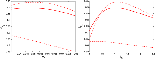
Figure 3: $\phi_{c_{3}}(\xi;\theta)$ as a function of $\theta$, for $\theta_{1}=\theta_{1}^{0}$ and $\theta_{3}=\theta_{3}^{0}$ (left) and $\theta_{1}=\theta_{1}^{0}$, $\theta_{2}=\theta_{2}^{0}$ (right); $\xi=\xi_{Ac_{3}-A}^{*}$ in dashed line, $\xi=\xi_{Ac_{3}-B}^{*}$ in dash–dotted line and $\xi=\xi_{ec_{3},\theta^{0}}^{*}$ in solid line.

Example 4.

For the same regression model (3), we change the value of $\theta^{0}$ and the set $\Theta$ and take $\theta^{0}=(0.773,0.214,2.09)^{\top}$ and $\Theta=[0,5]\times[0,5]\times[0,5]$, the values used by Kieffer and Walter (1998). With these values, from an investigation based on interval analysis, the authors report that for the 16-point design

$$\xi_{0}=\left\{\matrix{1&2&\cdots&16\vspace*{2pt}\cr 1/16&1/16&\cdots&1/16}\right\}$$

and the observations $\mathbf{y}$ given in their Table 13.1, the LS criterion $\|\mathbf{y}-\eta_{X}(\theta)\|^{2}$ has a global minimizer (the value we have taken here for $\theta^{0}$) and two other local minimizers in $\Theta$. The $D$- and $E$-optimal designs for $\theta^{0}$ are now given by

$$\xi_{D,\theta^{0}}^{*} \simeq \left\{\matrix{0.42&1.82&6.80\vspace*{2pt}\cr 1/3&1/3&1/3}\right\},$$

$$\xi_{E,\theta^{0}}^{*} \simeq \left\{\matrix{0.29&1.83&9.0\vspace*{2pt}\cr 0.4424&0.3318&0.2258}\right\}.$$

Using the same approach as in Example 3, with the grid $\mathscr{G}^{0}$ of (17)-(iii) obtained from a random Latin hypercube design with $10\mbox{,}000$ points in $\Theta$, we obtain

$$\xi_{eE,\theta^{0}}^{*}\simeq\left\{\matrix{0.38&2.26&7.91\vspace*{2pt}\cr 0.314&0.226&0.460}\right\}.$$

To compute an optimal design for $\phi_{eG}(\cdot)$, we consider the design space $\mathscr{X}=\{0,0.1,0.2,\ldots,16\}$ (with 161 points) and use the algorithm of Section 3.4 with the grid $\mathscr{G}^{0}$ of (17)-(iii) taken as a random Latin hypercube design with $10^{5}$ points. The same design space is used to evaluate $\phi_{eG}(\cdot)$ for the four designs above. For $\epsilon=10^{-10}$, the algorithm initialized at the uniform measure on $\mathscr{X}$ converges after 34 iterations in about 52 s and gives

$$\xi_{eG,\theta^{0}}^{*}\simeq\left\{\matrix{0.4&1.9&5.3&16\cr 0.278&0.258&0.244&0.22}\right\}.$$

Table 3: Performances of different designs and curvature measures at $\theta^{0}$ for the model (3) with $\theta^{0}=(0.773,0.214,2.09)^{\top}$ and $\Theta=[0,5]^{3}$; $\det^{1/3}=\phi_{D}(\xi)=\{\det[\mathbf{M}(\xi,\theta^{0})]\}^{1/3}$, $\lambda_{\min}=\phi_{E}(\xi)=\lambda_{\min}[\mathbf{M}(\xi,\theta^{0})]$. The optimal (maximum) values of the criteria are indicated in boldface

$\bolds{\xi}$	$\bolds{\det^{1/3}}$	$\bolds{\lambda_{\min}}$	$\bolds{\phi_{eE}}$	$\bolds{\phi_{eG}}$	$\bolds{C_{\mathrm{par}}}$	$\bolds{C_{\mathrm{int}}}$	$\bolds{C_{\mathrm{tot}}}$
$\xi_{0}$	$1.85\cdot 10^{-2}$	$1.92\cdot 10^{-4}$	$2.28\cdot 10^{-5}$	$5.66\cdot 10^{-3}$	$180.7$	$15.73$	$181.3$
$\xi_{D}^{*}$	$\mathbf{5\bolds{.}19\bolds{\cdot}10^{\bolds{-2}}}$	$1.69\cdot 10^{-3}$	$2.64\cdot 10^{-4}$	$6.70\cdot 10^{-2}$	$58.0$	$0$	$58.0$
$\xi_{E}^{*}$	$4.51\cdot 10^{-2}$	$\mathbf{2\bolds{.}04\bolds{\cdot}10^{\bolds{-3}}}$	$1.32\cdot 10^{-4}$	$7.95\cdot 10^{-2}$	$50.7$	$0$	$50.7$
$\xi_{eE}^{*}$	$4.73\cdot 10^{-2}$	$1.53\cdot 10^{-3}$	$\mathbf{2\bolds{.}92\bolds{\cdot}10^{\bolds{-4}}}$	0.114	$54.6$	$0$	$54.6$
$\xi_{eG}^{*}$	$4.11\cdot 10^{-2}$	$1.31\cdot 10^{-3}$	$1.69\cdot 10^{-4}$	0.244	$69.7$	$10.7$	$69.9$

The performances and curvature measures at $\theta^{0}$ of $\xi_{0}$, $\xi_{D}^{*}$, $\xi_{E}^{*}$, $\xi_{eE}^{*}$ and $\xi_{eG}^{*}$ are given in Table 3. The large intrinsic curvature for $\xi_{0}$, associated with the small values of $\phi_{eE}(\xi^{0})$ and $\phi_{eG}(\xi^{0})$, explains the presence of local minimizers for the LS criterion, and thus the possible difficulties for the estimation of $\theta$. The values of $\phi_{eE}(\cdot)$ and $\phi_{eG}(\cdot)$ reported in the table indicate that $\xi_{D}^{*}$, $\xi_{E}^{*}$, $\xi_{eE}^{*}$ or $\xi_{eG}^{*}$ would have caused less difficulties.

7 Further extensions and developments

7.1 An extra tuning parameter for a smooth transition to usual design criteria

The criterion $\phi_{eE}(\xi;\theta^{0})$ can be written as

$$\phi_{eE}\bigl{(}\xi;\theta^{0}\bigr{)}=\max\bigl{\{}\alpha\in\mathbb{R}\dvtx\bigl{\|}\eta(\cdot,\theta)-\eta\bigl{(}\cdot,\theta^{0}\bigr{)}\bigr{\|}_{\xi}^{2}\geq\alpha\bigl{\|}\theta-\theta^{0}\bigr{\|}^{2},$$

(21)

$$\hskip 218.0pt\mbox{for all }\theta\in\Theta\bigr{\}}.$$

Instead of giving the same importance to all $\theta$ whatever their distance to $\theta^{0}$, one may wish to introduce a saturation and reduce the importance given to those $\theta$ very far from $\theta^{0}$, that is, consider

$$\phi_{eE|K}\bigl{(}\xi;\theta^{0}\bigr{)}=\max\biggl{\{}\alpha\in\mathbb{R}\dvtx\bigl{\|}\eta(\cdot,\theta)-\eta\bigl{(}\cdot,\theta^{0}\bigr{)}\bigr{\|}_{\xi}^{2}\geq\alpha\frac{\|\theta-\theta^{0}\|^{2}}{1+K\|\theta-\theta^{0}\|^{2}},$$

(22)

$$\hskip 255.0pt\mbox{ for all }\theta\in\Theta\biggr{\}}$$

for some $K\geq 0$. Equivalently, $\phi_{eE|K}(\xi;\theta^{0})=\min_{\theta\in\Theta}H_{E|K}(\xi,\theta)$, with

$$H_{E|K}(\xi,\theta)=\bigl{\|}\eta(\cdot,\theta)-\eta\bigl{(}\cdot,\theta^{0}\bigr{)}\bigr{\|}_{\xi}^{2}\biggl{[}K+\frac{1}{\|\theta-\theta^{0}\|^{2}}\biggr{]}.$$

As in Section 3.1, we obtain $\phi_{eE|K}(\xi)=\lambda_{\min}[\mathbf{M}(\xi)]$ in a linear model and, for a nonlinear model with $\Theta=\mathscr{B}(\theta^{0},\rho)$, $\lim_{\rho\rightarrow 0}\phi_{eE|K}(\xi;\theta^{0})=\lambda_{\min}[\mathbf{M}(\xi,\theta^{0})]$ for any $K\geq 0$. Moreover, in a nonlinear model with no overlapping $\phi_{eE|K}(\xi;\theta^{0})$ can be made arbitrarily close to $\lambda_{\min}[\mathbf{M}(\xi,\theta^{0})]$ by choosing $K$ large enough, whereas choosing $K$ not too large ensures some protection against $\|\eta(\cdot,\theta)-\eta(\cdot,\theta^{0})\|_{\xi}$ being small for some $\theta$ far from $\theta^{0}$. Also, properties of $\phi_{eE}(\cdot)$ such as concavity, positive homogeneity, existence of directional derivatives; see Section 3.2, remain valid for $\phi_{eE|K}(\cdot)$, for any $K\geq 0$. The maximization of $\phi_{eE|K}(\cdot)$ forms a LP problem when both $\mathscr{X}$ and $\Theta$ are finite (see Section 3.3) and a relaxation procedure (cutting-plane method) can be used when $\Theta$ is a compact subset of $\mathbb{R}^{p}$; see Section 3.4.

A similar approach can be used with extended $c$- and $G$-optimality, which gives $\phi_{ec|K}(\xi)=\min_{\theta^{\prime}\in\Theta}H_{c|K}(\xi,\theta^{\prime})$ with

$$H_{c|K}(\xi,\theta)=\bigl{\|}\eta(\cdot,\theta)-\eta\bigl{(}\cdot,\theta^{0}\bigr{)}\bigr{\|}_{\xi}^{2}\biggl{[}K+\frac{1}{|g(\theta)-g(\theta^{0})|^{2}}\biggr{]}$$

and

$$\phi_{eG|K}(\xi)=\min_{\theta\in\Theta}\biggl{\{}\bigl{\|}\eta(\cdot,\theta)-\eta\bigl{(}\cdot,\theta^{0}\bigr{)}\bigr{\|}_{\xi}^{2}\biggl{[}K+\frac{1}{\max_{x\in\mathscr{X}}[\eta(x,\theta)-\eta(x,\theta^{0})]^{2}}\biggr{]}\biggr{\}},$$

for $K$ a positive constant.

7.2 Worst-case extended optimality criteria

The criterion defined by

$$\phi_{MeE}(\xi)=\min_{\theta^{0}\in\Theta}\phi_{eE}\bigl{(}\xi;\theta^{0}\bigr{)}=\min_{(\theta,\theta^{0})\in\Theta\times\Theta}H_{E}\bigl{(}\xi,\theta;\theta^{0}\bigr{)},$$

see (6), (5), accounts for the global behavior of $\eta(\cdot,\theta)$ for $\theta\in\Theta$ and obliterates the dependence on $\theta^{0}$ that is present in $\phi_{eE}(\xi;\theta^{0})$. The situation is similar to that in Section 3, excepted that we consider now the minimum of $H_{E}$ with respect to two vectors $\theta$ and $\theta^{0}$ in $\Theta\times\Theta$. All the developments in Section 3 obviously remain valid (concavity, existence of directional derivative, etc.), including the algorithmic solutions of Sections 3.3 and 3.4. The same is true for the worst-case versions of $\phi_{ec}(\cdot)$ and $\phi_{eG}(\cdot)$, respectively, defined by $\phi_{Mec}(\xi)=\min_{(\theta,\theta^{0})\in\Theta\times\Theta}H_{c}(\xi,\theta;\theta^{0})$, see (18), and by $\phi_{MeG}(\xi)=\min_{(\theta,\theta^{0})\in\Theta\times\Theta}\{\|\eta(\cdot,\theta)-\eta(\cdot,\theta^{0})\|_{\xi}^{2}/\max_{x\in\mathscr{X}}[\eta(x,\theta)-\eta(x,\theta^{0})]^{2}\}$, and for the worst-case versions of the extensions of previous section that include an additional tuning parameter $K$.

Note that the criterion $\phi_{MeE}(\cdot)$ may direct attention to a particularly pessimistic situation. Indeed, for $\Theta$ a compact set with nonempty interior and $\mu$ the Lebesgue measure on $\Theta$, one may have $\min_{\theta^{0}\in\Theta}\phi_{eE}(\xi;\theta^{0})=0$ for all designs $\xi$ although $\mu\{\theta^{0}\in\Theta\dvtx\phi_{eE}(\xi^{\prime};\theta^{0})>0\}=1$ for some design $\xi^{\prime}$. This corresponds to a situation where the model is structurally identifiable, in the sense that the property (2) is generic but is possibly false for $\theta$ in a subset of zero measure; see, for example, Walter (1987). Example 2 gives an illustration.

Example 2 ((Continued)).

When the three polynomial equations $\theta_{1}^{\prime}-{\theta_{1}^{\prime}}^{3}=\theta_{1}-\theta_{1}^{3}$, $\theta_{2}^{\prime}-{\theta_{2}^{\prime}}^{2}=\theta_{2}-\theta_{2}^{2}$, ${\theta_{1}^{\prime}}^{3}+{\theta_{2}^{\prime}}^{2}=\theta_{1}^{3}+\theta_{2}^{2}$ are satisfied, then $\eta(\mathbf{x},\theta^{\prime})=\eta(\mathbf{x},\theta)$ for all $\mathbf{x}$. Since these equations have solutions $\theta^{\prime}\neq\theta$ in $\Theta\times\Theta$, $\phi_{MeE}(\xi)=0$ for all $\xi\in\Xi$. On the other hand, $\max_{\xi\in\Xi}\phi_{eE}(\xi;\theta^{0})>0$ w.p.1. when $\theta^{0}$ is randomly drawn with a probability measure having a density with respect to the Lebesgue measure on $\Theta$.

In a less pessimistic version of worst-case extended $E$-optimality, we may thus consider a finite set $\Theta^{0}\subset\Theta$ for $\theta^{0}$, obtained for instance by random sampling in $\Theta$, and maximize $\min_{\theta^{0}\in\Theta^{0}}\phi_{eE}(\xi;\theta^{0})$.

8 Conclusions

Two essential ideas have been presented. First, classical optimality criteria can be extended in a mathematically consistent way to criteria that preserve a nonlinear model against overlapping, and at the same time retain the main features of classical criteria, especially concavity. Moreover, they coincide with their classical counterpart for linear models. Second, designs that are nearly optimal for those extended criteria can be obtained by standard linear programming solvers, supposing that the approximation of the feasible parameter space $\Theta$ by a finite set is acceptable. A relaxation method, equivalent to the cutting-plane algorithm, can be used when $\Theta$ is a compact set with nonempty interior. Linear constraints on the design can easily be taken into account. As a by-product, this also provides simple algorithmic procedures for the determination of $E$-, $c$- or $G$-optimal designs in linear models with linear cost constraints.

As it is usually the case for optimal design in nonlinear models, the extended-optimality criteria are local and depend on a guessed value $\theta^{0}$ for the model parameters. However, the construction of a globalized, worst-case version enjoying the same properties is straightforward (Section 7.2).

Finally, we recommend the following general procedure for optimal design in nonlinear regression. (i) Choose a parameter space $\Theta$ corresponding to the domain of interest for $\theta$, select (e.g., randomly) a finite subset $\Theta^{0}$ in the interior of $\Theta$; (ii) for each $\theta^{0}$ in $\Theta^{0}$ compute an optimal design $\xi_{eE,\theta^{0}}^{*}$ maximizing $\phi_{eE}(\xi;\theta^{0})$ and a $E$-optimal design $\xi_{E,\theta^{0}}^{*}$ maximizing $\phi_{E}(\xi;\theta^{0})=\lambda_{\min}\mathbf{M}(\xi,\theta^{0})$; (iii) if $\phi_{eE}(\xi_{eE,\theta^{0}}^{*};\theta^{0})$ is close enough to $\phi_{E}(\xi_{E,\theta^{0}}^{*};\theta^{0})$ for all $\theta^{0}$ in $\Theta^{0}$, one may consider that the risk of overlapping, or lack of identifiability in $\Theta$, is weak and classical optimal design that focuses on the precision of estimation can be used; otherwise, a design that maximizes $\min_{\theta^{0}\in\Theta^{0}}\phi_{eE}(\xi;\theta^{0})$ should be preferred. When the extended $G$-optimality criterion $\phi_{eG}(\cdot;\theta^{0})$ is substituted for $\phi_{eE}(\cdot;\theta^{0})$, the comparison in (iii) should be between $\phi_{eG}(\xi_{eG,\theta^{0}}^{*};\theta^{0})$ and $1/\operatorname{dim}(\theta)$, see Section 5. Extended $c$-optimality can be used when one is interested in estimating a (nonlinear) function of $\theta$, the comparison in (iii) should then be with $c$-optimality.

References

- Atkinson et al. (1993) {barticle}[author] \bauthor\bsnmAtkinson, \bfnmA. C.\binitsA. C., \bauthor\bsnmChaloner, \bfnmK.\binitsK., \bauthor\bsnmHerzberg, \bfnmA. M.\binitsA. M. and \bauthor\bsnmJuritz, \bfnmJ.\binitsJ. (\byear1993). \btitleOptimal experimental designs for properties of a compartmental model. \bjournalBiometrics \bvolume49 \bpages325–337.\bptokimsref\endbibitem
- Bates and Watts (1980) {barticle}[mr] \bauthor\bsnmBates, \bfnmDouglas M.\binitsD. M. and \bauthor\bsnmWatts, \bfnmDonald G.\binitsD. G. (\byear1980). \btitleRelative curvature measures of nonlinearity. \bjournalJ. R. Stat. Soc. Ser. B Stat. Methodol. \bvolume42 \bpages1–25. \bidissn=0035-9246, mr=0567196 \bptnotecheck related \bptokimsref\endbibitem
- Bonnans et al. (2006) {bbook}[mr] \bauthor\bsnmBonnans, \bfnmJ. Frédéric\binitsJ. F., \bauthor\bsnmGilbert, \bfnmJ. Charles\binitsJ. C., \bauthor\bsnmLemaréchal, \bfnmClaude\binitsC. and \bauthor\bsnmSagastizábal, \bfnmClaudia A.\binitsC. A. (\byear2006). \btitleNumerical Optimization: Theoretical and Practical Aspects, \bedition2nd ed. \bpublisherSpringer, \blocationBerlin. \bidmr=2265882 \bptokimsref\endbibitem
- Chavent (1983) {barticle}[mr] \bauthor\bsnmChavent, \bfnmG.\binitsG. (\byear1983). \btitleLocal stability of the output least square parameter estimation technique. \bjournalMat. Apl. Comput. \bvolume2 \bpages3–22. \bidissn=0101-8205, mr=0699367 \bptokimsref\endbibitem
- Chavent (1990) {bincollection}[author] \bauthor\bsnmChavent, \bfnmG.\binitsG. (\byear1990). \btitleA new sufficient condition for the well-posedness of nonlinear least square problems arising in identification and control. In \bbooktitleAnalysis and Optimization of Systems (\beditor\bfnmA.\binitsA. \bsnmBensoussan and \beditor\bfnmJ. L.\binitsJ. L. \bsnmLions, eds.). \bseriesLecture Notes in Control and Inform. Sci. \bvolume144 \bpages452–463. \bpublisherSpringer, \blocationBerlin. \bidmr=1070759 \bptokimsref\endbibitem
- Chavent (1991) {barticle}[mr] \bauthor\bsnmChavent, \bfnmGuy\binitsG. (\byear1991). \btitleNew sizecurvature conditions for strict quasiconvexity of sets. \bjournalSIAM J. Control Optim. \bvolume29 \bpages1348–1372. \biddoi=10.1137/0329069, issn=0363-0129, mr=1132186 \bptokimsref\endbibitem
- Clyde and Chaloner (2002) {barticle}[mr] \bauthor\bsnmClyde, \bfnmMerlise\binitsM. and \bauthor\bsnmChaloner, \bfnmKathryn\binitsK. (\byear2002). \btitleConstrained design strategies for improving normal approximations in nonlinear regression problems. \bjournalJ. Statist. Plann. Inference \bvolume104 \bpages175–196. \biddoi=10.1016/S0378-3758(01)00239-7, issn=0378-3758, mr=1900525 \bptokimsref\endbibitem
- Dem’yanov and Malozemov (1974) {bbook}[author] \bauthor\bsnmDem’yanov, \bfnmV. F.\binitsV. F. and \bauthor\bsnmMalozemov, \bfnmV. N.\binitsV. N. (\byear1974). \btitleIntroduction to Minimax. \bpublisherDover, \blocationNew York. \bptokimsref\endbibitem
- Demidenko (1989) {bbook}[mr] \bauthor\bsnmDemidenko, \bfnmE. Z.\binitsE. Z. (\byear1989). \btitleOptimizatsiya i Regressiya. \bpublisherNauka, \blocationMoscow. \bidmr=1007832 \bptokimsref\endbibitem
- Demidenko (2000) {barticle}[mr] \bauthor\bsnmDemidenko, \bfnmEugene\binitsE. (\byear2000). \btitleIs this the least squares estimate? \bjournalBiometrika \bvolume87 \bpages437–452. \biddoi=10.1093/biomet/87.2.437, issn=0006-3444, mr=1782489 \bptokimsref\endbibitem
- Fedorov (1972) {bbook}[mr] \bauthor\bsnmFedorov, \bfnmV. V.\binitsV. V. (\byear1972). \btitleTheory of Optimal Experiments. \bpublisherAcademic Press, \blocationNew York. \bidmr=0403103 \bptokimsref\endbibitem
- Fedorov and Hackl (1997) {bbook}[mr] \bauthor\bsnmFedorov, \bfnmValerii V.\binitsV. V. and \bauthor\bsnmHackl, \bfnmPeter\binitsP. (\byear1997). \btitleModel-Oriented Design of Experiments. \bseriesLecture Notes in Statistics \bvolume125. \bpublisherSpringer, \blocationNew York. \biddoi=10.1007/978-1-4612-0703-0, mr=1454123 \bptokimsref\endbibitem
- Fedorov and Leonov (2014) {bbook}[mr] \bauthor\bsnmFedorov, \bfnmValerii V.\binitsV. V. and \bauthor\bsnmLeonov, \bfnmSergei L.\binitsS. L. (\byear2014). \btitleOptimal Design for Nonlinear Response Models. \bpublisherCRC Press, \blocationBoca Raton, FL. \bidmr=3113978 \bptokimsref\endbibitem
- Gauchi and Pázman (2006) {barticle}[mr] \bauthor\bsnmGauchi, \bfnmJ.-P.\binitsJ.-P. and \bauthor\bsnmPázman, \bfnmA.\binitsA. (\byear2006). \btitleDesigns in nonlinear regression by stochastic minimization of functionals of the mean square error matrix. \bjournalJ. Statist. Plann. Inference \bvolume136 \bpages1135–1152. \biddoi=10.1016/j.jspi.2004.08.015, issn=0378-3758, mr=2181993 \bptokimsref\endbibitem
- Hamilton and Watts (1985) {barticle}[mr] \bauthor\bsnmHamilton, \bfnmDavid C.\binitsD. C. and \bauthor\bsnmWatts, \bfnmDonald G.\binitsD. G. (\byear1985). \btitleA quadratic design criterion for precise estimation in nonlinear regression models. \bjournalTechnometrics \bvolume27 \bpages241–250. \biddoi=10.2307/1269705, issn=0040-1706, mr=0797562 \bptokimsref\endbibitem
- Harville (1997) {bbook}[author] \bauthor\bsnmHarville, \bfnmD. A.\binitsD. A. (\byear1997). \btitleMatrix Algebra from a Statistician’s Perspective. \bpublisherSpringer, \blocationHeidelberg. \bidmr=1467237 \bptokimsref\endbibitem
- Kelley (1960) {barticle}[mr] \bauthor\bsnmKelley, \bfnmJ. E.\binitsJ. E. \bsuffixJr. (\byear1960). \btitleThe cutting-plane method for solving convex programs. \bjournalJ. Soc. Indust. Appl. Math. \bvolume8 \bpages703–712. \bidmr=0118538 \bptokimsref\endbibitem
- Kiefer and Wolfowitz (1960) {barticle}[mr] \bauthor\bsnmKiefer, \bfnmJ.\binitsJ. and \bauthor\bsnmWolfowitz, \bfnmJ.\binitsJ. (\byear1960). \btitleThe equivalence of two extremum problems. \bjournalCanad. J. Math. \bvolume12 \bpages363–366. \bidissn=0008-414X, mr=0117842 \bptokimsref\endbibitem
- Kieffer and Walter (1998) {bincollection}[mr] \bauthor\bsnmKieffer, \bfnmM.\binitsM. and \bauthor\bsnmWalter, \bfnmE.\binitsE. (\byear1998). \btitleInterval analysis for guaranteed nonlinear parameter estimation. In \bbooktitleMODA 5—Advances in Model-Oriented Data Analysis and Experimental Design (Marseilles, 1998) (\beditor\bfnmA. C.\binitsA. C. \bsnmAtkinson, \beditor\bfnmL.\binitsL. \bsnmPronzato and \beditor\bfnmH. P.\binitsH. P. \bsnmWynn, eds.) \bpages115–125. \bpublisherPhysica, \blocationHeidelberg. \bidmr=1652219 \bptokimsref\endbibitem
- Lemaréchal, Nemirovskii and Nesterov (1995) {barticle}[mr] \bauthor\bsnmLemaréchal, \bfnmClaude\binitsC., \bauthor\bsnmNemirovskii, \bfnmArkadii\binitsA. and \bauthor\bsnmNesterov, \bfnmYurii\binitsY. (\byear1995). \btitleNew variants of bundle methods. \bjournalMath. Program. \bvolume69 \bpages111–147. \biddoi=10.1007/BF01585555, issn=0025-5610, mr=1354434 \bptokimsref\endbibitem
- Nesterov (2004) {bbook}[mr] \bauthor\bsnmNesterov, \bfnmYurii\binitsY. (\byear2004). \btitleIntroductory Lectures on Convex Optimization: A Basic Course. \bseriesApplied Optimization \bvolume87. \bpublisherKluwer Academic, \blocationBoston, MA. \biddoi=10.1007/978-1-4419-8853-9, mr=2142598 \bptokimsref\endbibitem
- Pázman (1984) {barticle}[mr] \bauthor\bsnmPázman, \bfnmA.\binitsA. (\byear1984). \btitleNonlinear least squares—uniqueness versus ambiguity. \bjournalMath. Operationsforsch. Statist. Ser. Statist. \bvolume15 \bpages323–336. \biddoi=10.1080/02331888408801771, issn=0323-3944, mr=0756337 \bptokimsref\endbibitem
- Pázman (1993) {bbook}[author] \bauthor\bsnmPázman, \bfnmA.\binitsA. (\byear1993). \btitleNonlinear Statistical Models. \bpublisherKluwer, \blocationDordrecht. \bptokimsref\endbibitem
- Pázman and Pronzato (1992) {barticle}[mr] \bauthor\bsnmPázman, \bfnmAndrej\binitsA. and \bauthor\bsnmPronzato, \bfnmLuc\binitsL. (\byear1992). \btitleNonlinear experimental design based on the distribution of estimators. \bjournalJ. Statist. Plann. Inference \bvolume33 \bpages385–402. \biddoi=10.1016/0378-3758(92)90007-F, issn=0378-3758, mr=1200655 \bptokimsref\endbibitem
- Pronzato (2009) {barticle}[mr] \bauthor\bsnmPronzato, \bfnmLuc\binitsL. (\byear2009). \btitleOn the regularization of singular -optimal designs. \bjournalMath. Slovaca \bvolume59 \bpages611–626. \biddoi=10.2478/s12175-009-0151-2, issn=0139-9918, mr=2557313 \bptokimsref\endbibitem
- Pronzato, Huang and Walter (1991) {binproceedings}[author] \bauthor\bsnmPronzato, \bfnmL.\binitsL., \bauthor\bsnmHuang, \bfnmC. Y.\binitsC. Y. and \bauthor\bsnmWalter, \bfnmE.\binitsE. (\byear1991). \btitleNonsequential -optimal design for model discrimination: New algorithms. In \bbooktitleProc. PROBASTAT’91 (\beditor\bfnmA.\binitsA. \bsnmPázman and \beditor\bfnmJ.\binitsJ. \bsnmVolaufová, eds.) \bpages130–136. \bpublisherMathematical Institute of the Slovak Academy of Sciences, \blocationBratislava. \bptokimsref\endbibitem
- Pronzato and Pázman (1994) {barticle}[mr] \bauthor\bsnmPronzato, \bfnmLuc\binitsL. and \bauthor\bsnmPázman, \bfnmAndrej\binitsA. (\byear1994). \btitleSecond-order approximation of the entropy in nonlinear least-squares estimation. \bjournalKybernetika (Prague) \bvolume30 \bpages187–198. \bidissn=0023-5954, mr=1283494 \bptnotecheck related \bptokimsref\endbibitem
- Pronzato and Pázman (2013) {bbook}[mr] \bauthor\bsnmPronzato, \bfnmLuc\binitsL. and \bauthor\bsnmPázman, \bfnmAndrej\binitsA. (\byear2013). \btitleDesign of Experiments in Nonlinear Models: Asymptotic Normality, Optimality Criteria and Small-Sample Properties. \bseriesLecture Notes in Statistics \bvolume212. \bpublisherSpringer, \blocationNew York. \biddoi=10.1007/978-1-4614-6363-4, mr=3058804 \bptokimsref\endbibitem
- Pukelsheim (1993) {bbook}[author] \bauthor\bsnmPukelsheim, \bfnmF.\binitsF. (\byear1993). \btitleOptimal Experimental Design. \bpublisherWiley, \blocationNew York. \bptokimsref\endbibitem
- Ratkowsky (1983) {bbook}[author] \bauthor\bsnmRatkowsky, \bfnmD. A.\binitsD. A. (\byear1983). \btitleNonlinear Regression Modelling. \bpublisherDekker, \blocationNew York. \bptokimsref\endbibitem
- Shimizu and Aiyoshi (1980) {barticle}[mr] \bauthor\bsnmShimizu, \bfnmKiyotaka\binitsK. and \bauthor\bsnmAiyoshi, \bfnmEitaro\binitsE. (\byear1980). \btitleNecessary conditions for min-max problems and algorithms by a relaxation procedure. \bjournalIEEE Trans. Automat. Control \bvolume25 \bpages62–66. \biddoi=10.1109/TAC.1980.1102226, issn=0018-9286, mr=0561341 \bptokimsref\endbibitem
- Silvey (1980) {bbook}[mr] \bauthor\bsnmSilvey, \bfnmSamuel David\binitsS. D. (\byear1980). \btitleOptimal Design. \bpublisherChapman & Hall, \blocationLondon. \bidmr=0606742 \bptokimsref\endbibitem
- Tang (1993) {barticle}[mr] \bauthor\bsnmTang, \bfnmBoxin\binitsB. (\byear1993). \btitleOrthogonal array-based Latin hypercubes. \bjournalJ. Amer. Statist. Assoc. \bvolume88 \bpages1392–1397. \bidissn=0162-1459, mr=1245375 \bptokimsref\endbibitem
- Walter (1987) {bbook}[author] \beditor\bsnmWalter, \bfnmE.\binitsE., ed. (\byear1987). \btitleIdentifiability of Parametric Models. \bpublisherPergamon Press, \blocationOxford. \bptokimsref\endbibitem
- Walter and Pronzato (1995) {bincollection}[mr] \bauthor\bsnmWalter, \bfnmE.\binitsE. and \bauthor\bsnmPronzato, \bfnmL.\binitsL. (\byear1995). \btitleIdentifiabilities and nonlinearities. In \bbooktitleNonlinear Systems, Vol. 1 (\beditor\bfnmA. J.\binitsA. J. \bsnmFossard and \beditor\bfnmD.\binitsD. \bsnmNormand-Cyrot, eds.) \bpages111–143. \bpublisherChapman & Hall, \blocationLondon. \bidmr=1359307 \bptokimsref\endbibitem