Learning Algorithms for Second-Price Auctions with Reserve

Abstract

Second-price auctions with reserve play a critical role in the revenue of modern search engine and popular online sites since the revenue of these companies often directly depends on the outcome of such auctions. The choice of the reserve price is the main mechanism through which the auction revenue can be influenced in these electronic markets. We cast the problem of selecting the reserve price to optimize revenue as a learning problem and present a full theoretical analysis dealing with the complex properties of the corresponding loss function. We further give novel algorithms for solving this problem and report the results of several experiments in both synthetic and real data demonstrating their effectiveness.

1 Introduction

Over the past few years, advertisement has gradually moved away from the traditional printed promotion to the more tailored and directed online publicity. The advantages of online advertisement are clear: since most modern search engine and popular online site companies such as as Microsoft, Facebook, Google, eBay, or Amazon, may collect information about the users’ behavior, advertisers can better target the population sector their brand is intended for.

More recently, a new method for selling advertisements has gained momentum. Unlike the standard contracts between publishers and advertisers where some amount of impressions is required to be fulfilled by the publisher, an Ad Exchange works in a way similar to a financial exchange where advertisers bid and compete between each other for an ad slot. The winner then pays the publisher and his ad is displayed.

The design of such auctions and their properties are crucial since they generate a large fraction of the revenue of popular online sites. These questions have motivated extensive research on the topic of auctioning in the last decade or so, particularly in the theoretical computer science and economic theory communities. Much of this work has focused on the analysis of mechanism design, either to prove some useful property of an existing auctioning mechanism, to analyze its computational efficiency, or to search for an optimal revenue maximization truthful mechanism (see (Muthukrishnan, 2009) for a good discussion of key research problems related to Ad Exchange and references to a fast growing literature therein).

One important problem is that of determining an auction mechanism that achieves optimal revenue Muthukrishnan (2009). In the ideal scenario where the valuation of the bidders is drawn i.i.d. from a given distribution, this is known to be achievable (see for example (Myerson, 1981)). But, even good approximations of such distributions are not known in practice. Game theoretical approaches to the design of auctions have given a series of interesting results including (Riley and Samuelson, 1981; Milgrom and Weber, 1982; Myerson, 1981; Nisan et al., 2007), all of them based on some assumptions about the distribution of the bidders, e.g., the monotone hazard rate assumption.

The results of the recent publications have nevertheless set the basis for most Ad Exchanges in practice: the mechanism widely adopted for selling ad slots is that of a Vickrey auction (Vickrey, 1961) or second-price auction with reserve price $r$ (Easley and Kleinberg, 2010). In such auctions, the winning bidder (if any) pays the maximum of the second-place bid and the reserve price $r$. The reserve price can be set by the publisher or automatically by the exchange. The popularity of these auctions relies on the fact that they are incentive compatible, i.e., bidders bid exactly what they are willing to pay. It is clear that the revenue of the publisher depends greatly on how the reserve price is set: if set too low, the winner of the auction might end up paying only a small amount, even if his bid was really high; on the other hand, if it is set too high, then bidders may not bid higher than the reserve price and the ad slot will not be sold.

We propose a machine learning approach to the problem of determining the reserve price to optimize revenue in such auctions. The general idea is to leverage the information gained from past auctions to predict a beneficial reserve price. Since every transaction on an Exchange is logged, it is natural to seek to exploit that data. This could be used to estimate the probability distribution of the bidders, which can then be used indirectly to come up with the optimal reserve price (Myerson, 1981; Ostrovsky and Schwarz, 2011). Instead, we will seek a discriminative method making use of the loss function related to the problem and taking advantage of existing user features.

Machine learning methods have already been used for the related problems of designing incentive compatible auction mechanisms Balcan et al. (2008); Blum et al. (2004), for algorithmic bidding Langford et al. (2010); Amin et al. (2012), and even for predicting bid landscapes Cui et al. (2011). Another closely related problem for which machine learning solutions have been proposed is that of revenue optimization for sponsored search ads and click through rate predictions Zhu et al. (2009); He et al. (2013); Devanur and Kakade (2009). But, to our knowledge, no prior work has used historical data in combination with user features for the sole purpose of revenue optimization in this context. In fact, the only publications we are aware of that are directly related to our objective are (Ostrovsky and Schwarz, 2011) and the interesting work of Cesa-Bianchi et al. (2013) which considers a more general case than (Ostrovsky and Schwarz, 2011). The scenario studied by Cesa-Bianchi et al. is that of censored information, which motivates their use of a regret minimization algorithm to optimize the revenue of the seller. Our analysis assumes instead access to full information. We argue that this is a more realistic scenario since most companies do in fact have access to the full historical data.

The learning scenario we consider is more general since it includes the use of features, as is standard in supervised learning. Since user information is sent to advertisers and bids are made based on this information, it is only natural to include user features in our learning solution. A special case of our analysis coincides with the no-feature scenario considered by Cesa-Bianchi et al. (2013), assuming full information. But, our results further extend those of this paper even in that scenario. In particular, we present an $O(m\log m)$ algorithm for solving a key optimization problem used as a subroutine by the authors, for which they do not seem to give an algorithm. We also do not require an i.i.d. assumption about the bidders, although this is needed in (Cesa-Bianchi et al., 2013) in order to deal with censored information only.

The theoretical and algorithmic analysis of this learning problem raises several non-trivial technical issues. This is because, unlike some common problems in machine learning, here, the use of a convex surrogate loss cannot be successful. Instead, we must derive an alternative non-convex surrogate requiring novel theoretical guarantees (Section 3) and a new algorithmic solution (Section 4). We present a detailed analysis of possible surrogate losses and select a continuous loss that we prove to be calibrated and for which we give generalization bounds. This leads to an optimization problem cast as a DC-programming problem whose solutions are examined in detail: we first present an efficient combinatorial algorithm for solving that optimization in the no-feature case, next we combine that solution with the DC algorithm (DCA) Tao and An (1998) to solve the general case. Section 5 reports the results of our experiments with synthetic data in both the no-feature case and the general case as well as on data collected from eBay. We first introduce the problem of selecting the reserve price to optimize revenue and cast it as a learning problem (Section 2).

2 Reserve price selection problem

As already discussed, the choice of the reserve price $r$ is the main mechanism through which a seller can influence the auction revenue. To specify the results of a second-price auction we need only the vector of first and second highest bids which we denote by ${\mathbf{b}}=(b^{(1)},b^{(2)})\in\mathcal{B}\subset\mathbb{R}_{+}^{2}$. For a given reserve price $r$ and bid pair ${\mathbf{b}}$, the revenue of an auction is given by

$$\mathrm{Revenue}(r,{\mathbf{b}})=b^{(2)}\mathds{1}_{r<b^{(2)}}+r\mathds{1}_{b^{(2)}\leq r\leq b^{(1)}}.$$ (1)

The simplest setup is one where there are no features associated with the auction. In that case, the objective is to select $r$ to optimize the expected revenue, which can be expressed as follows:

$$\operatorname*{\mathbb{E}}_{{\mathbf{b}}}[\mathrm{Revenue}(r,{\mathbf{b}})] =\operatorname*{\mathbb{E}}_{b^{(2)}}[b^{(2)}\mathds{1}_{r<b^{(2)}}]+r\operatorname*{\mathbb{P}}[b^{(2)}\leq r\leq b^{(1)}]$$

$$=\int_{0}^{+\infty}\operatorname*{\mathbb{P}}[b^{(2)}\mathds{1}_{r<b^{(2)}}>t]\,dt+r\operatorname*{\mathbb{P}}[b^{(2)}\leq r\leq b^{(1)}]$$

$$=\int_{0}^{r}\operatorname*{\mathbb{P}}[r<b^{(2)}]\,dt+\int_{r}^{\infty}\operatorname*{\mathbb{P}}[b^{(2)}>t]dt+r\operatorname*{\mathbb{P}}[b^{(2)}\leq r\leq b^{(1)}]$$

$$=\int_{r}^{\infty}\operatorname*{\mathbb{P}}[b^{(2)}>t]\,dt+r(\operatorname*{\mathbb{P}}[b^{(2)}>r]+1-\operatorname*{\mathbb{P}}[b^{(2)}>r]-\operatorname*{\mathbb{P}}[b^{(1)}<r])$$

$$=\int_{r}^{\infty}\operatorname*{\mathbb{P}}[b^{(2)}>t]\,dt+r\operatorname*{\mathbb{P}}[b^{(1)}\geq r].$$

A similar derivation is given by Cesa-Bianchi et al. (2013). In fact, this expression is precisely the one optimized by these authors. If we now associate with each auction a feature vector ${\mathbf{x}}\in\mathcal{X}$, the so-called public information, and set the reserve price to $h({\mathbf{x}})$, where $h\colon\mathcal{X}\to\mathbb{R}_{+}$ is our reserve price hypothesis function, the problem can be formulated as that of selecting out of some hypothesis set $H$ a hypothesis $h$ with large expected revenue:

$$\operatorname*{\mathbb{E}}_{({\mathbf{x}},{\mathbf{b}})\sim D}[\mathrm{Revenue}(h({\mathbf{x}}),{\mathbf{b}})],$$ (2)

where $D$ is the unknown distribution according to which the pairs $({\mathbf{x}},{\mathbf{b}})$ are drawn. Instead of the revenue, we will consider a loss function $L$ defined for all $(r,{\mathbf{b}})$ by $L(r,{\mathbf{b}})=-\mathrm{Revenue}(r,{\mathbf{b}})$, and will seek a hypothesis $h$ with small expected loss $\mathcal{L}(h):=\operatorname*{\mathbb{E}}_{({\mathbf{x}},{\mathbf{b}})\sim D}[L(h({\mathbf{x}}),{\mathbf{b}})]$. As in standard supervised learning scenarios, we assume access to a training sample $S=(({\mathbf{x}}_{1},{\mathbf{b}}_{1}),\ldots,({\mathbf{x}}_{m},{\mathbf{b}}_{m}))$ of size $m\geq 1$ drawn i.i.d. according to $D$ and denote by $\widehat{\mathcal{L}}_{S}(h)$ the empirical loss $\frac{1}{m}\sum_{i=1}^{m}L(h({\mathbf{x}}_{i},{\mathbf{b}}_{i})$. In the next sections, we present a detailed study of this learning problem.

3 Learning guarantees

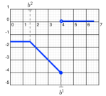
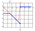
(a)	(b)

Figure 1: (a) Plot of the loss function $r\mapsto L(r,{\mathbf{b}})$ for fixed values of $b^{(1)}$ and $b^{(2)}$; (b) piecewise linear convex surrogate loss.

To derive generalization bounds for the learning problem formulated in the previous section, we need to analyze the complexity of the family of functions $L_{H}$ mapping $\mathcal{X}\times\mathcal{B}$ to $\mathbb{R}$ defined by $L_{H}=\{({\mathbf{x}},{\mathbf{b}})\mapsto L(h({\mathbf{x}}),{\mathbf{b}})\colon h\in H\}$. The loss function $L$ is neither Lipschitz continuous nor convex (see Figure 1). To analyze its complexity, we decompose $L$ as a sum of two loss functions $l_{1}$ and $l_{2}$ with more convenient properties. We have $L=l_{1}+l_{2}$ with $l_{1}$ and $l_{2}$ defined for all $(r,{\mathbf{b}})\in\mathbb{R}\times\mathcal{B}$ by

$$l_{1}(r,{\mathbf{b}}) =-b^{(2)}\mathds{1}_{r<b^{(2)}}-r\mathds{1}_{b^{(2)}\leq r\leq b^{(1)}}-b^{(1)}\mathds{1}_{r>b^{(1)}}$$

$$l_{2}(r,{\mathbf{b}}) =b^{(1)}\mathds{1}_{r>b^{(1)}}.$$

Note that for a fixed ${\mathbf{b}}$, the function $r\mapsto l_{1}(r,{\mathbf{b}})$ is $1$-Lipschitz since the slope of the lines defining the function is at most $1$. We will consider the corresponding family of loss functions: $l_{1H}=\{({\mathbf{x}},{\mathbf{b}})\mapsto l_{1}(h({\mathbf{x}}),{\mathbf{b}})\colon h\in H\}$ and $l_{2H}=\{({\mathbf{x}},{\mathbf{b}})\mapsto l_{2}(h({\mathbf{x}}),{\mathbf{b}})\colon h\in H\}$ and use the notions of pseudo-dimension as well as empirical and average Rademacher complexity. The pseudo-dimension is a standard complexity measure (Pollard, 1984) extending the notion of VC-dimension to real-valued functions (see also (Mohri et al., 2012)). For a family of functions $G$ and finite sample $S=(z_{1},\ldots,z_{m})$ of size $m$, the empirical Rademacher complexity is defined by $\widehat{\mathfrak{R}}_{S}(G)=\operatorname*{\mathbb{E}}_{\boldsymbol{\sigma}}\left[\sup_{g\in G}\frac{1}{m}\sum_{i=1}^{m}\sigma_{i}g(z_{i})\right]$, where ${\boldsymbol{\sigma}}=(\sigma_{1},\ldots,\sigma_{m})^{\top}$, with $\sigma_{i}$s independent uniform random variables taking values in $\{-1,+1\}$. The Rademacher complexity of $G$ is defined as $\mathfrak{R}_{m}(G)=\operatorname*{\mathbb{E}}_{S\sim D^{m}}[\widehat{\mathfrak{R}}_{S}(G)]$.

In order to bound the complexity of $L_{H}$ we will first bound the complexity of the family of loss functions $l_{1H}$ and $l_{2H}$.

Proposition 1

For any hypothesis set $H$ and any sample $S=(({\mathbf{x}}_{1},{\mathbf{b}}_{1}),\ldots,({\mathbf{x}}_{m},{\mathbf{b}}_{m}))$, the empirical Rademacher complexity of $l_{1H}$ can be bounded as follows:

$$\widehat{\mathfrak{R}}_{S}(l_{1H})\leq\widehat{\mathfrak{R}}_{S}(H).$$

Proof  By definition of the empirical Rademacher complexity, we can write

$$\widehat{\mathfrak{R}}_{S}(l_{1H})=\frac{1}{m}\operatorname*{\mathbb{E}}_{{\boldsymbol{\sigma}}}\left[\sup_{h\in H}\sum_{i=1}^{m}\sigma_{i}l_{1}(h({\mathbf{x}}_{i}),{\mathbf{b}}_{i})\right]=\frac{1}{m}\operatorname*{\mathbb{E}}_{{\boldsymbol{\sigma}}}\left[\sup_{h\in H}\sum_{i=1}^{m}\sigma_{i}(\psi_{i}\circ h)({\mathbf{x}}_{i})\right],$$

where, for all $i\in[1,m]$, $\psi_{i}$ is the function defined by $\psi_{i}\colon r\mapsto l_{1}(r,{\mathbf{b}}_{i})$. For any $i\in[1,m]$, $\psi_{i}$ is $1$-Lipschitz, thus, by the contraction lemma 18, we have the inequality $\widehat{\mathfrak{R}}_{S}(l_{1H})\leq\frac{1}{m}\operatorname*{\mathbb{E}}_{{\boldsymbol{\sigma}}}[\sup_{h\in H}\sum_{i=1}^{m}\sigma_{i}h({\mathbf{x}}_{i})]=\widehat{\mathfrak{R}}_{S}(H)$.  

Proposition 2

Let $M=\sup_{{\mathbf{b}}\in\mathcal{B}}b^{(1)}$. Then, for any hypothesis set $H$ with pseudo-dimension $d=\text{Pdim}(H)$ and any sample $S=(({\mathbf{x}}_{1},{\mathbf{b}}_{1}),\ldots,({\mathbf{x}}_{m},{\mathbf{b}}_{m}))$, the empirical Rademacher complexity of $l_{2H}$ can be bounded as follows:

$$\widehat{\mathfrak{R}}_{S}(l_{2H})\leq\sqrt{\frac{2d\log\frac{em}{d}}{m}}.$$

Proof  By definition of the empirical Rademacher complexity, we can write

$$\widehat{\mathfrak{R}}_{S}(l_{2H})=\frac{1}{m}\operatorname*{\mathbb{E}}_{{\boldsymbol{\sigma}}}\Big{[}\sup_{h\in H}\sum_{i=1}^{m}\sigma_{i}b^{(1)}_{i}\mathds{1}_{h({\mathbf{x}}_{i})>b^{(1)}_{i}}\Big{]}=\frac{1}{m}\operatorname*{\mathbb{E}}_{{\boldsymbol{\sigma}}}\Big{[}\sup_{h\in H}\sum_{i=1}^{m}\sigma_{i}\Psi_{i}(\mathds{1}_{h({\mathbf{x}}_{i})>b^{(1)}_{i}})\Big{]},$$

where for all $i\in[1,m]$, $\Psi_{i}$ is the $M$-Lipschitz function $x\mapsto b^{(1)}_{i}x$. Thus, by Lemma 18 combined with Massart’s lemma (see for example Mohri et al. (2012)), we can write

$$\widehat{\mathfrak{R}}_{S}(l_{2H})\leq\frac{M}{m}\operatorname*{\mathbb{E}}_{{\boldsymbol{\sigma}}}\Big{[}\sup_{h\in H}\sum_{i=1}^{m}\sigma_{i}\mathds{1}_{h({\mathbf{x}}_{i})>b^{(1)}_{i}}\Big{]}\leq M\sqrt{\frac{2d^{\prime}\log\frac{em}{d^{\prime}}}{m}},$$

where $d^{\prime}=\text{VCdim}(\{({\mathbf{x}},{\mathbf{b}})\mapsto\mathds{1}_{h({\mathbf{x}})-b^{(1)}>0}\colon({\mathbf{x}},{\mathbf{b}})\in\mathcal{X}\times\mathcal{B}\})$. Since the second bid component $b^{(2)}$ plays no role in this definition, $d^{\prime}$ coincides with $\text{VCdim}(\{({\mathbf{x}},b^{(1)})\mapsto\mathds{1}_{h({\mathbf{x}})-b^{(1)}>0}\colon({\mathbf{x}},b^{(1)})\in\mathcal{X}\times\mathcal{B}_{1}\})$, where $\mathcal{B}_{1}$ is the projection of $\mathcal{B}\subseteq\mathbb{R}^{2}$ onto its first component, and is upper-bounded by $\text{VCdim}(\{({\mathbf{x}},t)\mapsto\mathds{1}_{h({\mathbf{x}})-t>0}\colon({\mathbf{x}},t)\in\mathcal{X}\times\mathbb{R}\})$, that is, the pseudo-dimension of $H$.  

Theorem 3

Let $M=\sup_{{\mathbf{b}}\in\mathcal{B}}b^{(1)}$ and let $H$ be a hypothesis set with pseudo-dimension $d=\text{Pdim}(H)$. Then, for any $\delta>0$, with probability at least $1-\delta$ over the choice of a sample $S$ of size $m$, the following inequality holds for all $h\in H$:

$$\mathcal{L}(h)\leq\widehat{\mathcal{L}}_{S}(h)+2\mathfrak{R}_{m}(H)+2M\sqrt{\frac{2d\log\frac{em}{d}}{m}}+M\sqrt{\frac{\log\frac{1}{\delta}}{2m}}.$$

Proof  By a standard property of the Rademacher complexity, since $L=l_{1}+l_{2}$, the following inequality holds: $\mathfrak{R}_{m}(L_{H})\leq\mathfrak{R}_{m}(l_{1H})+\mathfrak{R}_{m}(l_{2H})$. Thus, in view of Propositions 1 and 2, the Rademacher complexity of $L_{H}$ can be bounded via

$$\mathfrak{R}_{m}(L_{H})\leq\mathfrak{R}_{m}(H)+M\sqrt{\frac{2d\log\frac{em}{d}}{m}}.$$

The result then follows by the application of a standard Rademacher complexity bound (Koltchinskii and Panchenko, 2002).  
This learning bound invites us to consider an algorithm seeking $h\!\in\!H$ to minimize the empirical loss $\widehat{\mathcal{L}}_{S}(h)$, while controlling the complexity (Rademacher complexity and pseudo-dimension) of the hypothesis set $H$. However, as in the familiar case of binary classification, in general, minimizing this empirical loss is a computationally hard problem. Thus, in the next section, we study the question of using a surrogate loss instead of the original loss $L$.

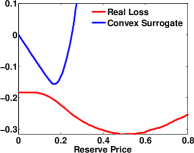
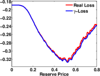
(a)	(b)

Figure 2: Comparison of the sum of real losses $\sum_{i=1}^{m}L(\cdot,{\mathbf{b}}_{i})$ for $m=500$ versus two different surrogates. (a) Sum of convex surrogate losses: the minimizer significantly differs from that of the sum of the original losses. (b) The surrogate loss sum $\sum_{i=1}^{m}L_{\gamma}(\cdot,{\mathbf{b}}_{i})$ for $\gamma=.02$

3.1 Surrogate loss

As pointed out earlier, the loss function $L$ does not admit some common useful properties: for any fixed ${\mathbf{b}}$, $L(\cdot,{\mathbf{b}})$ is not differentiable at two points, is not convex, and is not Lipschitz, in fact it is discontinuous. For any fixed ${\mathbf{b}}$, $L(\cdot,{\mathbf{b}})$ is quasi-convex, a property that is often desirable since there exist several solutions for quasi-convex optimization problems. However, in general, a sum of quasi-convex functions, such as the sum $\sum_{i=1}^{m}L(\cdot,{\mathbf{b}}_{i})$ appearing in the definition of the empirical loss, is not quasi-convex and a fortiori not convex. In fact, in general, such a sum may admit exponentially many local minima. This leads us to seek a surrogate loss function with more favorable optimization properties.

A standard method in machine learning consists of replacing the loss function $L$ with a convex upper bound Bartlett et al. (2006). A natural candidate in our case is the piecewise linear convex function shown in Figure 1(b). However, while this convex loss function is convenient for optimization, it is not calibrated and does not provide a useful surrogate. The calibration problem is illustrated by Figure 2(a) in dimension one, where the true objective function to be minimized $\sum_{i=1}^{m}L(r,{\mathbf{b}}_{i})$ is compared with the sum of the surrogate losses. The next theorem shows that this problem affects in fact any non-constant convex surrogate. It is expressed in terms of the loss $\widetilde{L}\colon\mathbb{R}\times\mathbb{R}_{+}\to\mathbb{R}$ defined by $\widetilde{L}(r,b)=-r\mathds{1}_{r\leq b}$, which coincides with $L$ when the second bid is $0$.

Definition 4

Let $M>0$, we say a function $L\colon[0,M]\times[0,M]\to\mathbb{R}$ is consistent with $\widetilde{L}$ if for every distribution $D$ there exists a minimizer $r^{*}\in\operatorname*{\rm argmin}_{r}\operatorname*{\mathbb{E}}_{b\sim D}[L_{c}(r,b)]$ such that $r^{*}\in\operatorname*{\rm argmin}_{r}\operatorname*{\mathbb{E}}_{b\sim D}[\widetilde{L}(r,b)]$.

Definition 5

We say that a sequence of functions $L_{n}\colon[0,M]\times[0,M]$ is weakly consistent with $\widetilde{L}$ if there exists $r_{n}\in\operatorname*{\rm argmin}_{r}\operatorname*{\mathbb{E}}_{b\sim D}[L_{n}(r,b)]$ such that $r_{n}\rightarrow r^{*}$ and $r^{*}\in\operatorname*{\rm argmin}\operatorname*{\mathbb{E}}_{b\sim D}[\widetilde{L}(r,b)]$.

Proposition 6 (convex surrogates)

Let $L_{c}\colon[0,M]\times[0,M]\to\mathbb{R}$ be a bounded function, convex with respect to its first argument. If $L_{c}$ is consistent with $\widetilde{L}$, then $L_{c}(\cdot,b)$ is constant for every $b\in[0,M]$.

Proof  Let $0<b_{1}<b_{2}<M$, for every $\mu\in[0,1]$ define $D_{\mu}$ to be the probability distribution supported on $\{b_{1},b_{2}\}$ with $D_{\mu}(b_{1})=\mu$. Denote by $\operatorname*{\mathbb{E}}_{\mu}$ the expectation with respect to this distribution. A straightforward calculation shows that the unique minimizer of $E_{\mu}(\widetilde{L}(r,b)$ is given by $b_{1}$ if $\mu>\frac{b_{2}-b_{1}}{b_{2}}$ and by $b_{2}$ otherwise. Therefore, if $F_{\mu}(r)=\operatorname*{\mathbb{E}}_{\mu}(L_{c}(r,b))$, it must be the case that $b_{1}$ is a minimizer of $F_{\mu}$ for $\mu<\frac{b_{2}-b_{1}}{b_{2}}$ and $b_{2}$ is a minimizer of $F_{\mu}$ for $\mu>\frac{b_{2}-b_{1}}{b_{2}}$. Let $D^{+}_{r}$ and $D^{-}_{r}$ denote the left and right derivatives with respect to $r$. Since $F_{\mu}$ is a convex function, its right and left derivatives are well defined and we must have

$$0\geq D^{-}_{r}F_{\mu}(b_{2})=\mu D^{-}_{r}L_{c}(b_{2},b_{1})+(1-\mu)D^{-}_{r}L_{c}(b_{2},b_{2}) \text{for }\mu>\frac{b_{2}-b_{1}}{b_{2}},$$ (3)

$$0\leq D^{+}_{r}F_{\mu}(b_{1})\leq D^{-}_{r}F_{\mu}(b_{2}) \text{for }\mu<\frac{b_{2}-b_{1}}{b_{2}}.$$ (4)

Where the second inequality in (4) holds by convexity of $F_{\mu}$ and the fact that $b_{2}>b_{1}$. By setting $\mu=\frac{b_{2}-b_{1}}{b_{2}}$, it follows from inequalities (3) and (4) that $D^{-}_{r}F_{\mu}(b_{2})=0$. Rearranging terms and replacing the value of $\mu$ we arrive to the equivalent condition

$$(b_{2}-b_{1})D^{-}_{r}L_{c}(b_{2},b_{1})=-b_{1}D^{-}_{r}L_{c}(b_{2},b_{2}).$$

Since $L_{c}$ is a bounded function it follows that $D^{-}_{r}L_{c}(b_{2},b_{1})$ is bounded for every $b_{1},b_{2}\in(0.M)$, therefore as $b_{1}\rightarrow b_{2}$ we must have $b_{2}D^{-}_{r}L_{c}(b_{2},b_{2})=0$ which implies $D^{-}_{r}L_{c}(b_{2},b_{2})=0$ for all $b_{2}>0$. In view of this, inequality (3) can only be satisfied if $D^{-}_{r}L_{c}(b_{2},b_{1})\leq 0$. However, the convexity of $L_{c}$ implies $D^{-}_{r}L_{c}(b_{2},b_{1})\geq D^{-}_{r}(b_{1},b_{1})=0$. Therefore, $D^{-}_{r}L_{c}(b_{2},b_{1})=0$ must hold for all $b_{2}>b_{1}>0$. Similarly, by definition of $F_{\mu}$, the first inequality in (4) implies

$$\mu D^{+}_{r}L_{c}(b_{1},b_{1})+D^{+}_{r}L_{c}(b_{1},b_{2})\geq 0.$$ (5)

Nevertheless, for every $b_{2}>b_{1}$ we have $0=D^{-}_{r}L_{c}(b_{1},b_{1})\leq D^{+}_{r}L_{c}(b_{1},b_{1})\leq D^{-}_{r}L_{c}(b_{2},b_{1})=0$. Consequently, $D^{+}_{r}L_{c}(b_{1},b_{1})=0$ for all $b_{1}>0$. Furthermore, $D^{+}_{r}L_{c}(b_{1},b_{2})\leq D^{+}_{r}L_{c}(b_{2},b_{2})=0$; thus, in order for (5) to be satisfied we must have $D^{+}_{r}L_{c}(b_{1},b_{2})=0$ for all $b_{1}<b_{2}$.

Thus far, we have shown that for every $b>0$, if $r\geq b$, then $D^{-}_{r}L_{c}(r,b)=0$, whereas $D^{+}_{r}L_{c}(r,b)=0$ for $r\leq b$. A simple convexity argument shows that $L_{c}(\cdot,b)$ is in fact differentiable and $\frac{d}{dr}L_{c}(r,b)=0$ for all $r\in(0,M)$. Therefore it must be that $L_{c}(\cdot,b)$ is a constant function.  
The result of the previous Proposition can be considerably strengthen as the following Theorem shows.

Theorem 7

Let $M>0$ and let $L_{n}:[0,M]\times[0,M]\to\mathbb{R}$ be a sequence of functions convex and differentiable with respect to its first coordinate satisfying

• $\sup_{b\in[0,M],n\in\mathbb{N}}\max(|\frac{d}{d_{r}}L_{n}(0,b)|,|\frac{d}{dr}L_{n}(M,b))|=K<\infty$

• $L_{n}$ is weakly consistent with $\widetilde{L}$.

• $L_{n}(0,b)=0$ for all $b$.

If the sequence $L_{n}$ converges pointwise to a function $L_{c}$ then $L_{n}(\cdot,b)$ converges uniformly to $L_{c}(\cdot,b)\equiv 0$.

Proof  We first show that the functions $L_{n}$ are uniformly bounded for every $b$.

$$|L_{n}(r,b)| =\Big{|}\int_{0}^{r}\frac{d}{dr}L_{n}(r,b)dr\Big{|}\leq\int_{0}^{M}\max\left(\Big{|}\frac{d}{dr}L_{n}(0,b)\Big{|},\Big{|}\frac{d}{dr}L_{n}(M,b)\Big{|}\right)dr$$

$$\leq\int_{0}^{M}Kdr=MK.$$

Where the first inequality holds since, by convexity, the derivative of $L_{n}$ with respect to $r$ is an increasing function. Let us show that the sequence $L_{n}$ is also equicontinuous. It will follow then by the theorem of Arzela-Ascoli that $L_{n}(\cdot,b)$ converges uniformly to $L_{c}(\cdot,b)$. Let $r_{1},r_{2}\in[0,M]$, for every $b\in[0,M]$ we have

$$|L_{n}(r_{1},b)-L_{n}(r_{2},b)| \leq\sup_{r\in[0,M]}\left|\frac{d}{dr}L_{n}(r,b)\right||r_{1}-r_{2}|$$

$$=\max\left(\left|\frac{d}{d_{r}}L_{n}(0,b)\right|,\left|\frac{d}{dr}L_{n}(M,b))\right|\right)|r_{1}-r_{2}|$$

$$\leq K|r_{1}-r_{2}|.$$

Where again we have used the convexity of $L_{n}$ to derive the first equality. Let $F_{n}(r)=\operatorname*{\mathbb{E}}_{b\sim D}[L_{n}(r,b)]$ and $F(r)=\operatorname*{\mathbb{E}}_{b\sim D}[L_{c}(r,b)]$. It is immediate that $F_{n}$ is a convex function and by invoking Arzela-Ascoli’s theorem again we can show that the sequence $F_{n}$ has a subsequence which is uniformly convergent. Furthermore by the dominated convergence theorem we have $F_{n}(r)$ converges pointwise to $F(r)$. Therefore, the uniform limit of $F_{n}$ must be $F$. This implies that

$$\min_{r\in[0,M]}F(r)=\lim_{n\rightarrow\infty}\min_{r\in[0,M]}F_{n}(r)=\lim_{n\rightarrow\infty}F_{n}(r_{n})=F(r^{*}),$$

which is precisely the definition of consistency with $\widetilde{L}$. Furthermore, the function $L_{c}(\cdot,b)$ is convex since it is the uniform limit of convex functions. It then follows by Theorem 6 it follows that $L_{c}(\cdot,b)\equiv L_{c}(0,b)=0$.  
The above theorems show that even a weakly consistent sequence of convex losses is uniformly close to a constant function and is therefore uninformative for our task. This leads us to consider alternative non-convex loss functions. Perhaps, the most natural surrogate loss is then $L^{\prime}_{\gamma}$, an upper bound on $L$ defined for all $\gamma>0$ by:

$$L^{\prime}_{\gamma}(r,{\mathbf{b}})=-b^{(2)}\mathds{1}_{r\leq b^{(2)}}-r\mathds{1}_{b^{(2)}<r\leq\big{(}(1-\gamma)b^{(1)}\big{)}\vee b^{(2)}}\\ +\Big{(}\frac{1-\gamma}{\gamma}\vee\frac{b^{(2)}}{b^{(1)}-b^{(2)}}\Big{)}(r-b^{(1)})\mathds{1}_{\big{(}(1-\gamma)b^{(1)}\big{)}\vee b^{(2)}<r\leq b^{(1)}},$$

where $c\vee d=\max(c,d)$. The plot of this function is shown in Figure 3(a). The $\max$ terms ensure that the function is well defined if $(1-\gamma)b^{(1)}<b^{(2)}$. However, this turns out to be also a poor choice because $L^{\prime}_{\gamma}$ is a loose upper bound of $L$ in the most critical region, that is around the minimum of the loss $L$. Thus, instead, we will consider, for any $\gamma>0$, the loss function $L_{\gamma}$ defined as follows:

$$L_{\gamma}(r,{\mathbf{b}})=-b^{(2)}\mathds{1}_{r\leq b^{(2)}}-r\mathds{1}_{b^{(2)}<r\leq b^{(1)}}+\frac{1}{\gamma}(r-(1+\gamma)b^{(1)})\mathds{1}_{b^{(1)}<r\leq(1+\gamma)b^{(1)}},$$ (6)

and shown in Figure 3(b). A comparison between the sum of $L$-losses and the sum of $L_{\gamma}$-losses is shown in Figure 2(b). Observe that the fit is considerably better than when using a piecewise linear convex surrogate loss. A possible concern associated with the loss function $L_{\gamma}$ is that it is a lower bound for $L$. One might think then that minimizing it would not lead to an informative solution. However, we argue that this problem arises significantly with upper bounding losses such as the convex surrogate, which we showed not to lead to a useful minimizer, or $L^{\prime}_{\gamma}$, which is a poor approximation of $L$ near its minimum. By matching the original loss $L$ in the region of interest, around the minimal value, the loss function $L_{\gamma}$ leads to more informative solutions in this problem. We further analyze the difference of expectations of $L$ and $L_{\gamma}$ and show that $L_{\gamma}$ is calibrated. Since $L_{\gamma}\rightarrow L$ as $\gamma\rightarrow 0$, this result may seem trivial. However this convergence is not uniform and therefore calibration is not guaranteed. We will use for any $h\in H$, the notation $\mathcal{L}_{\gamma}(h):=\operatorname*{\mathbb{E}}_{({\mathbf{x}},{\mathbf{b}})\sim D}[L_{\gamma}(h({\mathbf{x}}),{\mathbf{b}})]$.

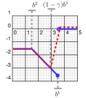
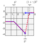
(a)	(b)

Figure 3: Comparison of the true loss $L$ with (a) the surrogate loss $L^{\prime}_{\gamma}$; (b) the surrogate loss $L_{\gamma}$, for $\gamma=0.1$.

Theorem 8

Let $H$ be a closed, convex subset of a linear space of functions containing $0$. Denote by $h^{*}_{\gamma}$ the solution of $\min_{h\in H}\mathcal{L}_{\gamma}(h)$. If $\sup_{{\mathbf{b}}\in\mathcal{B}}b^{(1)}=M<\infty$, then

$$\mathcal{L}(h^{*}_{\gamma})-\mathcal{L}_{\gamma}(h^{*}_{\gamma})\leq\gamma M.$$

The following sets, which will be used in our proof, form a partition of $\mathcal{X}\times\mathcal{B}$

$$I_{1} =\{({\mathbf{x}},{\mathbf{b}})|h^{*}_{\gamma}({\mathbf{x}})\leq b^{(2)}\} I_{2} =\{({\mathbf{x}},{\mathbf{b}})|h^{*}_{\gamma}({\mathbf{x}})\in(b^{(2)},b^{(1)}]\}$$

$$I_{3} =\{({\mathbf{x}},{\mathbf{b}})|h^{*}_{\gamma}({\mathbf{x}})\in(b^{(1)},(1+\gamma)b^{(1)}]\} I_{4} =\{({\mathbf{x}},{\mathbf{b}})|h^{*}_{\gamma}({\mathbf{x}})>(1+\gamma)b^{(1)}\}$$

This sets represent the different regions where $L_{\gamma}$ is defined. In each region the function is affine. We will now prove a technical lemma that will help us in the proof of Theorem 8.

Lemma 9

Under the conditions of Theorem 8,

$$\operatorname*{\mathbb{E}}_{{\mathbf{x}},{\mathbf{b}}}\Big{[}h^{*}_{\gamma}({\mathbf{x}})\mathds{1}_{I_{2}}({\mathbf{x}})\Big{]}\geq\frac{1}{\gamma}\operatorname*{\mathbb{E}}_{{\mathbf{x}},{\mathbf{b}}}\Big{[}h^{*}_{\gamma}({\mathbf{x}})\mathds{1}_{I_{3}}({\mathbf{x}})\Big{]}.$$

Proof  Let $0<\lambda<1$. Since $H$ is a convex set, it follows that $\lambda h^{*}_{\gamma}\in H$; and from the definition of $h^{*}_{\gamma}$ we must have:

$$\operatorname*{\mathbb{E}}_{{\mathbf{x}},{\mathbf{b}}}\Big{[}L_{\gamma}(h^{*}_{\gamma}({\mathbf{x}}),{\mathbf{b}})\Big{]}\leq\operatorname*{\mathbb{E}}_{{\mathbf{x}},{\mathbf{b}}}\Big{[}L_{\gamma}(\lambda h^{*}_{\gamma}({\mathbf{x}}),{\mathbf{b}})\Big{]}.$$ (7)

If $h^{*}_{\gamma}({\mathbf{x}})<0$, then $L_{\gamma}(h^{*}_{\gamma}({\mathbf{x}}),{\mathbf{b}})=L_{\gamma}(\lambda h^{*}_{\gamma}({\mathbf{x}}))=-b^{(2)}$ by definition of $L_{\gamma}$. If on the other hand $h^{*}_{\gamma}({\mathbf{x}})>0$, since $\lambda h^{*}_{\gamma}({\mathbf{x}})<h^{*}_{\gamma}({\mathbf{x}})$ we must have that for $({\mathbf{x}},{\mathbf{b}})\in I_{1}\;L_{\gamma}(h^{*}_{\gamma}({\mathbf{x}}),{\mathbf{b}})=L_{\gamma}(\lambda h^{*}_{\gamma}({\mathbf{x}}),{\mathbf{b}})=-b^{(2)}$ too. Moreover, from the fact that $L_{\gamma}\leq 0$ and $L_{\gamma}(h^{*}_{\gamma}({\mathbf{x}}),{\mathbf{b}})=0$ for $({\mathbf{x}},{\mathbf{b}})\in I_{4}$ it follows that $L_{\gamma}(h^{*}_{\gamma}({\mathbf{x}}),{\mathbf{b}})\geq L_{\gamma}(\lambda h^{*}_{\gamma}({\mathbf{x}}),{\mathbf{b}})$ for $({\mathbf{x}},{\mathbf{b}})\in I_{4}$, and therefore the following inequality trivially holds:

$$\operatorname*{\mathbb{E}}_{{\mathbf{x}},{\mathbf{b}}}\Big{[}L_{\gamma}(h^{*}_{\gamma}({\mathbf{x}}),{\mathbf{b}})(\mathds{1}_{I_{1}}({\mathbf{x}})+\mathds{1}_{I_{4}}({\mathbf{x}}))\Big{]}\geq\operatorname*{\mathbb{E}}_{{\mathbf{x}},{\mathbf{b}}}\Big{[}L_{\gamma}(\lambda h^{*}_{\gamma}({\mathbf{x}}),{\mathbf{b}})(\mathds{1}_{I_{1}}({\mathbf{x}})+\mathds{1}_{I_{4}}({\mathbf{x}}))\Big{]}.$$ (8)

Subtracting (8) from (7) we obtain

$$\operatorname*{\mathbb{E}}_{{\mathbf{x}},{\mathbf{b}}}\Big{[}L_{\gamma}(h^{*}_{\gamma}({\mathbf{x}}),{\mathbf{b}})(\mathds{1}_{I_{2}}({\mathbf{x}})+\mathds{1}_{I_{3}}({\mathbf{x}}))\Big{]}\leq\operatorname*{\mathbb{E}}_{{\mathbf{x}},{\mathbf{b}}}\Big{[}L_{\gamma}(\lambda h^{*}_{\gamma}({\mathbf{x}}),{\mathbf{b}})(\mathds{1}_{I_{2}}({\mathbf{x}})+\mathds{1}_{I_{3}}({\mathbf{x}}))\Big{]}.$$

By rearranging terms we can see this inequality is equivalent to

$$\operatorname*{\mathbb{E}}_{{\mathbf{x}},{\mathbf{b}}}\Big{[}(L_{\gamma}(\lambda h^{*}_{\gamma}({\mathbf{x}}),{\mathbf{b}})-L_{\gamma}(h^{*}_{\gamma}({\mathbf{x}}),{\mathbf{b}}))\mathds{1}_{I_{2}}({\mathbf{x}})\Big{]}\geq\operatorname*{\mathbb{E}}_{{\mathbf{x}},{\mathbf{b}}}\Big{[}(L_{\gamma}(h^{*}_{\gamma}({\mathbf{x}}),{\mathbf{b}})-L_{\gamma}(\lambda h^{*}_{\gamma}({\mathbf{x}}),{\mathbf{b}}))\mathds{1}_{I_{3}}({\mathbf{x}})\Big{]}$$ (9)

Notice that if $({\mathbf{x}},{\mathbf{b}})\in I_{2}$, then $L_{\gamma}(h^{*}_{\gamma}({\mathbf{x}}),{\mathbf{b}})=-h^{*}_{\gamma}({\mathbf{x}})$. If $\lambda h^{*}_{\gamma}({\mathbf{x}})>b^{(2)}$ too then $L_{\gamma}(\lambda h^{*}_{\gamma}({\mathbf{x}}),{\mathbf{b}})=-\lambda h^{*}_{\gamma}({\mathbf{x}})$. On the other hand if $\lambda h^{*}_{\gamma}({\mathbf{x}})\leq b^{(2)}$ then $L_{\gamma}(\lambda h^{*}_{\gamma}({\mathbf{x}}),{\mathbf{b}})=-b^{(2)}\leq-\lambda h^{*}_{\gamma}({\mathbf{x}})$. Thus

$$\operatorname*{\mathbb{E}}(L_{\gamma}(\lambda h^{*}_{\gamma}({\mathbf{x}}),{\mathbf{b}})-L_{\gamma}(h^{*}_{\gamma}({\mathbf{x}}),{\mathbf{b}}))\mathds{1}_{I_{2}}({\mathbf{x}}))\leq(1-\lambda)\operatorname*{\mathbb{E}}(h^{*}_{\gamma}({\mathbf{x}})\mathds{1}_{I_{2}}({\mathbf{x}}))$$ (10)

This gives an upper bound for the left-hand side of inequality (9). We now seek to derive a lower bound on the right-hand side. To do that, we analyze two different cases:

1. $\lambda h^{*}_{\gamma}({\mathbf{x}})\leq b^{(1)}$;

2. $\lambda h^{*}_{\gamma}({\mathbf{x}})>b^{(1)}$.

In the first case, we know that $L_{\gamma}(h^{*}_{\gamma}({\mathbf{x}}),{\mathbf{b}})=\frac{1}{\gamma}(h^{*}_{\gamma}({\mathbf{x}})-(1+\gamma)b^{(1)})>-b^{(1)}$ (since $h^{*}_{\gamma}({\mathbf{x}})>b^{(1)}$ for $({\mathbf{x}},{\mathbf{b}})\in I_{3}$). Furthermore, if $\lambda h^{*}_{\gamma}({\mathbf{x}})\leq b^{(1)}$, then, by definition $L_{\gamma}(\lambda h^{*}_{\gamma}({\mathbf{x}}),{\mathbf{b}})=\min(-b^{(2)},-\lambda h^{*}_{\gamma}({\mathbf{x}}))\leq-\lambda h^{*}_{\gamma}({\mathbf{x}})$. Thus, we must have:

$$L_{\gamma}(h^{*}_{\gamma}({\mathbf{x}}),{\mathbf{b}})-L_{\gamma}(\lambda h^{*}_{\gamma}({\mathbf{x}}),{\mathbf{b}})>\lambda h^{*}_{\gamma}({\mathbf{x}})-b^{(1)}>(\lambda-1)b^{(1)}\geq(\lambda-1)M,$$ (11)

where we used the fact that $h^{*}_{\gamma}({\mathbf{x}})>b^{(1)}$ for the second inequality and the last inequality holds since $\lambda-1<0$.

We analyze the second case now. If $\lambda h^{*}_{\gamma}({\mathbf{x}})>b^{(1)}$, then for $({\mathbf{x}},{\mathbf{b}})\in I_{3}$ we have $L_{\gamma}(h^{*}_{\gamma}({\mathbf{x}}),{\mathbf{b}})-L_{\gamma}(\lambda h^{*}_{\gamma}({\mathbf{x}}),{\mathbf{b}})=\frac{1}{\gamma}(1-\lambda)h^{*}_{\gamma}({\mathbf{x}})$. Thus, letting $\Delta({\mathbf{x}},{\mathbf{b}})=L_{\gamma}(h^{*}_{\gamma}({\mathbf{x}}),{\mathbf{b}})-L_{\gamma}(\lambda h^{*}_{\gamma}({\mathbf{x}}),{\mathbf{b}})$, we can lower bound the right-hand side of (9) as:

$$\operatorname*{\mathbb{E}}_{{\mathbf{x}},{\mathbf{b}}}\Big{[}\Delta({\mathbf{x}},{\mathbf{b}})\mathds{1}_{I_{3}}({\mathbf{x}})\Big{]} =\operatorname*{\mathbb{E}}_{{\mathbf{x}},{\mathbf{b}}}\Big{[}\Delta({\mathbf{x}},{\mathbf{b}})\mathds{1}_{I_{3}}({\mathbf{x}})\mathds{1}_{\{\lambda h^{*}_{\gamma}({\mathbf{x}})>b^{(1)}\}}\Big{]}+\operatorname*{\mathbb{E}}_{{\mathbf{x}},{\mathbf{b}}}\Big{[}\Delta({\mathbf{x}},{\mathbf{b}})\mathds{1}_{I_{3}}({\mathbf{x}})\mathds{1}_{\{\lambda h^{*}_{\gamma}({\mathbf{x}})\leq b^{(1)}\}}\Big{]}$$

$$\geq\frac{1-\lambda}{\gamma}\operatorname*{\mathbb{E}}_{{\mathbf{x}},{\mathbf{b}}}\Big{[}h^{*}_{\gamma}({\mathbf{x}})\mathds{1}_{I_{3}}({\mathbf{x}})\mathds{1}_{\{\lambda h^{*}_{\gamma}({\mathbf{x}})>b^{(1)}\}}\Big{]}+(\lambda-1)M\operatorname*{\mathbb{P}}\Big{[}h^{*}_{\gamma}({\mathbf{x}})>b^{(1)}\geq\lambda h^{*}_{\gamma}({\mathbf{x}})\Big{]},$$ (12)

where we have used (11) to bound the second summand. Combining inequalities (9), (10) and (12) and dividing by $(1-\lambda)$ we obtain the bound

$$\operatorname*{\mathbb{E}}_{{\mathbf{x}},{\mathbf{b}}}\Big{[}h^{*}_{\gamma}({\mathbf{x}})\mathds{1}_{I_{2}}({\mathbf{x}})\Big{]}\geq\frac{1}{\gamma}\operatorname*{\mathbb{E}}_{{\mathbf{x}},{\mathbf{b}}}\Big{[}h^{*}_{\gamma}({\mathbf{x}})\mathds{1}_{I_{3}}({\mathbf{x}})\mathds{1}_{\{\lambda h^{*}_{\gamma}({\mathbf{x}})>b^{(1)}\}}\Big{]}-M\operatorname*{\mathbb{P}}\Big{[}h^{*}_{\gamma}({\mathbf{x}})>b^{(1)}\geq\lambda h^{*}_{\gamma}({\mathbf{x}})\Big{]}.$$

Finally, taking the limit $\lambda\rightarrow 1$, we obtain

$$\operatorname*{\mathbb{E}}_{{\mathbf{x}},{\mathbf{b}}}\Big{[}h^{*}_{\gamma}({\mathbf{x}})\mathds{1}_{I_{2}}({\mathbf{x}})\Big{]}\geq\frac{1}{\gamma}\operatorname*{\mathbb{E}}_{{\mathbf{x}},{\mathbf{b}}}\Big{[}h^{*}_{\gamma}({\mathbf{x}})\mathds{1}_{I_{3}}({\mathbf{x}})\Big{]}.$$

Taking the limit inside the expectation is justified by the bounded convergence theorem and $\operatorname*{\mathbb{P}}[h^{*}_{\gamma}({\mathbf{x}})>b^{(1)}\geq\lambda h^{*}_{\gamma}({\mathbf{x}})]\rightarrow 0$ holds by the continuity of probability measures.  

Proof [Of Theorem 8]. We can express the difference as

$$\operatorname*{\mathbb{E}}_{{\mathbf{x}},{\mathbf{b}}}\Big{[}L(h^{*}_{\gamma}({\mathbf{x}}),{\mathbf{b}})-L_{\gamma}(h^{*}_{\gamma}({\mathbf{x}}),{\mathbf{b}})\Big{]} =\sum_{k=1}^{4}\operatorname*{\mathbb{E}}_{{\mathbf{x}},{\mathbf{b}}}\Big{[}(L(h^{*}_{\gamma}({\mathbf{x}}),{\mathbf{b}})-L_{\gamma}(h^{*}_{\gamma}({\mathbf{x}}),{\mathbf{b}}))\mathds{1}_{I_{k}}({\mathbf{x}})\Big{]}$$

$$=\operatorname*{\mathbb{E}}_{{\mathbf{x}},{\mathbf{b}}}\Big{[}(L(h^{*}_{\gamma}({\mathbf{x}}),{\mathbf{b}})-L_{\gamma}(h^{*}_{\gamma}({\mathbf{x}}),{\mathbf{b}}))\mathds{1}_{I_{3}}({\mathbf{x}})\Big{]}$$

$$=\operatorname*{\mathbb{E}}_{{\mathbf{x}},{\mathbf{b}}}\Big{[}\frac{1}{\gamma}((1+\gamma)b^{(1)}-h^{*}_{\gamma}({\mathbf{x}}))\mathds{1}_{I_{3}}({\mathbf{x}}))\Big{]}.$$ (13)

Furthermore, for $({\mathbf{x}},{\mathbf{b}})\in I_{3}$, we know that $b^{(1)}<h^{*}_{\gamma}({\mathbf{x}})$. Thus, we can bound (13) by $\operatorname*{\mathbb{E}}_{{\mathbf{x}},{\mathbf{b}}}[h^{*}_{\gamma}({\mathbf{x}})\mathds{1}_{I_{3}}({\mathbf{x}})]$, which, by Lemma 9, is less than $\gamma\operatorname*{\mathbb{E}}_{{\mathbf{x}},{\mathbf{b}}}\Big{[}h^{*}_{\gamma}({\mathbf{x}})\mathds{1}_{I_{2}}({\mathbf{x}})\big{]}$. We thus have:

$$\operatorname*{\mathbb{E}}_{{\mathbf{x}},{\mathbf{b}}}\Big{[}L(h^{*}_{\gamma}({\mathbf{x}}),{\mathbf{b}})\Big{]}-\operatorname*{\mathbb{E}}_{{\mathbf{x}},{\mathbf{b}}}\Big{[}L_{\gamma}(h^{*}_{\gamma}({\mathbf{x}}),{\mathbf{b}})\Big{]}\\ \leq\gamma\operatorname*{\mathbb{E}}_{{\mathbf{x}},{\mathbf{b}}}\Big{[}h^{*}_{\gamma}({\mathbf{x}})\mathds{1}_{I_{2}}({\mathbf{x}})\Big{]}\leq\gamma\operatorname*{\mathbb{E}}_{{\mathbf{x}},{\mathbf{b}}}\Big{[}b^{(1)}\mathds{1}_{I_{2}}({\mathbf{x}})\Big{]}\leq\gamma M,$$

since $h^{*}_{\gamma}({\mathbf{x}})\leq b^{(1)}$ for $({\mathbf{x}},{\mathbf{b}})\in I_{2}$.  
Notice that, since $L\geq L_{\gamma}$ for all $\gamma\geq 0$, it follows easily from the proposition that $\mathcal{L}_{\gamma}(h^{*}_{\gamma})\rightarrow\mathcal{L}(h^{*})$. Indeed, if $h^{*}$ is the best hypothesis in class for the real loss, then the following inequalities are straightforward:

$$0\leq\mathcal{L}_{\gamma}(h^{*})-\mathcal{L}_{\gamma}(h^{*}_{\gamma}) \leq\mathcal{L}(h^{*})-\mathcal{L}_{\gamma}(h^{*}_{\gamma})$$

$$\leq\mathcal{L}(h^{*}_{\gamma})-\mathcal{L}_{\gamma}(h^{*}_{\gamma})\leq\gamma M$$

The $1/\gamma$-Lipschitzness of $L_{\gamma}$ can be used to prove the following generalization bound.

Theorem 10

Fix $\gamma\in(0,1]$ and let $S$ denotes a sample of size $m$. Then, for any $\delta>0$, with probability at least $1-\delta$ over the choice of the sample $S$, for all $h\in H$, the following holds:

$$\mathcal{L}_{\gamma}(h)\leq\widehat{\mathcal{L}}_{\gamma}(h)+\frac{2}{\gamma}\mathfrak{R}_{m}(H)+M\sqrt{\frac{\log\frac{1}{\delta}}{2m}}.$$ (14)

Proof  Let $\mathcal{L}_{\gamma,H}$ denote the family of functions $\{({\mathbf{x}},{\mathbf{b}})\to L_{\gamma}(h({\mathbf{x}}),b)\colon h\in H\}$. The loss function $L_{\gamma}$ is $\frac{1}{\gamma}$-Lipschitz since the slope of the lines defining it is at most $\frac{1}{\gamma}$. Thus, using the contraction lemma (Lemma 18) as in the proof of Proposition 1 gives $\mathfrak{R}_{m}(\mathcal{L}_{\gamma,H})\leq\frac{1}{\gamma}\mathfrak{R}_{m}(H)$. The application of a standard Rademacher complexity bound to the family of functions $\mathcal{L}_{\gamma,H}$ then shows that for any $\delta>0$, with probability at least $1-\delta$, for any $h\in H$, the following holds:

$$\mathcal{L}_{\gamma}(h)\leq\widehat{\mathcal{L}}_{\gamma}(h)+\frac{2}{\gamma}\mathfrak{R}_{m}(H)+M\sqrt{\frac{\log\frac{1}{\delta}}{2m}}.$$

 

We conclude this section by presenting a stronger form of consistency result. We will show that we can lower bound the generalization error of the best hypothesis in class $\mathcal{L}^{*}:=\mathcal{L}(h^{*})$ in terms of that of the empirical minimizer of $L_{\gamma}$, $\widehat{h}_{\gamma}:=\operatorname*{\rm argmin}_{h\in H}\widehat{\mathcal{L}}_{\gamma}(h)$.

Theorem 11

Let $M=\sup_{b\in\mathcal{B}}b^{(1)}$ and let $H$ be a hypothesis set with pseudo-dimension $d=\text{Pdim}(H).$ Then for any $\delta>0$ and a fixed value of $\gamma>0$, with probability at least $1-\delta$ over the choice of a sample $S$ of size $m$, the following inequality holds:

$$\mathcal{L}(\widehat{h}_{\gamma})\leq\mathcal{L}^{*}+\frac{2\gamma+2}{\gamma}\mathfrak{R}_{m}(H)+\gamma M+2M\sqrt{\frac{2d\log\frac{\epsilon m}{d}}{m}}+2M\sqrt{\frac{\log\frac{2}{\delta}}{2m}}.$$

Proof  By Theorem 3, with probability at least $1-\delta/2$, the following holds:

$$\mathcal{L}(\widehat{h}_{\gamma})\leq\widehat{\mathcal{L}}_{S}(\widehat{h}_{\gamma})+2\mathfrak{R}_{m}(H)+2M\sqrt{\frac{2d\log\frac{\epsilon m}{d}}{m}}+M\sqrt{\frac{\log\frac{2}{\delta}}{2m}}.$$ (15)

Furthermore, applying Lemma 9 with the empirical distribution induced by the sample, we can bound $\widehat{\mathcal{L}}_{S}(\widehat{h}_{\gamma})$ by $\widehat{\mathcal{L}}_{\gamma}(\widehat{h}_{\gamma})+\gamma M$. The first term of the previous expression is less than $\widehat{\mathcal{L}}_{\gamma}(h^{*}_{\gamma})$ by definition of $\widehat{h}_{\gamma}$. Finally, the same analysis as the one used in the proof of Theorem 10 shows that with probability $1-\delta/2$,

$$\widehat{\mathcal{L}}_{\gamma}(h^{*}_{\gamma})\leq\mathcal{L}_{\gamma}(h_{\gamma}^{*})+\frac{2}{\gamma}\mathfrak{R}_{m}(H)+M\sqrt{\frac{\log\frac{2}{\delta}}{2m}}.$$

Again, by definition of $h^{*}_{\gamma}$ and using the fact that $L$ is an upper bound on $L_{\gamma}$, we can write $\mathcal{L}_{\gamma}(h^{*}_{\gamma})\leq\mathcal{L}_{\gamma}(h^{*})\leq\mathcal{L}(h^{*})$. Thus,

$$\widehat{\mathcal{L}}_{S}(\widehat{h}_{\gamma})\leq\mathcal{L}(h^{*})+\frac{1}{\gamma}\mathfrak{R}_{m}(H)+M\sqrt{\frac{\log\frac{2}{\delta}}{2m}}+\gamma M.$$

Combining this with (15) and applying the union bound yields the result.  
This bound can be extended to hold uniformly over all $\gamma$ at the price of a term in $O\Big{(}\frac{\sqrt{\log\log_{2}\frac{1}{\gamma}}}{\sqrt{m}}\Big{)}$. Thus, for appropriate choices of $\gamma$ and $m$ (for instance $\gamma\gg 1/m^{1/4}$) it would guarantee the convergence of $\mathcal{L}(\widehat{h}_{\gamma})$ to $\mathcal{L}^{*}$, a stronger form of consistency.

These results are reminiscent of the standard margin bounds with $\gamma$ playing the role of a margin. The situation here is however somewhat different. Our learning bounds suggest, for a fixed $\gamma\in(0,1]$, to seek a hypothesis $h$ minimizing the empirical loss $\widehat{\mathcal{L}}_{\gamma}(h)$ while controlling a complexity term upper bounding $\mathfrak{R}_{m}(H)$, which in the case of a family of linear hypotheses could be $\|h\|_{K}^{2}$ for some PSD kernel $K$. Since the bound can hold uniformly for all $\gamma$, we can use it to select $\gamma$ out of a finite set of possible grid search values. Alternatively, $\gamma$ can be set via cross-validation.

4 Algorithms

In this section we present algorithms for solving the optimization problem for selecting the reserve price. We start with the no-feature case and then treat the general case.

4.1 No feature case

We present a general algorithm to optimize sums of functions similar to $L_{\gamma}$ or $L$ in the one-dimensional case.

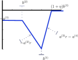
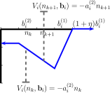
(a)	(b)

Figure 4: (a) Prototypical $v$-function. (b) Illustration of the fact that the definition of $V_{i}(r,{\mathbf{b}}_{i})$ does not change on an interval $[n_{k},n_{k+1}]$.

Definition 12

We will say that function $V\colon\mathbb{R}\times\mathcal{B}\to\mathbb{R}$ is a $v$-function if it admits the following form:

$$V(r,{\mathbf{b}})=-a^{(1)}\mathds{1}_{r\leq b^{(2)}}-a^{(2)}r\mathds{1}_{b^{(2)}<r\leq b^{(1)}}+\\ (a^{(3)}r-a^{(4)})\mathds{1}_{b^{(1)}<r<(1+\eta)b^{(1)}},$$

with $a^{(1)}>0$ and $\eta>0$ constants and $a^{(1)},a^{(2)},a^{(3)},a^{(4)}$ defined by $a^{(1)}=\eta a^{(3)}b^{(2)}$, $a^{(2)}=\eta a^{(3)}$, and $a^{(4)}=a^{(3)}(1+\eta)b^{(1)}$.

Figure 4(a) illustrates this family of loss functions. A $v$-function is a generalization of $L_{\gamma}$ and $L$. Indeed, any $v$-function $V$ satisfies $V(r,{\mathbf{b}})\leq 0$ and attains its minimum at $b^{(1)}$. Finally, as can be seen straightforwardly from Figure 3, $L_{\gamma}$ is a $v$-function for any $\gamma\geq 0$. We consider the following general problem of minimizing a sum of $v$-functions:

$$\min_{r\geq 0}\ F(r):=\sum_{i=1}^{m}V_{i}(r,{\mathbf{b}}_{i}).$$ (16)

Observe that this is not a trivial problem since, for any fixed ${\mathbf{b}}_{i}$, $V_{i}(\cdot,{\mathbf{b}}_{i})$ is non-convex and that, in general, a sum of $m$ such functions may admit many local minima. The following proposition shows that the minimum is attained at one of the highest bids, which matches the intuition.

Proposition 13

Problem (16) admits a solution $r^{*}$ that satisfies $r^{*}=b^{(1)}_{i}$ for some $i\in[1,m]$.

In order to proof this proposition a pair of lemmas are required.

Definition 14

For any $r\in\mathbb{R}$, define the following subset of $\mathbb{R}$:

$$\Omega(r)=\{\epsilon|r<b^{(1)}_{i}\leftrightarrow r+\epsilon\leq b^{(1)}_{i}\ \forall i\}$$

We will drop the dependency on $r$ when this value is understood from context.

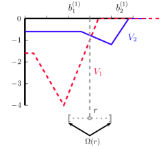
Figure 5: Illustration of the region $\Omega(r)$. The functions $V_{i}$ are monotonic and concave when restricted to this region.

Lemma 15

Let $r\neq b^{(1)}_{i}$ for all $i$. If $\epsilon>0$ is such that $[-\epsilon,\epsilon]\subset\Omega(r)$ then $F(r+\epsilon)<F(r)$ or $F(r-\epsilon)\leq F(r)$.

Proof  Let $v_{i}=V_{i}(r,{\mathbf{b}}_{i})$ and $v_{i}(\epsilon)=V_{i}(r+\epsilon,{\mathbf{b}}_{i})$. For $\epsilon\in\Omega(r)$ define the sets $D(\epsilon)=\{i~{}|~{}v_{i}(\epsilon)\leq v_{i}\}$ and $I(\epsilon)=\{i~{}|~{}v_{i}(\epsilon)>v_{i}\}$. If

$$\sum_{i\in D(\epsilon)}v_{i}+\sum_{i\in I(\epsilon)}v_{i}>\sum_{i\in D(\epsilon)}v_{i}(\epsilon)+\sum_{i\in I(\epsilon)}v_{i}(\epsilon),$$

then, by definition, we have $F(r)>F(r+\epsilon)$ and the result is proven. If this inequality is not satisfied, then, by grouping indices in $D(\epsilon)$ and $I(\epsilon)$ we must have

$$\sum_{i\in D(\epsilon)}v_{i}-v_{i}(\epsilon)~{}\leq~{}\sum_{i\in I(\epsilon)}v_{i}(\epsilon)-v_{i}$$ (17)

Notice that $v_{i}(\epsilon)\leq v_{i}$ if and only if $v_{i}(-\epsilon)\geq v_{i}$. Indeed, the function $V_{i}(r+\eta,{\mathbf{b}}_{i})$ is monotone for $\eta\in[-\epsilon,\epsilon]$ as long as $[-\epsilon,\epsilon]\subset\Omega$ which is true by the choice of $\epsilon$. This fact can easily be seen in Figure 5. Hence $D(\epsilon)=I(-\epsilon)$, similarly $I(\epsilon)=D(-\epsilon)$ Furthermore, because $V_{i}(r+\eta,{\mathbf{b}}_{i})$ is also concave for $\eta\in[-\epsilon,\epsilon]$. We must have

$$\frac{1}{2}(v_{i}(-\epsilon)+v_{i}(\epsilon))\leq v_{i}.$$ (18)

Using (18), the following inequalities are easily derived:

$$v_{i}(-\epsilon)-v_{i} \leq v_{i}-v_{i}(\epsilon) \qquad\text{for }i\in D(\epsilon)$$ (19)

$$v_{i}(\epsilon)-v_{i} \leq v_{i}-v_{i}(-\epsilon) \qquad\text{for }i\in I(\epsilon).$$ (20)

Combining inequalities (19), (17) and (20) we obtain

$$\sum_{i\in D(\epsilon)}v_{i}(-\epsilon)-v_{i} \leq\sum_{i\in I(\epsilon)}v_{i}-v_{i}(-\epsilon)$$

$$\Rightarrow\quad\sum_{i\in I(-\epsilon)}v_{i}(-\epsilon)-v_{i} \leq\sum_{i\in D(-\epsilon)}v_{i}-v_{i}(-\epsilon).$$

By rearranging back the terms in the inequality we can easily see that $F(r-\epsilon)\leq F(r)$.  

Lemma 16

Under the conditions of Lemma 15, if $F(r+\epsilon)\leq F(r)$ then $F(r+\lambda\epsilon)\leq F(r)$ for every $\lambda$ that satisfies $\lambda\epsilon\in\Omega$ if and only if $\epsilon\in\Omega$.

Proof  The proof follows the same ideas as those used in the previous lemma. By assumption, we can write

$$\sum_{D(\epsilon)}v_{i}-v_{i}(\epsilon)\geq\sum_{i\in I(\epsilon)}v_{i}(\epsilon)-v_{i}.$$ (21)

It is also clear that $I(\epsilon)=I(\lambda\epsilon)$ and $D(\epsilon)=D(\lambda\epsilon)$. Furthermore, the same concavity argument of Lemma 15 also yields:

$$v_{i}(\epsilon)\geq\frac{\lambda-1}{\lambda}v_{i}+\frac{1}{\lambda}v_{i}(\lambda\epsilon),$$

which can be rewritten as

$$\frac{1}{\lambda}(v_{i}-v_{i}(\lambda\epsilon))\geq v_{i}-v_{i}(\epsilon).$$ (22)

Applying inequality (22) in (21) we obtain

$$\frac{1}{\lambda}\sum_{D(\lambda\epsilon)}v_{i}-v_{i}(\lambda\epsilon)\geq\frac{1}{\lambda}\sum_{I(\lambda\epsilon)}v_{i}(\lambda\epsilon)-v_{i}.$$

Since $\lambda>0$, we can multiply the inequality by $\lambda$ to derive an inequality similar to (21) which implies that $F(r+\lambda\epsilon)\leq F(r)$.  

Proof  (Of Proposition 13) Let $r\neq b^{(1)}_{i}$ for every $i$. By Lemma 15, we can choose $\epsilon\neq 0$ small enough with $F(r+\epsilon)\leq F(r)$. Furthermore if $\lambda=\min_{i}\frac{|b^{(1)}_{i}-r|}{|\epsilon|}$ then $\lambda$ satisfies the hypotheses of Lemma 16. Hence, $F(r)\geq F(r+\lambda\epsilon)=F(b_{i^{*}})$, where $i^{*}$ is the minimizer of $\frac{|b^{(1)}_{i}-r|}{|\epsilon|}$.  

Problem (16) can thus be reduced to examining the value of the function for the $m$ arguments $b^{(1)}_{i}$, $i\in[1,m]$. This yields a straightforward method for solving the optimization which consists of computing $F(b^{(1)}_{i})$ for all $i$ and taking the minimum. But, since the computation of each $F(b^{(1)}_{i})$ takes $O(m)$, the overall computational cost is in $O(m^{2})$, which can be prohibitive for even moderately large values of $m$.

Instead, we present a combinatorial algorithm to solve the optimization problem (16) in $O(m\log m)$. Let $\mathcal{N}=\bigcup_{i}\{b^{(1)}_{i},b^{(2)}_{i},(1+\eta)b^{(1)}_{i}\}$ denote the set of all boundary points associated with the functions $V(\cdot,{\mathbf{b}}_{i})$. The algorithm proceeds as follows: first, sort the set $\mathcal{N}$ to obtain the ordered sequence $(n_{1},\ldots,n_{3m})$, which can be achieved in $O(m\log m)$ using a comparison-based sorting algorithm. Next, evaluate $F(n_{1})$ and compute $F(n_{k+1})$ from $F(n_{k})$ for all $k$.

The main idea of the algorithm is the following: since the definition of $V(\cdot,b_{i})$ can only change at boundary points (see also Figure 4(b)), computing $F(n_{k+1})$ from $F(n_{k})$ can be achieved in constant time. Indeed, since between $n_{k}$ and $n_{k+1}$ there are only two boundary points, we can compute $V(n_{k+1},{\mathbf{b}}_{i})$ from $V(n_{k},{\mathbf{b}}_{i})$ by calculating $V$ for only two values of ${\mathbf{b}}_{i}$, which can be done in constant time. We now give a more detailed description and proof of correctness for the algorithm.

Proposition 17

There exists an algorithm to solve optimization problem (16) in $O(m\log m)$.

Proof  The pseudo-code for the desired algorithm is presented in Algorithm 1. Where $a_{i}^{(1)},...,a_{i}^{(4)}$ denote the parameters defining the functions $V_{i}(r,{\mathbf{b}}_{i})$.

Algorithm 1 Sorting

  $\mathcal{N}:=\bigcup_{i=1}^{m}\{b_{i}^{(1)},b_{i}^{(2)},(1+\eta)b_{i}^{(1)}\}$;

  ($n_{1},...,n_{3m})={\bf Sort}(\mathcal{N})$;

  Set $\mathbf{c}_{i}:=(c_{i}^{(1)},c_{i}^{(2)},c_{i}^{(3)},c_{i}^{(4)})=0$ for $i=1,...,3m$;

  Set $c_{1}^{(1)}=-\sum_{i=1}^{m}a_{i}^{(1)}$;

  for $j=2,...,3m$ do

     Set ${\mathbf{c}}_{j}={\mathbf{c}}_{j-1}$;

     if $n_{j-1}=b^{(2)}_{i}$ for some $i$ then

         $c_{j}^{(1)}=c_{j}^{(1)}+a_{i}^{(1)}$;

         $c_{j}^{(2)}=c_{j}^{(2)}-a_{i}^{(2)}$;

     else if $n_{j-1}=b^{(1)}_{i}$ for some $i$ then

         $c_{j}^{(2)}=c_{j}^{(2)}+a_{i}^{(2)}$;

         $c_{j}^{(3)}=c_{j}^{(3)}+a_{i}^{(3)}$;

         $c_{j}^{(4)}=c_{j}^{(4)}-a_{i}^{(4)}$;

     else

         $c_{j}^{(3)}=c_{j}^{(3)}-a_{i}^{(3)}$;

         $c_{j}^{(4)}=c_{j}^{(4)}+a_{i}^{(4)}$;

     end if

  end for

We will prove that after running Algorithm 1 we can compute $F(n_{j})$ in constant time using:

$$F(n_{j})=c_{j}^{(1)}+c_{j}^{(2)}n_{j}+c_{j}^{(3)}n_{j}+c_{j}^{(4)}.$$ (23)

This holds trivially for $n_{1}$ since by definition $n_{1}\leq b^{(2)}_{i}$ for all $i$ and therefore $F(n_{1})=-\sum_{i=1}^{m}a_{i}^{(1)}$. Now, assume that (23) holds for $j$, we prove that it must also hold for $j+1$. Suppose $n_{j}=b_{i}^{2}$ for some $i$ (the cases $n_{j}=b^{(1)}_{i}$ and $n_{j}=(1+\eta)b^{(1)}_{i}$ can be handled in the same way). Then $V_{i}(n_{j},{\mathbf{b}}_{i})=-a_{i}^{(1)}$ and we can write

$$\sum_{k\neq i}V_{k}(n_{j},{\mathbf{b}}_{k})=F(n_{j})-V(n_{j},{\mathbf{b}}_{i})=(c^{(1)}_{j}+c_{j}^{(2)}n_{j}+c_{j}^{(3)}n_{j}+c_{j}^{(4)})+a_{i}^{(1)}.$$

Thus, by construction we would have:

$$c_{j+1}^{(1)}+c_{j+1}^{(2)}n_{j+1}+c_{j+1}^{(3)}n_{j+1}+c_{j+1}^{(4)} =c^{(1)}_{j}+a_{i}^{(1)}+(c_{j}^{(2)}-a_{i}^{(2)})n_{j+1}+c_{j}^{(3)}n_{j+1}+c_{j}^{(4)}$$

$$=(c^{(1)}_{j}+c_{j}^{(2)}n_{j+1}+c_{j}^{(3)}n_{j+1}+c_{j}^{(4)})+a_{i}^{(1)}-a_{i}^{(2)}n_{j+1}$$

$$=\sum_{k\neq i}V_{k}(n_{j+1},{\mathbf{b}}_{k})-a_{i}^{(2)}n_{j+1},$$

where the last equality holds since the definition of $V_{k}(r,{\mathbf{b}}_{k})$ does not change for $r\in[n_{j},n_{j+1}]$ and $k\neq i$. Finally, since $n_{j}$ was a boundary point, the definition of $V_{i}(r,{\mathbf{b}}_{i})$ must change from $-a_{i}^{(1)}$ to $-a_{i}^{(2)}r$, thus the last equation is indeed equal to $F(n_{j+1})$. A similar argument can be given if $n_{j}=b^{(1)}_{i}$ or $n_{j}=(1+\eta)b^{(1)}_{i}$.

Let us analyze the complexity of the algorithm: sorting the set $\mathcal{N}$ can be performed in $O(m\log m)$ and each iteration takes only constant time. Thus the evaluation of all points can be done in linear time. Having found all values, the minimum can also be obtained in linear time. Thus, the overall time complexity of the algorithm is $O(m\log m)$.  

The algorithm just proposed can be straightforwardly extended to solve the minimization of $F$ over a set of $r$-values bounded by $\Lambda$, that is $\{r\colon 0\leq r\leq\Lambda\}$. Indeed, we then only need to compute $F(b^{(1)}_{i})$ for $i\in[1,m]$ such that $b^{(1)}_{i}<\Lambda$ and of course also $F(\Lambda)$, thus the computational complexity in that regularized case remains $O(m\log m)$.

4.2 General case

We first consider the case of a hypothesis set $H$ of linear functions ${\mathbf{x}}\mapsto{\mathbf{w}}\cdot{\mathbf{x}}$ with bounded norm, $\|{\mathbf{w}}\|\leq\Lambda$, for some $\Lambda\geq 0$. This can be immediately generalized to the case where a positive definite kernel is used.

The results of Theorem 10 suggest seeking, for a fixed $\gamma\geq 0$, the vector ${\mathbf{w}}$ solution of the following optimization problem: $\min_{\|{\mathbf{w}}\|\leq\Lambda}\sum_{i=1}^{m}L_{\gamma}({\mathbf{w}}\cdot{\mathbf{x}}_{i},{\mathbf{b}}_{i})$. Replacing the original loss $L$ with $L_{\gamma}$ helped us remove the discontinuity of the loss. But, we still face an optimization problem based on a sum of non-convex functions. This problem can be formulated as a DC-programming (difference of convex functions programming) problem. Indeed, $L_{\gamma}$ can be decomposed as follows for all $(r,{\mathbf{b}})\in\mathcal{X}\times\mathcal{B}$: $L_{\gamma}(r,{\mathbf{b}})=u(r,{\mathbf{b}})-v(r,{\mathbf{b}})$, with the convex functions $u$ and $v$ defined by

$$u(r,{\mathbf{b}}) =-r\mathds{1}_{r<b^{(1)}}+\tfrac{r-(1+\gamma)b^{(1)}}{\gamma}\mathds{1}_{r\geq b^{(1)}}$$

$$v(r,{\mathbf{b}}) =(-r+b^{(2)})\mathds{1}_{r<b^{(2)}}+\tfrac{r-(1+\gamma)b^{(1)}}{\gamma}\mathds{1}_{r>(1+\gamma)b^{(1)}}.$$

Using the decomposition $L_{\gamma}=u-v$, our optimization problem can be formulated as follows:

$$\min_{{\mathbf{w}}\in\mathbb{R}^{N}}\ U({\mathbf{w}})-V({\mathbf{w}})\qquad\text{subject to}\ \|{\mathbf{w}}\|\leq\Lambda,$$ (24)

where $U({\mathbf{w}})=\sum_{i=1}^{m}u({\mathbf{w}}\cdot{\mathbf{x}}_{i},{\mathbf{b}}_{i})$ and $V({\mathbf{w}})=\sum_{i=1}^{m}v({\mathbf{w}}\cdot{\mathbf{x}}_{i},{\mathbf{b}}_{i})$, which shows that it can be formulated as a DC-programming problem. The global minimum of the optimization problem (24) can be found using a cutting plane method Horst and Thoai (1999), but that method only converges in the limit and does not admit known algorithmic convergence guarantees. There exists also a branch-and-bound algorithm with exponential convergence for DC-programming Horst and Thoai (1999) for finding the global minimum. Nevertheless, in Tao and An (1997), it is pointed out that this type of combinatorial algorithms fail to solve real-world DC-programs in high dimensions. In fact, our implementation of this algorithm shows that the convergence of the algorithm in practice is extremely slow for even moderately high-dimensional problems. Another attractive solution for finding the global solution of a DC-programming problem over a polyhedral convex set is the combinatorial solution of Hoang Tuy Tuy (1964). However, casting our problem as an instance of that problem requires explicitly specifying the slope and offsets for the piecewise linear function corresponding to a sum of $L_{\gamma}$ losses, which admits an exponential cost in time and space.

An alternative consists of using the DC algorithm, a primal-dual sub-differential method of Dinh Tao and Hoai An Tao and An (1998), (see also Tao and An (1997) for a good survey). This algorithm is applicable when $u$ and $v$ are proper lower semi-continuous convex functions as in our case. When $v$ is differentiable, the DC algorithm coincides with the CCCP algorithm of Yuille and Rangarajan Yuille and Rangarajan (2003), which has been used in several contexts in machine learning and analyzed by Sriperumbudur and Lanckriet (2012).

The general proof of convergence of the DC algorithm was given by Tao and An (1998). In some special cases, the DC algorithm can be used to find the global minimum of the problem as in the trust region problem Tao and An (1998), but, in general, the DC algorithm or its special case CCCP are only guaranteed to converge to a critical point Tao and An (1998); Sriperumbudur and Lanckriet (2012). Nevertheless, the number of iterations of the DC algorithm is relatively small. Its convergence has been shown to be in fact linear for DC-programming problems such as ours Yen et al. (2012). The algorithm we are proposing goes one step further than that of Tao and An (1998): we use DCA to find a local minimum but then restart our algorithm with a new seed that is guaranteed to reduce the objective function. Unfortunately, we are not in the same regime as in the trust region problem of Dinh Tao and Hoai An Tao and An (1998) where the number of local minima is linear in the size of the input. Indeed, here the number of local minima can be exponential in the number of dimensions of the feature space and it is not clear to us how the combinatorial structure of the problem could help us rule out some local minima faster and make the optimization more tractable.

In the following, we describe more in detail the solution we propose for solving the DC-programming problem (24). The functions $v$ and $V$ are not differentiable in our context but they admit a sub-gradient at all points. We will denote by $\delta V({\mathbf{w}})$ an arbitrary element of the sub-gradient $\partial V({\mathbf{w}})$, which coincides with $\nabla V({\mathbf{w}})$ at points ${\mathbf{w}}$ where $V$ is differentiable. The DC algorithm then coincides with CCCP, modulo the replacement of the gradient of $V$ by $\delta V({\mathbf{w}})$. It consists of starting with a weight vector ${\mathbf{w}}_{0}\leq\Lambda$ and of iteratively solving a sequence of convex optimization problems obtained by replacing $V$ with its linear approximation giving ${\mathbf{w}}_{t}$ as a function of ${\mathbf{w}}_{t-1}$, for $t=1,\ldots,T$: ${\mathbf{w}}_{t}\in\operatorname*{\rm argmin}_{\|{\mathbf{w}}\|\leq\Lambda}\ U({\mathbf{w}})-\delta V({\mathbf{w}}_{t-1})\cdot{\mathbf{w}}$. This problem can be rewritten in our context as the following:

$$\min_{\|{\mathbf{w}}\|\leq\Lambda,{\mathbf{s}}} \ \sum_{i=1}^{m}s_{i}-\delta V({\mathbf{w}}_{t-1})\cdot{\mathbf{w}}\mspace{10.0mu}$$ (25)

subject to $$\ (s_{i}\!\geq\!-{\mathbf{w}}\cdot{\mathbf{x}}_{i})\!\wedge\!\Big{[}\!s_{i}\!\geq\!\frac{1}{\gamma}\big{(}{\mathbf{w}}\cdot{\mathbf{x}}_{i}\!-\!(1+\gamma)b^{(1)}_{i}\big{)}\!\Big{]}.$$

The problem is equivalent to a QP (quadratic-programming) problem since the quadratic constraint can be replaced by a term of the form $\lambda\|{\mathbf{w}}\|^{2}$ in the objective and thus can be tackled using any standard QP solver. We propose an algorithm that iterates along different local minima, but with the guarantee of reducing the function at every change of local minimum. The algorithm is simple and is based on the observation that the function $L_{\gamma}$ is positive homogeneous. Indeed, for any $\eta>0$ and $(r,{\mathbf{b}})$,

$$L_{\gamma}(\eta r,\eta{\mathbf{b}}) =-\eta b^{(2)}\mathds{1}_{\eta r<\eta b^{(2)}}-\eta r\mathds{1}_{\eta b^{(2)}\leq\eta r\leq\eta b^{(1)}}+\frac{\eta r-(1+\gamma)\eta b^{(1)}}{\gamma}\mathds{1}_{\eta b^{(1)}<\eta r<\eta(1+\gamma)b^{(1)}}$$

$$=\eta L_{\gamma}(r,{\mathbf{b}}).$$

 

  DC Algorithm  

  ${\mathbf{w}}\leftarrow{\mathbf{w}}_{0}\mspace{90.0mu}\triangleright\text{initialization}$

  for $t\geq 1$ do

     ${\mathbf{w}}_{t}\leftarrow\text{\sc DCA}({\mathbf{w}})\quad\triangleright\text{{\sc DCA} algorithm}$

     ${\mathbf{w}}\leftarrow\text{\sc Optimize}(\text{objective},\text{fixed direction }{\mathbf{w}}_{t}/\|{\mathbf{w}}_{t}\|)$

  end for

 

Figure 6: Pseudocode of our DC-programming algorithm.

Minimizing the objective function of (24) in a fixed direction ${\mathbf{u}}$, $\|{\mathbf{u}}\|=1$, can be reformulated as follows: $\min_{0\leq\eta\leq\Lambda}\ \sum_{i=1}^{m}L_{\gamma}(\eta{\mathbf{u}}\cdot{\mathbf{x}}_{i},{\mathbf{b}}_{i})$. Since for ${\mathbf{u}}\cdot{\mathbf{x}}_{i}\leq 0$ the function $\eta\mapsto L_{\gamma}(\eta{\mathbf{u}}\cdot{\mathbf{x}}_{i},{\mathbf{b}}_{i})$ is constant equal to $-b^{(2)}_{i}$ the problem is equivalent to solving

$$\min_{0\leq\eta\leq\Lambda}\sum_{{\mathbf{u}}\cdot{\mathbf{x}}_{i}>0}L_{\gamma}(\eta{\mathbf{u}}\cdot{\mathbf{x}}_{i},{\mathbf{b}}_{i}).$$

Furthermore, since $L_{\gamma}$ is positive homogeneous, for all $i\in[1,m]$ with ${\mathbf{u}}\cdot{\mathbf{x}}_{i}>0$, $L_{\gamma}(\eta{\mathbf{u}}\cdot{\mathbf{x}}_{i},{\mathbf{b}}_{i})=({\mathbf{u}}\cdot{\mathbf{x}}_{i})L_{\gamma}(\eta,{\mathbf{b}}_{i}/({\mathbf{u}}\cdot{\mathbf{x}}_{i}))$. But $\eta\mapsto({\mathbf{u}}\cdot{\mathbf{x}}_{i})L_{\gamma}(\eta,{\mathbf{b}}_{i}/({\mathbf{u}}\cdot{\mathbf{x}}_{i}))$ is a $v$-function and thus the problem can efficiently optimized using the combinatorial algorithm for the no-feature case (Section 4.1). This leads to the optimization algorithm described in Figure 6. The last step of each iteration of our algorithm can be viewed as a line search and this is in fact the step that reduces the objective function the most in practice. This is because we are then precisely minimizing the objective function even though this is for some fixed direction. Since in general this line search does not find a local minimum (we are likely to decrease the objective value in other directions that are not the one in which the line search was performed) running DCA helps us find a better direction for the next iteration of the line search.

5 Experiments

In this section we report the results of several experiments done on synthetic, as well as realistic data demonstrating the benefits of our algorithm. Since the use of features for reserve price optimization is a completely novel idea, we are not aware of any baseline for comparison with our algorithm. Therefore, its performance is measured against three natural strategies that we now describe.

As mentioned before, a standard solution for solving this problem would be the use of a convex surrogate loss. For that reason, we compare against the solution of the regularized minimization of the convex surrogate loss $L_{\alpha}$ shown in Figure 1(b) parametrized by $\alpha\in[0,1]$ and defined by

$$L_{\alpha}(r,{\mathbf{b}})\!=\!\begin{cases}-r\mspace{100.0mu}\text{if }r<b^{(1)}+\alpha(b^{(2)}-b^{(1)})\\ \left(\frac{(1-\alpha)b^{(1)}+\alpha b^{(2)}}{\alpha(b^{(1)}-b^{(2)})}\right)\!(r-b^{(1)})\mspace{40.0mu}\text{otherwise}.\end{cases}$$

A second alternative consists of using ridge regression to estimate the first bid and use its prediction as the reserve price. A third algorithm consists of minimizing the loss while ignoring the feature vectors ${\mathbf{x}}_{i}$, i.e., solving the problem $\min_{r\leq\Lambda}\sum_{i=1}^{n}L(r,{\mathbf{b}}_{i})$. It is worth mentioning that this third approach is very similar to what advertisement exchanges currently use to suggest reserve prices to publishers. By using the empirical version of Equation (1), we see this algorithm is equivalent to finding the empirical distribution of bids and optimizing the expected revenue with respect to this empirical distribution as in (Ostrovsky and Schwarz, 2011) and (Cesa-Bianchi et al., 2013).

5.1 Artificial data sets

We generated $4$ different synthetic data sets with different correlation levels between features and bids. For all our experiments, the feature vectors ${\mathbf{x}}\in\mathbb{R}^{21}$ were generated in the following way: $\tilde{{\mathbf{x}}}\in\mathbb{R}^{20}$ was sampled from a standard Gaussian distribution and ${\mathbf{x}}=(\tilde{{\mathbf{x}}},1)$ was created by adding an offset feature. We now describe the bid generating process for each of the experiments as a function of the feature vector ${\mathbf{x}}$. For our first three experiments, shown in Figure 7(a)-(c), the highest bid and second highest bid were set to $\max\Big{(}\Big{|}\sum_{i=1}^{21}x_{i}\Big{|}+\epsilon_{1},\Big{|}\sum_{i=1}^{21}\frac{x_{i}}{2}+\epsilon_{2}\Big{|}\Big{)}_{+}$ and $\min\Big{(}\Big{|}\sum_{i=1}^{21}x_{i}\Big{|}+\epsilon_{1},\Big{|}\sum_{i=1}^{21}\frac{x_{i}}{2}+\epsilon_{2}\Big{|}\Big{)}_{+}$ respectively. Where $\epsilon_{i}$ is a Gaussian random variable with mean $0$. The standard deviation of the Gaussian noise was varied over the set $\{0,0.25,0.5\}$.

For our last artificial experiment we used a generative model supported on previous empirical observations (Ostrovsky and Schwarz, 2011; Lahaie and Pennock, 2007): bids were generated by sampling two values from a lognormal distribution with means ${\mathbf{x}}\cdot{\mathbf{w}}$ and $\frac{{\mathbf{x}}\cdot{\mathbf{w}}}{2}$ and standard deviation $0.5$. Where ${\mathbf{w}}$ was random vector sampled from a standard Gaussian distribution.

For all our experiments, the parameters $\Lambda,\gamma$ and $\alpha$ were tuned by using a validation set of the same number of examples as the training set. The test set consisted of $5\mathord{,}000$ examples drawn from the same distribution as the training set. Each experiment was repeated 10 times and the mean revenue of each algorithm is shown in Figure 7. The plots are normalized in such a way that the revenue obtained by setting no reserve price is equal to $0$ and the maximum possible revenue (which can be obtained by setting the reserve price equal to the highest bid) is equal to $1$. The performance of the ridge regression algorithm is not included in Figure 7(d) as it was too inferior to be comparable with the performance of the other algorithms.

By inspecting the results in Figure 7(a) we see that even in the simplest, noiseless scenario our algorithm outperforms all other techniques. It is also worth noticing that the use of ridge regression is actually worse than using no features for training. This fact is easily understood by noticing that the square loss used in regression is symmetric. Therefore, we can expect several reserve prices to be above the highest bid, which are equivalent to zero revenue auctions. Another notable feature is that as the noise level increases, the performance of feature-based algorithms decreases. This is however true of any machine learning algorithm: if the features become less relevant to the prediction task, the performance of the algorithm will suffer. However, for the convex surrogate algorithm something more critical occurs: the performance of this algorithm actually decreases as the sample size increases, which shows that in general learning with a convex surrogate is not possible. This is an empirical verification of the inconsistency result provided in Section 3.1. This lack of calibration can also seen in Figure 7(d), where in fact the performance of this algorithm approaches the use of no reserve price.

In order to better understand the reason behind the performance discrepancy between feature-based algorithms, we analyze the reserve prices offered by each algorithm. In Figure 8(a) we see that the convex surrogate algorithm tends to offer lower reserve prices. This should be intuitively clear as high reserve prices are over-penalized by the chosen convex surrogate as shown in Figure 2. On the other hand, reserve prices suggested by the regression algorithm seem to be concentrated and symmetric around their mean, therefore we can infer that about 50% of the reserve prices offered will be higher than the highest bid thereby yielding zero revenue.

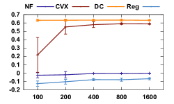
(a)	(b)
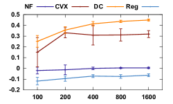
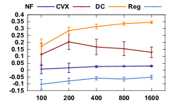
(c)	(d)

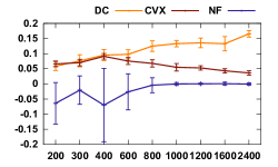
Figure 7: Plots of expected revenue against sample size for different algorithms: DC algorithm (DC), convex surrogate (CVX) and ridge regression (Reg). For (a)-(c) bids are generated with different noise standard deviation (a) 0, (b) 0.25, (c) 0.5. The bids in (d) were generated using a generative model.

5.2 Realistic data sets

Due to confidentiality and proprietary reasons, we cannot present empirical results with AdExchange data. However, we were able to secure an eBay data set consisting of collector sport cards. These cards were sold using a second price auction with reserve and the full data set can now be found in the following website:
http://cims.nyu.edu/~munoz/data. Some other sources of auction data sets are accessible (e.g. http://modelingonlineauctions.com/datasets), but no feature is available in those data sets. To the best of our knowledge, with exception of the data set used here, there is no publicly available data set for online auctions including features that could be readily used with our algorithm. The features include information about the seller such as positive feedback percent, seller rating and seller country; as well information about the card such as whether the player is in the sport’s hall of fame. The final dimension of the feature vectors is $78$. The values of these features are both continuous and categorical.

Since the highest bid is not reported by eBay, our algorithm cannot be used straightforwardly on this data set. In order to generate highest bids, we calculated the mean price of each object (each card was generally sold more than once) and set the highest bid to be the maximum between this average and the second highest bid.

On Figure 8(b) we show the revenue obtained by using our DC algorithm, a convex surrogate and the algorithm that ignores features. We also show the results obtained by using no reserve price (NR) and highest possible revenue (HB). From the whole data set 2000 examples were randomly selected for training, validation and testing. This experiment was repeated 10 times and Figure 8(b) shows the mean revenue of each algorithm and standard deviations.

(a)

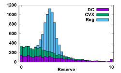
(b)

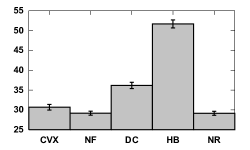
Figure 8: (a) Distribution of reserve prices for each algorithm. The algorithms were trained on 800 samples using noisy bids with standard deviation $0.5$. (b) Results of the eBay data set.

6 Conclusion

We presented a comprehensive theoretical and algorithmic analysis of the learning problem of revenue optimization in second-price auctions with reserve. The specific properties of the loss function for this problem required a new analysis and new learning guarantees. The algorithmic solutions we presented are practically applicable to revenue optimization problems for this type of auctions in most realistic settings. Our experimental results further demonstrate their effectiveness. Much of the analysis and algorithms presented, in particular our study of calibration questions, can also be of interest in other learning problems.

A Contraction lemma

The following is a version of Talagrand’s contraction lemma Ledoux and Talagrand (2011). Since our definition of Rademacher complexity does not use absolute values, we give an explicit proof below.

Lemma 18

Let $H$ be a hypothesis set of functions mapping $\mathcal{X}$ to $\mathbb{R}$ and $\Psi_{1},\ldots,\Psi_{m}$, $\mu$-Lipschitz functions for some $\mu>0$. Then, for any sample $S$ of $m$ points $x_{1},\ldots,x_{m}\in\mathcal{X}$, the following inequality holds

$$\frac{1}{m}\operatorname*{\mathbb{E}}_{{\boldsymbol{\sigma}}}\left[\sup_{h\in H}\sum_{i=1}^{m}\sigma_{i}(\Psi_{i}\circ h)(x_{i})\right] \leq\frac{\mu}{m}\operatorname*{\mathbb{E}}_{{\boldsymbol{\sigma}}}\left[\sup_{h\in H}\sum_{i=1}^{m}\sigma_{i}h(x_{i})\right]$$

$$=\mu\,\widehat{\mathfrak{R}}_{S}(H).$$

Proof  The proof is similar to the case where the functions $\Psi_{i}$ are all equal. Fix a sample $S=(x_{1},\ldots,x_{m})$. Then, we can rewrite the empirical Rademacher complexity as follows:

$$\mspace{-20.0mu}\frac{1}{m}\operatorname*{\mathbb{E}}_{{\boldsymbol{\sigma}}}\Big{[}\sup_{h\in H}\sum_{i=1}^{m}\sigma_{i}(\Psi_{i}\circ h)(x_{i})\Big{]}=\mspace{10.0mu}\frac{1}{m}\operatorname*{\mathbb{E}}_{\sigma_{1},\ldots,\sigma_{m-1}}\Big{[}\operatorname*{\mathbb{E}}_{\sigma_{m}}\Big{[}\sup_{h\in H}u_{m-1}(h)+\sigma_{m}(\Psi_{m}\circ h)(x_{m})\Big{]}\Big{]}\,,$$

where $u_{m-1}(h)=\sum_{i=1}^{m-1}\sigma_{i}(\Psi_{i}\circ h)(x_{i})$. Assume that the suprema can be attained and let $h_{1},h_{2}\in H$ be the hypotheses satisfying

$$u_{m-1}(h_{1})+\Psi_{m}(h_{1}(x_{m}))=\sup_{h\in H}u_{m-1}(h)+\Psi_{m}(h(x_{m}))$$

$$u_{m-1}(h_{2})-\Psi_{m}(h_{2}(x_{m}))=\sup_{h\in H}u_{m-1}(h)-\Psi_{m}(h(x_{m})).$$

When the suprema are not reached, a similar argument to what follows can be given by considering instead hypotheses that are $\epsilon$-close to the suprema for any $\epsilon>0$.

By definition of expectation, since $\sigma_{m}$ uniform distributed over $\{-1,+1\}$, we can write

$$\operatorname*{\mathbb{E}}_{\sigma_{m}}\Big{[}\sup_{h\in H}u_{m-1}(h)+\sigma_{m}(\Psi_{m}\circ h)(x_{m})\Big{]} =\frac{1}{2}\sup_{h\in H}u_{m-1}(h)+(\Psi_{m}\circ h)(x_{m})+\frac{1}{2}\sup_{h\in H}u_{m-1}(h)-(\Psi_{m}\circ h)(x_{m})$$

$$=\frac{1}{2}[u_{m-1}(h_{1})+(\Psi_{m}\circ h_{1})(x_{m})]+\frac{1}{2}[u_{m-1}(h_{2})-(\Psi_{m}\circ h_{2})(x_{m})].$$

Let $s=\operatorname{sgn}(h_{1}(x_{m})-h_{2}(x_{m}))$. Then, the previous equality implies

$$\operatorname*{\mathbb{E}}_{\sigma_{m}}\Big{[}\sup_{h\in H}u_{m-1}(h)+\sigma_{m}(\Psi_{m}\circ h)(x_{m})\Big{]} =\frac{1}{2}[u_{m-1}(h_{1})+u_{m-1}(h_{2})+s\mu(h_{1}(x_{m})-h_{2}(x_{m}))]$$

$$=\frac{1}{2}[u_{m-1}(h_{1})+s\mu h_{1}(x_{m})]+\frac{1}{2}[u_{m-1}(h_{2})-s\mu h_{2}(x_{m})]$$

$$\leq\frac{1}{2}\sup_{h\in H}[u_{m-1}(h)+s\mu h(x_{m})]+\frac{1}{2}\sup_{h\in H}[u_{m-1}(h)-s\mu h(x_{m})]$$

$$=\operatorname*{\mathbb{E}}_{\sigma_{m}}\Big{[}\sup_{h\in H}u_{m-1}(h)+\sigma_{m}\mu h(x_{m})\Big{]},$$

where we used the $\mu-$Lipschitzness of $\Psi_{m}$ in the first equality and the definition of expectation over $\sigma_{m}$ for the last equality. Proceeding in the same way for all other $\sigma_{i}$’s ($i\neq m$) proves the lemma.

References

- Amin et al. (2012) Kareem Amin, Michael Kearns, Peter Key, and Anton Schwaighofer. Budget optimization for sponsored search: Censored learning in MDPs. In UAI, pages 54–63, 2012.
- Balcan et al. (2008) Maria-Florina Balcan, Avrim Blum, Jason D. Hartline, and Yishay Mansour. Reducing mechanism design to algorithm design via machine learning. J. Comput. Syst. Sci., 74(8):1245–1270, 2008.
- Bartlett et al. (2006) Peter L Bartlett, Michael I Jordan, and Jon D McAuliffe. Convexity, classification, and risk bounds. Journal of the American Statistical Association, 101(473):138–156, 2006.
- Blum et al. (2004) Avrim Blum, Vijay Kumar, Atri Rudra, and Felix Wu. Online learning in online auctions. Theor. Comput. Sci., 324(2-3):137–146, 2004.
- Cesa-Bianchi et al. (2013) Nicolò Cesa-Bianchi, Claudio Gentile, and Yishay Mansour. Regret minimization for reserve prices in second-price auctions. In SODA, pages 1190–1204, 2013.
- Cui et al. (2011) Ying Cui, Ruofei Zhang, Wei Li, and Jianchang Mao. Bid landscape forecasting in online ad exchange marketplace. In KDD, pages 265–273, 2011.
- Debreu and Koopmans (1982) Gerard Debreu and Tjalling C. Koopmans. Additively decomposed quasiconvex functions. Mathematical Programming, 24, 1982.
- Devanur and Kakade (2009) Nikhil R. Devanur and Sham M. Kakade. The price of truthfulness for pay-per-click auctions. In Proceedings 10th ACM Conference on Electronic Commerce (EC-2009), Stanford, California, USA, July 6–10, 2009, pages 99–106, 2009.
- Easley and Kleinberg (2010) David A. Easley and Jon M. Kleinberg. Networks, Crowds, and Markets - Reasoning About a Highly Connected World. Cambridge University Press, 2010.
- He et al. (2013) Di He, Wei Chen, Liwei Wang, and Tie-Yan Liu. Online learning for auction mechanism in bandit setting. Decision Support Systems, 56:379–386, 2013.
- Horst and Thoai (1999) R Horst and Nguyen V Thoai. DC programming: overview. Journal of Optimization Theory and Applications, 103(1):1–43, 1999.
- Koltchinskii and Panchenko (2002) V. Koltchinskii and D. Panchenko. Empirical margin distributions and bounding the generalization error of combined classifiers. Ann. Statist., 30(1):1–50, 2002.
- Lahaie and Pennock (2007) Sébastien Lahaie and David M. Pennock. Revenue analysis of a family of ranking rules for keyword auctions. In Proceedings 8th ACM Conference on Electronic Commerce (EC-2007), San Diego, California, USA, June 11-15, 2007, pages 50–56, 2007.
- Langford et al. (2010) John Langford, Lihong Li, Yevgeniy Vorobeychik, and Jennifer Wortman. Maintaining equilibria during exploration in sponsored search auctions. Algorithmica, 58(4):990–1021, 2010.
- Ledoux and Talagrand (2011) Michel Ledoux and Michel Talagrand. Probability in Banach spaces. Classics in Mathematics. Springer-Verlag, Berlin, 2011. Isoperimetry and processes, Reprint of the 1991 edition.
- Milgrom and Weber (1982) P.R. Milgrom and R.J. Weber. A theory of auctions and competitive bidding. Econometrica: Journal of the Econometric Society, pages 1089–1122, 1982.
- Mohri et al. (2012) Mehryar Mohri, Afshin Rostamizadeh, and Ameet Talwalkar. Foundations of machine learning. MIT Press, Cambridge, MA, 2012.
- Muthukrishnan (2009) S Muthukrishnan. Ad exchanges: Research issues. Internet and network economics, pages 1–12, 2009.
- Myerson (1981) R.B. Myerson. Optimal auction design. Mathematics of operations research, 6(1):58–73, 1981.
- Nisan et al. (2007) Noam Nisan, Tim Roughgarden, Éva Tardos, and Vijay V. Vazirani, editors. Algorithmic game theory. Cambridge University Press, Cambridge, 2007.
- Ostrovsky and Schwarz (2011) Michael Ostrovsky and Michael Schwarz. Reserve prices in internet advertising auctions: a field experiment. In ACM Conference on Electronic Commerce, pages 59–60, 2011.
- Pollard (1984) David Pollard. Convergence of stochastic processes. Springer Series in Statistics. Springer-Verlag, New York, 1984.
- Riley and Samuelson (1981) J.G. Riley and W.F. Samuelson. Optimal auctions. The American Economic Review, pages 381–392, 1981.
- Sriperumbudur and Lanckriet (2012) Bharath K. Sriperumbudur and Gert R. G. Lanckriet. A proof of convergence of the concave-convex procedure using Zangwill’s theory. Neural Computation, 24(6):1391–1407, 2012.
- Tao and An (1997) Pham Dinh Tao and Le Thi Hoai An. Convex analysis approach to DC programming: theory, algorithms and applications. Acta Mathematica Vietnamica, 22(1):289–355, 1997.
- Tao and An (1998) Pham Dinh Tao and Le Thi Hoai An. A DC optimization algorithm for solving the trust-region subproblem. SIAM Journal on Optimization, 8(2):476–505, 1998.
- Tuy (1964) Hoang Tuy. Concave programming under linear constraints. Translated Soviet Mathematics, 5:1437–1440, 1964.
- Tuy (2002) Hoang Tuy. Counter-examples to some results on D.C. optimization. Technical report, Institute of Mathematics, Hanoi, Vietnam, 2002.
- Vickrey (1961) William Vickrey. Counterspeculation, auctions, and competitive sealed tenders. The Journal of finance, 16(1):8–37, 1961.
- Yen et al. (2012) Ian E.H. Yen, Nanyun Peng, Po-Wei Wang, and Shou-De Lin. On convergence rate of concave-convex procedure. In Proceedings of the NIPS 2012 Optimization Workshop, 2012.
- Yuille and Rangarajan (2003) Alan L. Yuille and Anand Rangarajan. The concave-convex procedure. Neural Computation, 15(4):915–936, 2003.
- Zhu et al. (2009) Yunzhang Zhu, Gang Wang, Junli Yang, Dakan Wang, Jun Yan, Jian Hu, and Zheng Chen. Optimizing search engine revenue in sponsored search. In Proceedings of the 32nd Annual International ACM SIGIR Conference on Research and Development in Information Retrieval, SIGIR 2009, Boston, MA, USA, July 19-23, 2009, pages 588–595, 2009.