Optimizing snake locomotion on an inclined plane

Abstract

We develop a model to study the locomotion of snakes on an inclined plane. We determine numerically which snake motions are optimal for two retrograde traveling-wave body shapes—triangular and sinusoidal waves—across a wide range of frictional parameters and incline angles. In the regime of large transverse friction coefficient, we find power-law scalings for the optimal wave amplitudes and corresponding costs of locomotion. We give an asymptotic analysis to show that the optimal snake motions are traveling-wave motions with amplitudes given by the same scaling laws found in the numerics.

I INTRODUCTION

Snake locomotion has recently drawn interest from biologists, engineers and applied mathematicians Astley and Jayne (2007); Hu et al. (2009); Maneewarn and Maneechai (2009). A lack of limbs distinguishes snake kinematics from other common forms of animal locomotions such as swimming, flying, and walking. Snakes propel themselves by a variety of gaits including slithering, sidewinding, concertina motion, and rectilinear progression Hu et al. (2009). They can move in terrestrial Gray and Lissmann (1950); Jayne (1986), aquatic Shine et al. (2003), and aerial Socha (2002) environments. Snake-like robots have shown the potential to realize similar locomotor ability, and have potential applications in confined environments like narrow crevices Erkmen et al. (2002), as well as rough terrain Yim et al. (2003). In such environments the ability to ascend an incline is fundamental, and various studies of snakes and snake-like robots have been carried out on this subject. Maneewarn and Maneechai Maneewarn and Maneechai (2009) examined the pattern of crawling gaits in narrow inclined pipes with jointed modular snake robots and found that high speeds were obtained with short-wavelength motions. Hatton and Choset Hatton and Choset (2010) focused on sidewinding gaits on inclines and presented stability conditions for snakes by comparing sidewinding to a rolling elliptical trajectory and determining the minimum aspect ratio of the sidewinding pattern to maintain stability. Marvi and Hu Marvi and Hu (2012) studied the concertina locomotion of snakes climbing on steep slopes and in vertical crevices. They found that snakes can actively orient their scales and lift portions of their bodies to vary their frictional interactions with the surroundings. Transeth et al. Transeth et al. (2008) considered the obstacle-aided locomotion of snake robots on inclined and vertical planes. Their model included both frictional forces and forces from rigid-body contacts with the obstacles, and their numerical results were consistent with their robotic studies. In this work, we focus on the slithering motion of snakes on an inclined plane by extending a recently-proposed model for motions on a horizontal plane Hu et al. (2009); Hu and Shelley (2012); Jing and Alben (2013); Alben (2013) to motions on an incline. Here the snake is a slender body whose curvature is prescribed as a function of arc length and time. For simplicity, we do not consider elasticity or viscoelasticity in the snake body. The external forces acting on the snake body are Coulomb friction with the ground, and gravity. The model has shown good agreement with biological snakes on a horizontal plane Hu et al. (2009); Hu and Shelley (2012), and previous studies have used the model to find optimally efficient snake motions. Hu and Shelley Hu and Shelley (2012) prescribed a sinusoidal traveling-wave body motion and found the optimally efficient amplitude and wavelength of the traveling wave. Jing and Alben Jing and Alben (2013) used the same model to consider the locomotion of two- and three-link snakes. They found optimal motions analytically and numerically in terms of the temporal function for the internal angles between the links. Alben Alben (2013) considered more general snake shapes and motions by optimizing the curvature as a function of arc length and time with 45 (and 180) parameters, across the space of frictional coefficients. He found that the optimal motions are two types of traveling-wave motions, retrograde and direct waves, for large and small transverse friction coefficients, respectively. In the large transverse friction coefficient regime, he showed analytically that the optimal motion is a traveling wave, and found the scaling laws for the wave amplitude and cost of locomotion with respect to the friction coefficients, both numerically and analytically.

In this paper, we confine our discussion to the regime where the transverse friction coefficient is larger than the tangential friction coefficients. This is the typical regime for biological and robotic snakes Hu and Shelley (2012); Hirose (1993). We prescribe the snake’s motion as a retrograde traveling wave with two shape profiles—triangular and sinusoidal—but with undetermined amplitudes. The triangular wave motion has analytical solutions and embodies many aspects of general traveling-wave motions. We obtain the optimal motions in terms of the amplitudes of the triangular wave in the three-parameter space of transverse frictional coefficient, tangential (forward) frictional coefficient, and the incline angle. We discuss the relative effects of these three parameters and find the upper bound on the incline angle for the snake to maintain an upward motion. We also find the power law scalings for the optimal amplitudes and corresponding costs of locomotion with respect to the three parameters. For the sinusoidal wave motion, we use a numerical method to solve for the position of the snake body from its prescribed curvature. We then obtain the optimal body shape numerically and show that it follows the same scaling laws as the triangular wave motion, providing confirmation of those results. In the last part of the paper, we analytically determine the asymptotic optima for more general snake motions in the regime of large transverse friction coefficient. We obtain the same scalings analytically as were found for the triangular and sinusoidal waves, which confirms and generalizes those results. Our study of snake locomotion can also be generalized to other locomotor systems as long as the same frictional law applies. One example is the undulatory swimming of sandfish lizards in sand Hatton et al. (2013); Ding et al. (2012).

The paper is organized as follows: Section II describes the mathematical model for snake locomotion on an inclined plane. Section III discusses the optima of the triangular wave motion, while Section IV studies the sinusoidal wave motion. The analytical asymptotic discussion is presented in Section V, and the conclusions follow in Section VI.

II MODEL

We use the same frictional snake model as Hu et al. (2009); Hu and Shelley (2012); Jing and Alben (2013); Alben (2013) to describe snake locomotion on an incline. The position of the snake is given by ${\bf X}(s,t)=(x(s,t),y(s,t))$, a function of arc length $s$ and time $t$. The unit vectors tangent and normal to the snake body are ${\hat{\bf s}}$ and ${\hat{\bf n}}$ respectively. The snake is placed on a plane inclined at angle $\alpha$ with respect to the horizontal plane. The $x$-$y$ axes are oriented with the $+x$ axis extending from origin directly up the incline and the $+y$ axis rotated 90 degrees from it and directed across the incline. Height is constant along the $y$ axis. A schematic diagram is shown in figure 1.

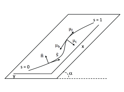
Figure 1: Schematic of the snake position on a plane inclined at angle $\alpha$. The arc length $s$ is nondimensionalized by the snake length. The tangent and normal vectors are labeled at a point. Forward, backward and transverse velocities are shown with corresponding friction coefficients $\mu_{f}$, $\mu_{b}$ and $\mu_{t}$.

The tangent angle and the curvature are denoted $\theta(s,t)$ and $\kappa(s,t)$. Given the curvature, the tangent angle and the position of the snake body can be obtained by integrating:

$$\theta(s,t) = \theta_{0}(t)+\int_{0}^{s}\kappa(s^{\prime},t)\,ds^{\prime},$$ (1)

$$x(s,t) = x_{0}(t)+\int_{0}^{s}\cos\theta(s^{\prime},t)\,ds^{\prime},$$ (2)

$$y(s,t) = y_{0}(t)+\int_{0}^{s}\sin\theta(s^{\prime},t)\,ds^{\prime}.$$ (3)

The trailing-edge position $(x_{0},y_{0})$ and the tangent angle $\theta_{0}$ are determined by the force and torque balances for the snake:

$$\int_{0}^{L}\rho\partial_{tt}xds = \int_{0}^{L}f_{x}\,ds,$$ (4)

$$\int_{0}^{L}\rho\partial_{tt}yds = \int_{0}^{L}f_{y}\,ds,$$ (5)

$$\int_{0}^{L}\rho{\bf X}^{\perp}\cdot\partial_{tt}{\bf X}\,ds = \int_{0}^{L}{\bf X}^{\perp}\cdot{\bf f}\,ds.$$ (6)

Here $\rho$ is the mass per unit length and $L$ is the length of the snake. We assume the snake is locally inextensible, and $\rho$ and $L$ are constant in time. ${\bf f}$ is the external force per unit length acting on the snake. It includes two parts: the force due to Coulomb friction with the ground Hu et al. (2009), and gravity:

$${\bf f}=\rho g\cos{\alpha}\left[-\mu_{t}\left(\widehat{\partial_{t}{\bf X}}\cdot{\hat{\bf n}}\right){\hat{\bf n}}-\left(\mu_{f}H(\widehat{\partial_{t}{\bf X}}\cdot{\hat{\bf s}})+\mu_{b}(1-H(\widehat{\partial_{t}{\bf X}}\cdot{\hat{\bf s}}))\right)\left(\widehat{\partial_{t}{\bf X}}\cdot{\hat{\bf s}}\right){\hat{\bf s}}\right]-\rho gG_{\alpha}.$$ (7)

$H(\cdot)$ is the Heaviside function, and $G_{\alpha}=(\sin\alpha,0)^{T}$ represents the component of gravity in the downhill ($-x$) direction. The hats denote normalized vectors and we define $\widehat{\partial_{t}{\bf X}}$ to be $0$ when the snake velocity is $0$. The friction coefficients are $\mu_{f},\mu_{b}$ and $\mu_{t}$ for motions in the forward $({\hat{\bf s}})$, backward $(-{\hat{\bf s}})$ and transverse $(\pm{\hat{\bf n}})$ directions. Without loss of generality we take $\mu_{f}\leq\mu_{b}$, so the forward direction has the smaller friction if it is unequal in the forward and backward directions.

We prescribe the curvature $\kappa(s,t)$ as a time-periodic function with period $T$ and nondimensionalize equations (4)-(6) by length $L$, time $T$ and mass $\rho L$. We then obtain:

$$\frac{L}{gT^{2}}\int_{0}^{1}\partial_{tt}x\,ds = \int_{0}^{1}f_{x}\,ds,$$ (8)

$$\frac{L}{gT^{2}}\int_{0}^{1}\partial_{tt}y\,ds = \int_{0}^{1}f_{y}\,ds,$$ (9)

$$\frac{L}{gT^{2}}\int_{0}^{1}{\bf X}^{\perp}\cdot\partial_{tt}{\bf X}\,ds = \int_{0}^{L}{\bf X}^{\perp}\cdot{\bf f}\,ds.$$ (10)

We neglect the snake’s inertia for simplicity, as $L/gT^{2}\ll 1$ for typical steady snake locomotion Hu et al. (2009) and set the left hand sides of (8)-(10) to zero. As discussed by Alben Alben (2013), the model still maintains a good representation of real snake motions. We then obtain the following dimensionless force and torque equations:

$$\int_{0}^{L}f_{x}ds=0,$$ (11)

$$\int_{0}^{L}f_{y}ds=0,$$ (12)

$$\int_{0}^{L}{\bf X}^{\perp}\cdot{\bf f}ds=0.$$ (13)

and the dimensionless force ${\bf f}$ becomes:

$${\bf f}=\cos{\alpha}\left[-\mu_{t}\left(\widehat{\partial_{t}{\bf X}}\cdot{\hat{\bf n}}\right){\hat{\bf n}}-\left(\mu_{f}H(\widehat{\partial_{t}{\bf X}}\cdot{\hat{\bf s}})+\mu_{b}(1-H(\widehat{\partial_{t}{\bf X}}\cdot{\hat{\bf s}}))\right)\left(\widehat{\partial_{t}{\bf X}}\cdot{\hat{\bf s}}\right){\hat{\bf s}}\right]-G_{\alpha}.$$ (14)

The frictional force tends to 0 as $\alpha$ approaches $\pi/2$. On a strictly vertically plane, frictional force is unable to balance gravity, so planar locomotion is not obtained by our model in this case (however, snakes can ascend vertical crevices in a non-planar concertina motion Marvi and Hu (2012)).

Given the curvature $\kappa(s,t)$, we solve the three nonlinear equations (11)-(13) at each time $t$ for the three unknowns $x_{0}(t),y_{0}(t)$ and $\theta_{0}(t)$. Then we obtain the snake’s position as a function of time by equations (1)-(3). We define the cost of locomotion as

$$\eta=\frac{W}{d},$$ (15)

where $d$ is the distance traveled by the snake’s center of mass over one period

$$d=\sqrt{\left(\int_{0}^{1}x(s,1)-x(s,0)\,ds\right)^{2}+\left(\int_{0}^{1}y(s,1)-y(s,0)\,ds\right)^{2}},$$ (16)

and $W$ is the work done by the snake against frictional forces and gravity over one period

$$W=\int_{0}^{1}\int_{0}^{1}-{\bf f}(s,t)\cdot\partial_{t}{\bf X}(s,t)\,ds\,dt.$$ (17)

Our objective is to find the curvature $\kappa(s,t)$ that minimizes $\eta$. We choose the initial orientation of the snake so that its center of mass travels only in the $x$ direction (up the incline) over one period of motion.

We briefly mention the case in which the snake moves down the incline, which is equivalent to setting $\alpha<0$. In this case the snake can slide down the incline with no change of shape, and the work done by gravity and friction are equal in magnitude and opposite in sign. Thus the cost of locomotion is 0 regardless of the frictional parameters. A straight body with $y(s,t)=0$ experiences purely tangential friction, and achieves the fastest speed among possible body shapes.

By contrast, when the snake ascends the incline, i.e. $\alpha\geq 0$, we will consider traveling wave motions in which net tangential friction and gravity both act in the $-x$ direction and transverse friction is necessary to balance the $x$-force equation. In the following discussions we only consider $\alpha\geq 0$, and look for nontrivial $\kappa(s,t)$ to minimize the cost of locomotion.

III TRIANGULAR WAVE BODY SHAPE

III.1 Range of $\alpha$

We start our discussion with a triangular wave body motion. It was studied on a level plane in Alben (2013), and the snake’s position, angle, velocity and work can all be obtained analytically. The motion is useful to consider because it embodies many aspects of more general traveling wave motions, while the shape dynamics are easy to understand.

The triangular wave has zero mean $y$ deflection:

$$y(s,t)=A\mathchoice{{\vbox{\hbox{$\textstyle-$ }}\kern-7.83337pt}}{{\vbox{\hbox{$\scriptstyle-$ }}\kern-5.90005pt}}{{\vbox{\hbox{$\scriptscriptstyle-$ }}\kern-4.75003pt}}{{\vbox{\hbox{$\scriptscriptstyle-$ }}\kern-4.25003pt}}\!\int\operatorname{sgn}(\sin(2\pi(s+t)))\,ds,$$ (18)

with the unit tangent and normal vectors:

$${\hat{\bf s}}=\left(\begin{array}[]{c}\sqrt{1-A^{2}}\\ A\operatorname{sgn}(\sin(2\pi(s+t)))\end{array}\right),\quad{\hat{\bf n}}=\left(\begin{array}[]{c}-A\operatorname{sgn}(\sin(2\pi(s+t)))\\ \sqrt{1-A^{2}}.\end{array}\right).$$ (19)

The force and torque balance equations are satisfied when the snake moves forward with a constant speed $U$. Then the horizontal and vertical speeds are

$$\partial_{t}x(s,t)=U,\ \partial_{t}y(s,t)=A\operatorname{sgn}(\sin(2\pi(s+t))).$$ (20)

The net $y$-force and torque for such a motion are identically zero. We determine the horizontal speed $U$ by the $x$-force balance equation:

$$\int\cos{\alpha}\left(-\mu_{t}\widehat{\partial_{t}{\bf X}}\cdot{\hat{\bf n}}n_{x}-\mu_{f}\widehat{\partial_{t}{\bf X}}\cdot{\hat{\bf s}}s_{x}\right)-\sin{\alpha}\,ds=0$$ (21)

Since $\mu_{f}\leq\mu_{b}$, and the tangential velocity is uniformly forward or backward over the whole snake body for the triangular wave, the most efficient motion is obtained when the snake moves forward. Thus $\mu_{b}$ does not appear in the frictional force in (21). Notice that the tangential frictional force and gravity both have a component in the $-x$ direction, and the transverse frictional force is the only source for a balancing force in the $+x$ direction, up the incline. Solving (21) for $U$ we obtain:

$$U=\frac{\displaystyle\left(A^{4}\left(\frac{\mu_{t}}{\mu_{f}}-1\right)^{2}+A^{2}\left(\frac{\mu_{t}}{\mu_{f}}-1\right)\right)\sqrt{1-A^{2}}-A\frac{\tan\alpha}{\mu_{f}}\sqrt{1+A^{2}\left(\frac{\mu_{t}^{2}}{\mu_{f}^{2}}-1\right)-\frac{\tan^{2}\alpha}{\mu_{f}^{2}}}}{\displaystyle\left(1+A^{2}\left(\frac{\mu_{t}}{\mu_{f}}-1\right)\right)^{2}-\frac{\tan^{2}\alpha}{\mu_{f}^{2}}}.$$ (22)

The speed of the snake is a function of $A$, $\mu_{t}$ , $\mu_{f}$ and $\alpha$. We require the speed to be real and nonnegative, and therefore the incline angle $\alpha$ must satisfy the following inequality:

$$\alpha\leq\arctan(A(\mu_{t}-\mu_{f})\sqrt{1-A^{2}}).$$ (23)

Here we use the fact that the amplitude $A\leq 1$ in the triangular wave model and $\mu_{t}>\mu_{f}$. In figure 2, we plot the upper bound of $\alpha$ according to inequality (23).

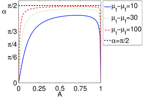
Figure 2: Lines showing the boundaries of the region on nonnegative forward velocity $U$ in the space of $A$ and $\alpha$, for different $\mu_{t}-\mu_{f}=10,30$ and $100$. On the lines, $U$ = 0, and below the lines, $U>0$. The black dashed line shows $\alpha=\pi/2$, giving a vertical incline.

For a given value of $\mu_{t}-\mu_{f}$, nonnegative speed is obtained for $\alpha$ in the region bounded by a curved line (labeled by $\mu_{t}-\mu_{f}$) and the horizontal ($A$) axis. As $\mu_{t}$ increases, larger transverse friction can be generated for the same $A$, and therefore the range of $\alpha$ increases accordingly. As $\mu_{f}$ becomes larger, the tangential motion produces a stronger downhill drag which inhibits upward motion, so the corresponding $\alpha$ range decreases. When the amplitude $A$ varies from 0 to 1, both the transverse and tangential frictional forces vary and their $x$-components have opposite sign. As a result, the range of $\alpha$ is non-monotonic with respect to $A$. The largest upper bound is obtained at $A=\sqrt{2}/2$.

III.2 Optima and other results

In the triangular wave motion, the velocity and power are both constant over time, so we can simplify the cost of locomotion as

$$\eta=\frac{W}{d}=\frac{P}{U}=\frac{\displaystyle\int_{0}^{1}-{\bf f}\cdot\partial_{t}{\bf X}ds}{U},$$ (24)

and obtain

$$\eta=\frac{\cos\alpha}{\sqrt{U^{2}+A^{2}}}\left(A^{2}(\mu_{t}-\mu_{f})\left(U-2\sqrt{1-A^{2}}-\frac{A^{2}}{U}\right)+\mu_{f}U+\frac{\mu_{t}A^{2}}{U}\right)+\sin\alpha.$$ (25)

We plug the value of $U$ (22) into (25) and minimize $\eta$ with respect to $A$. Then in the large-$\mu_{t}$ limit we obtain the optimal cost of locomotion and corresponding amplitude as:

$$\min\eta\longrightarrow(\mu_{f}\cos\alpha+\sin\alpha)\left(1+\left(\frac{2\mu_{f}}{\mu_{t}}\right)^{1/2}\right),$$ (26)

$$A\longrightarrow 2^{1/4}\mu_{t}^{-1/4}\left(\mu_{f}^{1/2}+\frac{\tan\alpha}{\mu_{f}^{1/2}}\right)^{1/2}.$$ (27)

We plot the optimal motion with $\alpha=\pi/4$, $\mu_{f}=1$ and $\mu_{t}=10$ over one period in figure 3. We manually offset the body by a constant increment in the $-y$ direction with every snapshot to clearly show the individual bodies, but we note that for the triangular wave motion, the snake’s center of mass moves purely along the $x$-axis. The peak of the snake shifts to the left in the figure, which indicates the snake moves slower than the traveling triangular wave. The snake slips transversely in the $-x$ direction to obtain a thrust force in the $+x$ direction that balances the drag forces due to tangential friction and gravity.

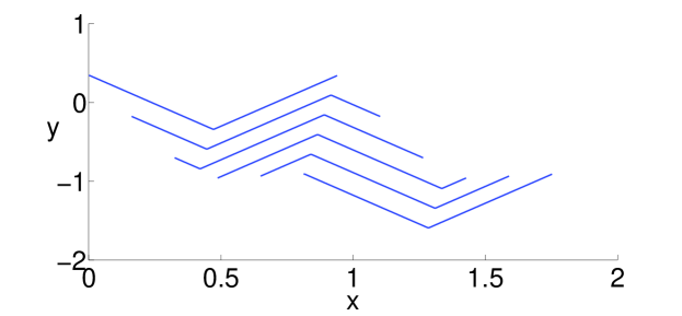
Figure 3: The optimal snake trajectory of the triangular wave body shape over one period obtained with $\alpha=\pi/4$, $\mu_{f}=1$ and $\mu_{t}=10$.

In figure 4 we plot the optimal $A$ and $\eta$ with respect to $\alpha$, $\mu_{t}$, and $\mu_{f}$. Our results extend to $\mu_{t}$ below the large-$\mu_{t}$ limit, but in this limit the results agree with (26) and (27). For each parameter set, we minimize $\eta$ over $A$ using equations (22) and (25).

$\bf{(a)}$	$\bf{(b)}$
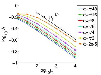
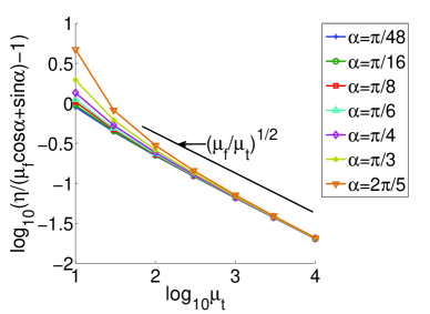
$\bf{(c)}$	$\bf{(d)}$

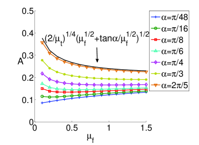
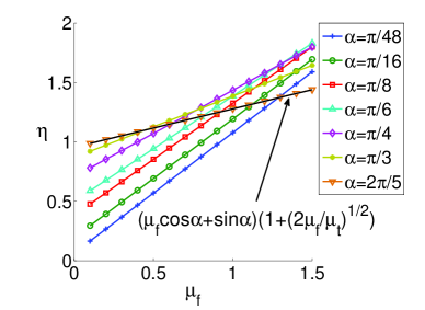
Figure 4: Scaling laws of the triangle wave optima. (a) $\log_{10}A$ vs. $\log_{10}\mu_{t}$ with various $\alpha$ and fixed $\mu_{f}=1$. The solid line indicates the scaling $\mu_{t}^{-1/4}$. (b) $\log_{10}(\eta/(\mu_{f}\cos\alpha+\sin\alpha)-1)$ vs. $\log_{10}\mu_{t}$ with various $\alpha$ and fixed $\mu_{f}=1$. The solid line shows the scaling $(\mu_{f}/\mu_{t})^{1/2}$. (c) $A$ vs. $\mu_{f}$ with various $\alpha$ and fixed $\mu_{t}=10000$. The solid line is the asymptotic solution $A=2^{1/4}\mu_{t}^{-1/4}(\mu_{f}^{1/2}+\tan\alpha/\mu_{f}^{1/2})^{1/2}$, obtained with $\alpha=2\pi/5$. (d) $\eta$ vs. $\mu_{f}$ with various $\alpha$ and fixed $\mu_{t}=10000$. The solid line shows the asymptotic optima $\eta=(\mu_{f}\cos\alpha+\sin\alpha)(1+(2\mu_{f}/\mu_{t})^{1/2})$ with $\alpha=2\pi/5$.

We plot $A$ versus $\mu_{t}$ in figure 4a with fixed $\mu_{f}=1$ and vary the parameter $\alpha$. The asymptotic scaling of $\mu_{t}^{-1/4}$ is shown with the solid line. The corresponding $\eta$ and the scaling $(\mu_{f}/\mu_{t})^{1/2}$ (solid line) are plotted in figure 4b. The optimal magnitude $A$ and cost of locomotion $\eta$ both decrease with larger $\mu_{t}$. We vary $\mu_{f}$ and $\alpha$ in figure 4c and d with fixed $\mu_{t}=10000$, and plot the optimal $A$ versus $\mu_{f}$ and $\eta$ versus $\mu_{f}$ respectively. The analytical solutions of (26) and (27) for $\alpha=2\pi/5$ are shown with solid lines in both figures, and they agree well with the numerical results at the largest $\mu_{t}$ (downward-pointing triangles). The optimal amplitude $A$ achieves its minimum at $\mu_{f}=\tan\alpha$, while the cost of locomotion $\eta$ monotonically increases with $\mu_{f}$ as $\partial_{\mu_{f}}\eta>0$. When $\alpha$ goes up, the optimal $A$ increases accordingly and its minimum over $\mu_{f}$ shifts to larger $\mu_{f}$ (figure 4c). But the cost of locomotion varies non-monotonically with $\alpha$. We can rewrite (27) as

$$\min\eta\longrightarrow\sqrt{\mu_{f}^{2}+1}\sin\left(\alpha+\arcsin\frac{\mu_{f}}{\sqrt{\mu_{f}^{2}+1}}\right)\left(1+\left(\frac{2\mu_{f}}{\mu_{t}}\right)^{1/2}\right),$$ (28)

The least efficient optimum is obtained when

$$\alpha^{*}=\frac{\pi}{2}-\arcsin\frac{\mu_{f}}{\sqrt{\mu_{f}^{2}+1}}.$$ (29)

We call $\alpha^{*}$ the critical incline angle. The optimal snake moves more efficiently when the incline is either shallower or steeper than the incline at the critical angle. The critical incline angle $\alpha^{*}$ only depends on the tangential friction coefficient and becomes smaller as $\mu_{f}$ increases. On a steeper slope, more work is done against gravity and less work against forward friction, for a given distance travelled. Thus when $\mu_{f}$ increases, efficiency can be improved by making the slope steeper (and adjusting the amplitude to achieve the optimum at the new set of parameters).

To better understand the effects of the parameters $\mu_{t},\mu_{f}$, and $\alpha$, we plot the costs of locomotion due to transverse friction alone and tangential friction alone versus $A$ in figure 5. We decompose the cost of locomotion (25) into three parts:

$$\eta=\eta_{t}+\eta_{f}+\eta_{g},$$ (30)

where

$$\eta_{t} = \frac{\cos\alpha}{\sqrt{U^{2}+A^{2}}}\left(UA^{2}\mu_{t}-2A^{2}\sqrt{1-A^{2}}\mu_{t}-\frac{A^{4}\mu_{t}}{U}+\frac{A^{2}\mu_{t}}{U}\right),$$ (31)

$$\eta_{f} = \frac{\cos\alpha}{\sqrt{U^{2}+A^{2}}}\left(U\mu_{f}(1-A^{2})+2A^{2}\sqrt{1-A^{2}}\mu_{f}+\frac{A^{4}\mu_{f}}{U}\right),$$ (32)

$$\eta_{g} = \sin\alpha$$ (33)

are the costs due to transverse friction, forward tangential friction, and gravity, respectively.

In figure 5, we vary one of the parameters $\mu_{t},\mu_{f}$, and $\alpha$ in turn and keep the other two fixed. We use solid lines for transverse friction and dashed lines for tangential friction in all panels. In general, as the amplitude $A$ becomes larger, the cost due to transverse friction decreases while the cost due to tangential friction increases. The optimal $\eta$ is obtained when the slopes of the two costs are equal in magnitude and opposite in sign. $\eta_{g}$ is independent of $A$ so it does not play a role in determining the optimal amplitude with respect to $A$.

$\bf{(a)}$	$\bf{(b)}$	$\bf{(c)}$

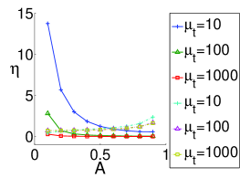
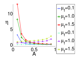
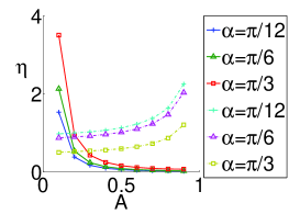
Figure 5: Cost of locomotion versus $A$ with various $\mu_{t}$, $\mu_{f}$ and $\alpha$. (a) $\eta$ vs. $A$ with various $\mu_{t}$ and fixed $\alpha=\pi/4$ and $\mu_{f}=1$. (b) $\eta$ vs. $A$ with various $\mu_{f}$ and fixed $\alpha=\pi/4$ and $\mu_{t}=30$. (c) $\eta$ vs. $A$ with various $\alpha$ and fixed $\mu_{t}=100$ and $\mu_{f}=1$. The solid lines show the cost due to transverse friction and the dashed lines denote the cost due to tangential friction.

In figure 5a, the sums of the costs of the frictional forces become smaller as $\mu_{t}$ increases. Thus the optimal $\eta$ decreases as well as shown in figure 4b. For a given motion (a given A), the slope of the tangential cost is almost unchanged as $\mu_{t}$ goes up, while the magnitude of the slope of the transverse cost quickly decays. The point where the two slopes balance shifts to the left at larger $\mu_{t}$. The optimal motion is thus obtained at a smaller amplitude as $\mu_{t}$ increases. We show the results only for $\alpha=\pi/4$ and $\mu_{f}=1$ in the figure panel, but the same phenomenon holds for all $\alpha$ and $\mu_{f}$. Physically, as the transverse coefficient increases, the snake can obtain the same amount of forward force from transverse friction with less deflection of the body and less slipping in the transverse direction, and the cost of the tangential friction is reduced as well due to a shorter path travelled. Thus, the total cost of locomotion $\eta$ decreases with $\mu_{t}$.

We show in figure 5b that the costs due to transverse friction and tangential friction both increase as $\mu_{f}$ increases. When the friction coefficient $\mu_{f}$ is larger, the snake of the same deflection experiences a stronger downward drag caused by tangential friction, increasing the slipping and consequently the work done against transverse friction as well. The optimal amplitude $A$ varies non-monotonically with $\mu_{f}$ as shown in figure 4c. The slopes of both costs increase with $\mu_{f}$ for given $A$. When $\mu_{f}<\tan\alpha$, the point where the two slopes are equal in magnitude shifts to smaller $A$ as $\mu_{f}$ increases. When $\mu_{f}>\tan\alpha$, the balanced point shifts to larger $A$.

In figure 5c, we fix $\mu_{t}=100$ and $\mu_{f}=1$, and vary the incline angle $\alpha$. The cost due to gravity is $\sin\alpha$ for the triangular wave motion and thus always increases with $\alpha$. Meanwhile, the tangential cost decreases with $\alpha$ while the transverse cost increases. The competition of these three costs makes $\eta$ non-monotonic with $\alpha$ as shown in figure 4d. For a given motion, the slope of the tangential cost with respect to $A$ is nearly unchanged as the incline becomes steeper. However, the magnitude of the slope of the transverse cost increases with $\alpha$, so a point with a given slope of the transverse cost shifts to larger $A$ as $\alpha$ increases. Therefore, the point where two slopes are equal and opposite shifts to the right as $\alpha$ goes up, and the optimal $A$ in figure 4a and c grows with $\alpha$.

IV SINUSOIDAL BODY SHAPE

IV.1 Numerical Method

We now consider an alternative, sinusoidal snake motion, to check the dependence of our results on the snake shape. We again determine the snake shape which minimizes $\eta$ for a given parameter set $(\mu_{t},\mu_{f},\mu_{b},\alpha)$. We consider the sinusoidal body shape

$$\kappa(s,t)=K\cos(n\pi s+2\pi t)$$ (34)

where the curvature is prescribed as a sinusoidal function with $t$-period $1$. We fix the wave number $n$ in this work and look for the optimal constant $K$ to minimize $\eta$ for a given $(\mu_{t},\mu_{f},\mu_{b},\alpha)$. Later we show that although the wave number $n$ affects the optimal value of $K$, it does not change the dependence of the optimal $K$ on the other parameters. We fix $n=6$ in this section, since for a horizontal plane, the lowest cost of locomotion is obtained in the limit of large wave numbers according to Alben (2013), and $n=6$ approximates this limit while only requiring a moderate number of grid points in arc length along the snake to discretize the equations accurately. We find the optimal $\eta$ on a sequence of one-dimensional meshes of $K$ values with decreasing spacing. Each mesh in the sequence is centered near the minimizer from the previous coarser mesh. The fourth mesh used has a mesh size of $10^{-3}$. We then use a quadratic curve to fit the data around the minimum point on the fourth mesh and obtain the optimal $K$ based on a final, fifth mesh, with mesh width $10^{-6}$. In Alben (2013) Alben used a BFGS algorithm to minimize the cost of locomotion when the curvature is described by a double-series expansion with 45 parameters. In this work we optimize over only a single parameter (the amplitude), for a given shape. We find that a direct search over the parameter space is typically fast enough since $\eta$ varies smoothly with $K$ in the regime of physically admissable, non-overlapping shapes.

The algorithm requires fast routines to evaluate $\eta$. Here we describe our numerical scheme that solves for the work, distance and cost of locomotion. Given the curvature $\kappa(s,t)$, we solve the three nonlinear equations (11)-(13) at each time step, over a period, for the three unknowns $x_{0}(t),y_{0}(t)$ and $\theta_{0}(t)$. Then we use equations (1)-(3) to compute $x(t),y(t),\theta(t)$ and obtain $d,W,$ and $\eta$ over one period.

We discretize the period interval uniformly with $m$ time points: $\{0,1/m,\cdots,1-1/m\}$. At each time, we rewrite equations (11)-(13) as equations in unknowns $\{\partial_{t}x_{0},\partial_{t}y_{0},\partial_{t}\theta_{0}\}$ by taking time derivatives on both sides. We solve for $\{\partial_{t}x_{0},\partial_{t}y_{0},\partial_{t}\theta_{0}\}$ over one period and then integrate to obtain $\{x_{0},y_{0},\theta_{0}\}$. The advantage of replacing $x_{0},y_{0}$ and $\theta_{0}$ with their time derivatives as variables is that it can reduce the numerical error in computing the discrete time derivatives and decrease the computational complexity by decoupling the large system of $3m$ equations in $3m$ unknowns into $m$ decoupled systems each containing only $3$ equations in $3$ unknowns Alben (2013).

We design a time-marching scheme which is second-order in both time and space to solve for $\{\partial_{t}x_{0},\partial_{t}y_{0},\partial_{t}\theta_{0}\}$ at each time level. At time $t=0$, we set $\{x_{0}^{0},y_{0}^{0},\theta_{0}^{0}\}$ to $\{0,0,0\}$ and solve for $\{\partial_{t}x_{0}^{0},\partial_{t}y_{0}^{0}\,\partial_{t}\theta_{0}^{0}\}$ using Newton’s method with a finite-difference Jacobian matrix as described in Alben (2013). At each time level $i$, we need $\{x_{0}^{i},y_{0}^{i},\theta_{0}^{i}\}$ to carry out the computation. We obtain an initial guess for the current position and angle by a forward Euler scheme using the previous step solutions $\{\partial_{t}x_{0}^{i-1},\partial_{t}y_{0}^{i-1},\partial_{t}\theta_{0}^{i-1}\}$ and $\{x_{0}^{i-1},y_{0}^{i-1},\theta_{0}^{i-1}\}$. We then solve for $\{\partial_{t}x_{0}^{i},\partial_{t}y_{0}^{i},\partial_{t}\theta_{0}^{i}\}$ at time $i$. Then we correct $\{x_{0}^{i},y_{0}^{i},\theta_{0}^{i}\}$ by integrating $\{\partial_{t}x_{0},\partial_{t}y_{0},\partial_{t}\theta_{0}\}$ from $t=0$ to $t=i/m$. Our method is similar to the prediction-correction algorithm for solving a system of ODEs. We can iterate the same procedure until a certain accuracy is obtained. We find that second-order temporal accuracy is achieved by only performing the above procedure once.

IV.2 Optima and other results

We first consider the parameter regime where $\mu_{t}\gg\mu_{f}$. In this region, the tangential motion is purely in the forward direction for the sinusoidal wave motion. Therefore, as for the triangular wave, the $\mu_{b}$ term drops out of the force law, and the parameter space is reduced to $\{\mu_{t},\mu_{f},\alpha\}$. We plot the optimal snake trajectory with parameters $\alpha=\pi/4$, $\mu_{f}=1$ and $\mu_{t}=10$ over one period in figure 6. The snake moves from left to right and its center of mass moves mainly along the $x$ direction.

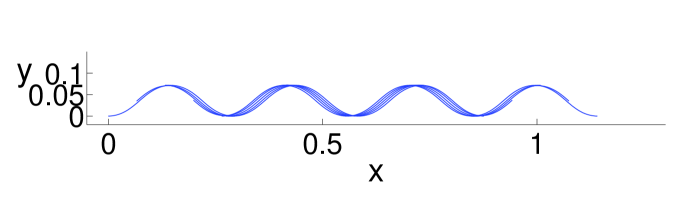
Figure 6: The optimal snake trajectory of the sinusoidal wave body shape over one period obtained with $\alpha=\pi/4$, $\mu_{f}=1$ and $\mu_{t}=10$.

$\bf{(a)}$	$\bf{(b)}$
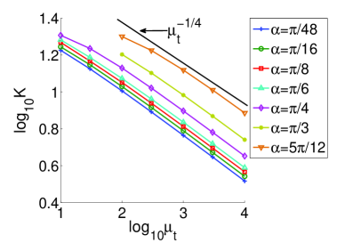
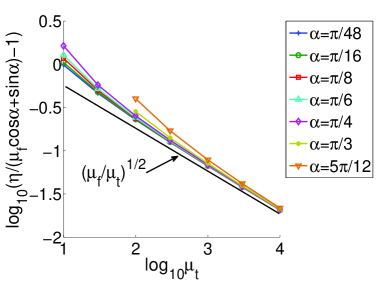
$\bf{(c)}$	$\bf{(d)}$

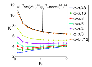
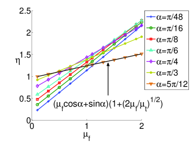
Figure 7: Scaling laws for the sinusoidal wave optima. (a) $\log_{10}K$ vs. $\log_{10}\mu_{t}$ with various $\alpha$ and fixed $\mu_{f}=1$. The solid line shows the scaling law $\mu_{t}^{-1/4}$. (b) $\log_{10}(\eta/(\mu_{f}\cos\alpha+\sin\alpha)-1)$ vs. $\log_{10}\mu_{t}$ with various $\alpha$ and fixed $\mu_{f}=1$. The solid line denotes the scaling $(\mu_{f}/\mu_{t})^{1/2}$. (c) $K$ vs. $\mu_{f}$ with various $\alpha$ and fixed $\mu_{t}=10000$. The solid line is the analytical optimum $K=\sqrt{2}n\pi(2/\mu_{t})^{1/4}(\mu_{f}^{1/2}+\tan\alpha/\mu_{f}^{1/2})^{1/2}$ obtained with $\alpha=5\pi/12.$ (d) $\eta$ vs. $\mu_{f}$ with various $\alpha$ and fixed $\mu_{t}=10000$. The solid line is the graph of the optimal $\eta=(\mu_{f}\cos\alpha+\sin\alpha)(1+(2\mu_{f}/\mu_{t})^{1/2})$ with $\alpha=5\pi/12.$

In figure 7, we vary $\mu_{t}$, $\mu_{f}$ and $\alpha$, and plot the optimal $K$ and cost of locomotion $\eta$ versus these parameters respectively. Some data points are ignored because there is no solution with non-negative $x$-velocity for the corresponding parameter values. We fix $\mu_{f}=1$ and plot the optimal $K$ and $\eta$ versus $\mu_{t}$ with various $\alpha$ in figure 7a and b. In figure 7c and d, we fix $\mu_{t}=10000$ and vary $\mu_{f}$ from $0.1$ to $2$ with different $\alpha$. We find that the optima for the sinusoidal wave motion satisfy essentially the same scaling laws as the triangular wave motion in (26) and (27). The cost of locomotion is the same as (26) and the amplitude $K$ is scaled by an extra factor $\sqrt{2}n\pi$ yielding a deflection amplitude that agrees with (27).

$\bf{(a)}$	$\bf{(b)}$	$\bf{(c)}$
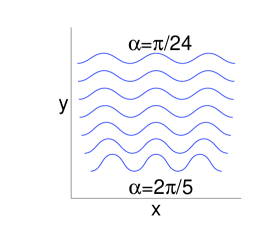
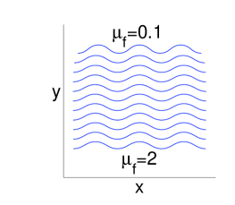
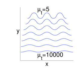
$\bf{(d)}$	$\bf{(e)}$	$\bf{(f)}$

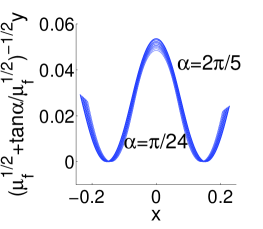
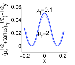
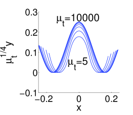
Figure 8: Optimal snake shapes at the instant $t=0$ for (a) various $\alpha$ from $\pi/24$ to $2\pi/5$ and fixed $\mu_{f}=1$ and $\mu_{t}=100$; (b) various $\mu_{f}$ from $0.1$ to $2$ and fixed $\alpha=\pi/4$ and $\mu_{t}=100$; and (c) various $\mu_{t}$ from $5$ to $10000$ and fixed $\alpha=\pi/4$ and $\mu_{f}=1$. (d) The deflection of the body rescaled by $(\mu_{f}^{1/2}+\tan\alpha/\mu_{f}^{1/2})^{-1/2}$ corresponds to (a). (e) The deflection rescaled by $(\mu_{f}^{1/2}+\tan\alpha/\mu_{f}^{1/2})^{-1/2}$ for (b). (f) The deflection rescaled by $\mu_{t}^{1/4}$ with the same parameters as (c).

In figure 8, we show the optimal snake body shapes corresponding to different $\alpha$, $\mu_{f}$ and $\mu_{t}$ in panels a, b and c respectively. We displace the different bodies vertically so that they are easier to distinguish. In figure 8d, e, and f, we rescale the deflections of the optimal shapes with $\alpha$, $\mu_{f}$, and $\mu_{t}$ according to the scaling law for the optimal amplitude (27). The centers of mass for all bodies are located at the origin. Here we zoom in on the portion of the body nearest to the center. We find a good collapse of the bodies after rescaling.

In the regime where $\mu_{t}$ and $\mu_{f}$ are comparable, the sinusoidal body shape model may not yield forward motion. For snake locomotion on a level plane, Alben Alben (2013) found that when $\mu_{t}/\mu_{f}\lesssim 6$, the optimal snake shape is no longer a retrograde traveling wave. He identified a set of locally optimal motions and classified some of them as racheting motions. When the snake climbs uphill and $\mu_{t}$ is small, the traveling wave may not be able to provide enough uphill thrust to balance gravity and the drag due to forward motion. The snake may therefore use locomotion modes other than slithering to maintain its position on the incline. For example, concertina locomotion is often observed for snakes moving inside an inclined tunnel. Marvi and Hu Marvi and Hu (2012) found that some snakes can resist sliding by lifting part of the body and reducing the contact with the ground to several localized regions. This shows that a planar model is not sufficient to describe snake locomotion on inclines when the ratio of the transverse-to-tangential friction coefficient is small. Our future work may consider three-dimensional motions to better understand this interesting parameter regime.

V Asymptotic Analysis

V.1 Optimal Shape Dynamics

We now analytically determine how the optimal snake motion depends on the parameters $\{\mu_{t},\mu_{f},\alpha\}$, thus providing theoretical confirmation of our previous results and extending them to general shapes, in the large-$\mu_{t}$ regime. We assume that the mean direction of the motion is aligned with the $x$-axis and the deflections along the $y$ direction are small, i.e. $|y|$ and all of its temporal and spatial derivatives $|\partial_{t}y|,|\partial_{s}y|,|\partial_{t}^{2}y|,\ldots,$ are $O(\mu_{t}^{\beta})$ for some negative $\beta$. We also assume that the tangential motion is only in the forward direction, to simplify the derivation. We first expand each term in the force and torque balance equations in powers of $|y|$ and retain only the terms which are dominant at large $\mu_{t}$. A detailed discussion of the expansion of each term can be found in Alben (2013). If we only keep the lowest powers in $y$ from each expression, the $x$-force balance equation becomes:

$$\int_{0}^{1}-\cos\alpha\left(\mu_{f}+\mu_{t}\partial_{s}y\left(\partial_{s}y-\frac{\partial_{t}y}{U}\right)\right)-\sin\alpha\,ds=0.$$ (35)

where $U(t)\equiv\overline{\partial_{t}x(s,t)}$ is the $s$-averaged horizontal velocity. The three terms in the integral represent the drag due to forward friction, the thrust due to transverse friction, and gravity, respectively. We note that both tangential friction and gravity forces act in the $-x$ direction, and transverse friction is essential to maintain the $x$-force balance. In Alben (2013) it is shown that for large $\mu_{t}$, a minimizer of the cost of locomotion should approximate a traveling wave motion. Therefore we pose the shape dynamics as

$$y(s,t)=g(s+U_{w}t),$$ (36)

which is a traveling wave with a prescribed wave speed $U_{w}$. $U_{w}$ is different from $U(t)$ in general, for otherwise the snake moves purely tangentially with no transverse motion. Here $g(s+U_{w}t)$ is a periodic function with period $U_{w}$. We obtain an equation for $U$ in terms of $U_{w}$ and $g$ by substituting (36) into (35):

$$-\mu_{f}\cos\alpha-\mu_{t}\cos\alpha\left(1-\frac{U_{w}}{U}\right)\langle g^{\prime}(s+U_{w}t)^{2}\rangle=\sin\alpha,$$ (37)

where $\langle g^{\prime}(s+U_{w}t)^{2}\rangle\equiv\int_{0}^{1}g^{\prime}(s+U_{w}t)^{2}\,ds$. As $\alpha\rightarrow\pi/2$, $\cos\alpha\rightarrow 0$ and no frictional force occurs. Therefore, in the limit $\alpha\rightarrow\pi/2$, we require $\mu_{t}\rightarrow\infty$ such that $\mu_{t}\cos\alpha\rightarrow\infty$, i.e, the speed at which $\alpha$ tends to $\pi/2$ depends on the speed at which $\mu_{t}$ tends to infinity. This requirement is similar to the upper bound of $\alpha$ in the triangular wave motion to obtain forward motion. As $\mu_{t}\cos\alpha\rightarrow\infty$, equation (37) holds with $(1-U_{w}/U)\rightarrow 0^{-}$. The traveling wave moves backward along the snake at speed $U_{w}$ while the snake moves forward at a speed $U$ slightly less than $U_{w}$. Therefore, the snake slips transversely to itself, which provides an uphill thrust to balance gravity and the drag due to tangential friction.

In Alben (2013) it is shown that one must expand the terms in the force balance equation in higher powers of $|y|$ to obtain an optimal motion. We do so, again assuming $y=g(s+U_{w}t)$. Then the force balance equation becomes:

$$\cos\alpha\left(\mu_{f}+\mu_{t}\left[\left(1-\frac{U_{w}}{U}\right)\langle g^{\prime}(s+U_{w}t)^{2}\rangle+\frac{1}{2}\langle g^{\prime}(s+U_{w}t)^{2}\rangle^{2}\right]\right)=-\sin\alpha,$$ (38)

and the cost of locomotion is:

$$\eta\sim\sin\alpha+\int_{0}^{1}\cos\alpha\mu_{f}(1+\frac{1}{2}\langle g^{\prime 2}\rangle)+\cos\alpha\mu_{t}\left(1-\frac{U_{w}}{U}+\frac{1}{2}\langle g^{\prime 2}\rangle\right)^{2}\langle g^{\prime 2}\rangle+O(\mu_{f}|g|^{4},\mu_{t}|g|^{8})\,dt.$$ (39)

Equation (39) is shown in a simplified form, using the result that $(1-U_{w}/U)\rightarrow 0$ as $\mu_{t}\cos\alpha\rightarrow\infty$. We substitute equation (38) into (39) and obtain:

$$\eta=1/\int_{0}^{1}\frac{1}{\displaystyle\sin\alpha+\cos\alpha\mu_{f}(1+\frac{1}{2}\langle g^{\prime 2}\rangle)+\frac{\cos\alpha(\mu_{f}+\tan\alpha)^{2}}{\mu_{t}\langle g^{\prime 2}\rangle}+O(\mu_{f}|g|^{4},\mu_{t}|g|^{8})}dt.$$ (40)

If we approximate $\langle g^{\prime}(s+U_{w}t)^{2}\rangle$ as constant in time, we obtain

$$\eta=\mu_{f}\cos\alpha+\sin\alpha+\frac{\mu_{f}\cos\alpha}{2}\langle g^{\prime 2}\rangle+\frac{\cos\alpha(\mu_{f}+\tan\alpha)^{2}}{\mu_{t}\langle g^{\prime 2}\rangle}+O(\mu_{f}|g|^{4},\mu_{t}|g|^{8}),$$ (41)

which is minimized for

$$\langle g^{\prime 2}\rangle^{1/2}=2^{1/4}\mu_{t}^{-1/4}\left(\mu_{f}^{1/2}+\frac{\tan\alpha}{\mu_{f}^{1/2}}\right)^{1/2},$$ (42)

and the corresponding optimal cost of locomotion is :

$$\eta=(\mu_{f}\cos\alpha+\sin\alpha)\left(1+\left(\frac{2\mu_{f}}{\mu_{t}}\right)^{1/2}\right).$$ (43)

In the triangular wave motion, we have

$$y(s,t)=g(s+t)=A\mathchoice{{\vbox{\hbox{$\textstyle-$ }}\kern-7.83337pt}}{{\vbox{\hbox{$\scriptstyle-$ }}\kern-5.90005pt}}{{\vbox{\hbox{$\scriptscriptstyle-$ }}\kern-4.75003pt}}{{\vbox{\hbox{$\scriptscriptstyle-$ }}\kern-4.25003pt}}\!\int\operatorname{sgn}(\sin(2\pi(s+t)))ds.$$ (44)

By using (42), we obtain that

$$A=\langle g^{\prime 2}\rangle^{1/2}=2^{1/4}\mu_{t}^{-1/4}\left(\mu_{f}^{1/2}+\frac{\tan\alpha}{\mu_{f}^{1/2}}\right)^{1/2}.$$ (45)

which is consistent with the analytical result we obtained in (27).

V.2 Optimal Curvature Analysis

For a more general body shape, to satisfy the $y$-force balance and torque balance, we instead prescribe the curvature $\kappa(s,t)$ and obtain $x(s,t)$, $y(s,t)$, and $\theta(s,t)$ from equations (1)-(3). We now correct the above analysis to satisfy all three equations. We again assume that the deflection from $x$-axis is small and we decompose $y(s,t)$ as:

$$y(s,t) = y_{0}(t)+\int_{0}^{s}\sin\theta(s^{\prime},t)ds^{\prime}$$ (46)

$$= y_{0}(t)+\int_{0}^{s}\theta(s^{\prime},t)ds^{\prime}+O(y^{3})$$ (47)

$$= y_{0}(t)+\int_{0}^{s}\theta_{0}(t)+\int_{0}^{s^{\prime}}\kappa(s^{\prime\prime},t)ds^{\prime\prime}ds^{\prime}+O(y^{3})$$ (48)

$$= y_{0}(t)+s\theta_{0}(t)+\int_{0}^{s}\int_{0}^{s^{\prime}}\kappa(s^{\prime\prime},t)ds^{\prime\prime}ds^{\prime}+O(y^{3})$$ (49)

$$\equiv Y(t)+sR(t)+k(s,t)+O(y^{3}).$$ (50)

Prescribing the curvature is the equivalent to prescribing $k(s,t)$. We set

$$k(s,t)=g(s+U_{w}t)$$ (51)

so $y$ is similar to the form given before, with two additional terms: vertical translation $Y(t)$ and rotation $R(t)$. We determine $Y$ and $R$ by expanding the $y$-force (12) and torque balance (13) equations to leading order in $|y|$ and obtain:

$$\int_{0}^{1}\left(-\frac{U_{w}}{U}+1+\frac{1}{2}\langle g^{\prime 2}\rangle\right)g^{\prime}-\frac{Y^{\prime}}{U}-\frac{R^{\prime}s}{U}+R\,ds=0,$$ (52)

$$\int_{0}^{1}s\left[\left(-\frac{U_{w}}{U}+1+\frac{1}{2}\langle g^{\prime 2}\rangle\right)g^{\prime}-\frac{Y^{\prime}}{U}-\frac{R^{\prime}s}{U}+R\right]\,ds=0.$$ (53)

We solve (52) and (53) for $Y$ and $R$:

$$\frac{Y^{\prime}}{U}-R = 4\Gamma-6\Lambda,$$ (54)

$$\frac{R^{\prime}}{U} = 12\Lambda-6\Gamma.$$ (55)

$$\Lambda \equiv \left(-\frac{U_{w}}{U}+1+\frac{1}{2}\langle g^{\prime 2}\rangle\right)\langle sg^{\prime}\rangle,$$ (56)

$$\Gamma \equiv \left(-\frac{U_{w}}{U}+1+\frac{1}{2}\langle g^{\prime 2}\rangle\right)\langle g^{\prime}\rangle.$$ (57)

We then express the $x$-force balance equation in terms of $Y$ and $R$ and obtain:

$$\int_{0}^{1}-\cos\alpha\left[\mu_{f}+\mu_{t}\left(-\frac{U_{w}}{U}+1+\frac{1}{2}\langle g^{\prime 2}\rangle\right)g^{\prime 2}+\mu_{t}\left(-\frac{Y^{\prime}}{U}-\frac{R^{\prime}s}{U}+R\right)g^{\prime}\right]-\sin\alpha\,ds=0.$$ (58)

Substituting (54) and (55) into (58) we solve for $U$ in terms of $g$:

$$\frac{U_{w}}{U}=1+\frac{1}{2}\langle g^{\prime 2}\rangle+\frac{\mu_{f}+\tan\alpha}{\displaystyle\mu_{t}\left(\langle g^{\prime 2}\rangle-\langle g^{\prime}\rangle^{2}-3(\langle g^{\prime}\rangle-2\langle sg^{\prime}\rangle)^{2}\right)}.$$ (59)

The cost of locomotion $\eta$ then becomes

$$\eta=1/\int_{0}^{1}\frac{1}{\displaystyle\sin\alpha+\cos\alpha\left(\mu_{f}\left(1+\frac{1}{2}\langle g^{\prime 2}\rangle\right)+\frac{(\mu_{f}+\tan\alpha)^{2}}{\displaystyle\mu_{t}\left(\langle g^{\prime 2}\rangle-\langle g^{\prime}\rangle^{2}-3(\langle g^{\prime}\rangle-2\langle sg^{\prime}\rangle)^{2}\right)}\right)}dt.$$ (60)

Following Alben (2013), we expand $g^{\prime}$ in a basis of Legendre polynomials $L_{k}$ for any fixed time $t$. The Legendre polynomials are orthonormal functions with unit weight on $[0,1]$. They satisfy the relations

$$\int_{0}^{1}L_{i}L_{j}ds=\delta_{ij};\ L_{0}=1,\ L_{1}=\sqrt{12}(s-1/2),\cdots$$ (61)

We write $g^{\prime}$ as:

$$g^{\prime}(s+U_{w}t)=\sum\limits_{k=0}^{\infty}c_{k}(t)L_{k}(s),$$ (62)

and we have

$$\langle g^{\prime 2}\rangle=\sum\limits_{k=0}^{\infty}c_{k}(t)^{2},$$ (63)

$$\langle g^{\prime}\rangle^{2}=c_{0}(t)^{2},$$ (64)

$$3(\langle g^{\prime}\rangle-2\langle sg^{\prime}\rangle)^{2}=c_{1}(t)^{2}.$$ (65)

Inserting into (60) we obtain

$$\eta=1/\int_{0}^{1}\frac{1}{\displaystyle\cos\alpha\left(1+\frac{1}{2}\left(c_{0}(t)^{2}+c_{1}(t)^{2}+\sum\limits_{k=2}^{\infty}c_{k}(t)^{2}\right)+\frac{(\mu_{f}+\tan\alpha)^{2}}{\mu_{t}\sum\limits_{k=2}^{\infty}c_{k}(t)^{2}}\right)+\sin\alpha}dt.$$ (66)

Therefore, $\eta$ is minimized for

$$c_{0}(t)=0;\ c_{1}(t)=0;\ \sum\limits_{k=2}^{\infty}c_{k}(t)^{2}=\sqrt{2}\mu_{t}^{-1/2}\left(\mu_{f}^{1/2}+\frac{\tan\alpha}{\mu_{f}^{1/2}}\right)$$ (67)

If a periodic function $g(s+U_{w}t)$ satisfies (67) for all $t$, this is the curvature function which minimizes the cost of locomotion. The corresponding cost of locomotion is:

$$\eta\longrightarrow(\mu_{f}\cos\alpha+\sin\alpha)\left(1+\left(\frac{2\mu_{f}}{\mu_{t}}\right)^{1/2}\right).$$ (68)

Finally, we define the amplitude of the snake motion as

$$A\equiv\left(\frac{1}{U_{w}}\int_{0}^{U_{w}}g^{\prime}(x)^{2}dx\right)^{1/2}.$$ (69)

Then we obtain that:

$$\langle g^{\prime 2}\rangle = A^{2}+O(U_{w}),$$ (70)

$$\langle g^{\prime}\rangle = O(U_{w}),$$ (71)

$$\langle sg^{\prime}\rangle = O(U_{w}).$$ (72)

Therefore, in the limit of $U_{w}\rightarrow 0$, (67) holds with the optimal

$$A=2^{1/4}\mu_{t}^{-1/4}\left(\mu_{f}^{1/2}+\frac{\tan\alpha}{\mu_{f}^{1/2}}\right)^{1/2}.$$ (73)

The derivation of (70)-(72) can be found in an appendix of Alben (2013). We notice that when $\alpha=0$ and $\mu_{f}=1$, $\eta\rightarrow 1+\sqrt{2}\mu_{t}^{-1/2}$ and the optimal $A\rightarrow 2^{1/4}\mu_{t}^{-1/4}$, which are consistent with the optimal solutions of snake motion on a level plane, derived in Alben (2013).

For the sinusoidal wave motion, we prescribed the curvature of the sinusoidal wave as

$$\kappa(s,t)=K\cos(n\pi s+2\pi t),$$ (74)

and according to (69), we obtain the amplitude $A$

$$A=\frac{K}{\sqrt{2}n\pi}.$$ (75)

Therefore, the magnitude of the sinusoidal wave $K$ scales as

$$K=(\sqrt{2}n\pi)(2^{1/4}\mu_{t}^{-1/4})\left(\mu_{f}^{1/2}+\frac{\tan\alpha}{\mu_{f}^{1/2}}\right)^{1/2}.$$ (76)

which is consistent with our numerical results.

We now discuss the case in which the snake’s net displacement is not solely in the $x$ direction, up the incline, but instead has a nonzero component in the $y$ direction, across the incline. The above analysis and Alben (2013) show that in the limit of large $\mu_{t}$, the minimum cost of locomotion is achieved when the curvature is any traveling wave function, in the limit of vanishing wavelength, and with amplitude tending to zero like $\mu_{t}^{-1/4}$. For all such optimal motions, the snake moves along a straight-line path. Let the distance travelled by the center of mass over one period be $d$, with $x$- and $y$-displacements $d_{x}$ and $d_{y}$, so $d=\sqrt{d_{x}^{2}+d_{y}^{2}}$. We may redefine $\eta$ as $W/d_{x}$ now, so only the distance travelled up the incline is considered useful. We also set $\eta=+\infty$ if $d_{x}<0$, to avoid the trivial case in which the snake travels down the incline, which we discussed in Section II. Our previous results continue to hold with this definition of $\eta$, because we set the initial orientation of the snake so that its center of mass travels only in the $x$ direction and $d=d_{x}\geq 0$ in all cases. Now if $d_{y}\geq 0$, we first claim that the optimal motions in the large-$\mu_{t}$ limit still follow straight-line paths. Any non-straight path with the same beginning and end points would have a greater arc length, and thus require more work done against forward friction for the same distance travelled by the snake’s center of mass. For a straight-line path, the work against transverse friction vanishes (corresponding to $\eta$ in equation (43) in the limit of large $\mu_{t}$), so it could not be decreased for the non-straight path. Work against gravity is the same for the straight and non-straight paths since $d_{x}$ is the same. Therefore, the straight-line path is the optimal path to minimize $\eta$. Now we show that the $\eta$-minimizing path is a straight-line path with $d_{y}=0$. $\eta$ is now a generalized version of equation (43):

$$\eta\rightarrow\mu_{f}\cos\alpha\frac{d}{dx}+\sin\alpha,\quad\mbox{as}\quad\mu_{t}\rightarrow\infty,$$ (77)

and it is minimized when $d_{y}=0$ and $d=d_{x}$. In short, nonzero $d_{y}$ increases the work against forward tangential friction without any compensating increase in $d_{x}$, so $\eta$ increases.

VI CONCLUSION

We have studied the optimization of the snake motions on an inclined plane. We used a two-dimensional model and determined the effects of the parameters—the transverse and tangential coefficients of friction and the incline angle—on the optimal shape for triangular wave motion and sinusoidal wave motion. When the transverse friction coefficient is much larger than the tangential friction coefficient, we showed that for a given incline angle $\alpha$ and tangential friction coefficient $\mu_{f}$, the cost of locomotion tends to $(\mu_{f}\cos\alpha+\sin\alpha)$ with the optimal amplitude scaling as $\mu_{t}^{-1/4}$. Our analysis also showed a non-monotonic relationship between the cost of locomotion and the incline angle. The least efficient optimal motion is achieved at a critical incline angle depending on the value of $\mu_{f}$. The optimal amplitude increases with the incline angle to decrease slipping. For given $\mu_{t}$ and $\alpha$, the motion becomes less efficient as $\mu_{f}$ increases due to the extra work against tangential friction. However, when $\mu_{f}$ is small, we find that motion with a larger amplitude is more efficient, while when $\mu_{f}$ is large, a motion with smaller amplitude is optimal. We gave an asymptotic analysis allowing a more general class of motions and our asymptotic results showed the same scaling laws for optimal amplitude and cost of locomotion.

An extension of this work is to discuss three-dimensional motions of snakes and include wider parameter spaces with small or moderate transverse friction coefficients. Another interesting direction is to consider motions in the presence of walls Marvi and Hu (2012); Maneewarn and Maneechai (2009); Transeth et al. (2008).

References

- Astley and Jayne (2007) H. Astley and B. Jayne, “Effects of perch diameter and incline on the kinematics, performance and modes of arboreal locomotion of corn snakes (elaphe guttata),” Journal of Experimental Biology 210, 3862–3872 (2007).
- Hu et al. (2009) D. Hu, J. Nirody, T. Scott, and M. Shelley, “The mechanics of slithering locomotion,” Proceedings of the National Academy of Sciences 106, 10081–10085 (2009).
- Maneewarn and Maneechai (2009) T. Maneewarn and B. Maneechai, “Design of pipe crawling gaits for a snake robot,” in Robotics and Biomimetics, 2008. ROBIO 2008. IEEE International Conference on (IEEE, 2009) pp. 1–6.
- Gray and Lissmann (1950) J Gray and HW Lissmann, “The kinetics of locomotion of the grass-snake,” Journal of Experimental Biology 26, 354–367 (1950).
- Jayne (1986) Bruce C Jayne, “Kinematics of terrestrial snake locomotion,” Copeia , 915–927 (1986).
- Shine et al. (2003) R. Shine, H. Cogger, R. Reed, S. Shetty, and X. Bonnet, “Aquatic and terrestrial locomotor speeds of amphibious sea-snakes (serpentes, laticaudidae),” Journal of zoology 259, 261–268 (2003).
- Socha (2002) John J Socha, “Kinematics: Gliding flight in the paradise tree snake,” Nature 418, 603–604 (2002).
- Erkmen et al. (2002) I. Erkmen, A. Erkmen, F. Matsuno, R. Chatterjee, and T. Kamegawa, “Snake robots to the rescue!” Robotics & Automation Magazine, IEEE 9, 17–25 (2002).
- Yim et al. (2003) M. Yim, K. Roufas, D. Duff, Y. Zhang, C. Eldershaw, and S. Homans, “Modular reconfigurable robots in space applications,” Autonomous Robots 14, 225–237 (2003).
- Hatton and Choset (2010) Ross L Hatton and Howie Choset, “Sidewinding on slopes,” in Robotics and Automation (ICRA), 2010 IEEE International Conference on (2010) pp. 691–696.
- Marvi and Hu (2012) H. Marvi and D. Hu, “Friction enhancement in concertina locomotion of snakes,” Journal of The Royal Society Interface 9, 3067–3080 (2012).
- Transeth et al. (2008) A. Transeth, R.I Leine, C. Glocker, K. Pettersen, and P. Liljeback, “Snake robot obstacle-aided locomotion: modeling, simulations, and experiments,” Robotics, IEEE Transactions on 24, 88–104 (2008).
- Hu and Shelley (2012) D. Hu and M. Shelley, “Slithering locomotion,” Natural Locomotion in Fluids and on Surfaces , 117–135 (2012).
- Jing and Alben (2013) F. Jing and S. Alben, “Optimization of two-and three-link snakelike locomotion,” Physical Review E 87, 022711 (2013).
- Alben (2013) Silas Alben, “Optimizing snake locomotion in the plane,” Proceedings of the Royal Society A 469 (2013).
- Hirose (1993) S Hirose, “Biologically inspired robots: Snake-like locomotors and manipulators,” (1993).
- Hatton et al. (2013) R. Hatton, Y. Ding, H. Choset, and D. Goldman, “Geometric visualization of self-propulsion in a complex medium,” Physical Review Letters 110, 07810 (2013).
- Ding et al. (2012) Y. Ding, S. Sharpe, A. Masse, and D. Goldman, “Mechanics of undulatory swimming in a frictional fluid,” PLoS computational biology 8, e1002810 (2012).