Energy spectrum of bottom- and charmed-flavored mesons from polarized top quark decay $t(\uparrow)\rightarrow W^{+}+B/D+X$ at ${\cal O}(\alpha_{s})$

Abstract

We consider the decay of a polarized top quark into a stable $W^{+}$ boson and charmed-flavored (D) or bottom-flavored (B) hadrons, via $t(\uparrow)\rightarrow W^{+}+D/B+X$. We study the angular distribution of the scaled-energy of B/D-hadrons at next-to-leading order (NLO) considering the contribution of bottom and gluon fragmentations into the heavy mesons B and D. To obtain the energy spectrum of B/D-hadrons we present our analytical expressions for the parton-level differential decay widths of $t(\uparrow)\rightarrow b+W^{+}(+g)$ at NLO. Comparison of our predictions with data at the LHC enable us to test the universality and scaling violations of the B- and D-hadron fragmentation functions (FFs). These can also be used to determine the polarization states of top quarks and since the energy distributions depend on the ratio $m_{W}/m_{t}$ we advocate the use of such angular decay measurements for the determination of the top quark’s mass.

I INTRODUCTION

The top quark is the heaviest particle of the Standard Model (SM) of elementary particle physics and its short lifetime implies that it decays before hadronization takes place, therefore it retains its full polarization content when it decays. This allows one to study the top spin state using the angular distributions of its decay products. Highly polarized top quarks become available at hadron colliders through single top production processes, which occurs at the $33\%$ level of the $t\bar{t}$ pair production rate Mahlon:1996pn . Near maximal and minimal values of top quark polarization at a linear $e^{+}e^{-}$ collider can be achieved in $t\bar{t}$ production by tuning the longitudinal polarization of the beam polarization Groote:2010zf so that a polarized linear $e^{+}e^{-}$ collider may be viewed as a copious source of close to zero and close to $100\%$ polarized top quarks. A first study of polarization in $t\bar{t}$ events was performed by the $D0$ collaboration Abazov:2012oxa which showed good agreement between the SM prediction and data.
The top quark total width, $\Gamma_{t}$, is proportional to the third power of its mass and is much larger than the typical QCD scale $\Lambda_{QCD}$. Therefore it enables us to treat the top quark almost as a free particle and to apply perturbative methods to evaluate the quantum corrections to its decay process.
The Large Hadron Collider (LHC) is a formidable top factory which is designed to produce about 90 million top quark pairs per year of running at design c.m. energy $\sqrt{S}=14$ TeV and design luminosity $10^{34}cm^{-2}s^{-1}$ in each of the four experiments Moch:2008qy . This will allow one to specify the properties of the top quark, such as its total decay width $\Gamma_{t}$, mass $m_{t}$ and branching fractions to high accuracy. The theoretical aspects of top quark physics at the LHC are summarized in Bernreuther:2008ju .
Due to the element $|V_{tb}|=0.999152$ of the CKM Cabibbo:1963yz quark mixing matrix, top quarks almost exclusively decay to bottom quarks, via $t\rightarrow bW^{+}$ followed by bottom quarks hadronization, $b\rightarrow H_{b}+X$, before b-quarks decay. Here, $H_{b}$ stands for the observed final state hadron fragmented from the b-quark so that its production process regarded as the nonperturbative aspect of $H_{b}$-hadron formation from top decays. Of particular interest are the distribution in the scaled $H_{b}$-hadron energy $x_{H}$ in the top quark rest frame as reliably as possible. In Ref. Kniehl:2012mn we have calculated the doubly differential distribution $d^{2}\Gamma/(dx_{B}d\cos\theta)$ of the partial width of the decay $t\rightarrow bW^{+}\rightarrow Be^{+}\nu_{e}+X$ where $\theta$ is the decay angle of the positron in the W-boson rest frame and $x_{B}$ is the scaled-energy of bottom-flavored hadrons B. In Ref. MoosaviNejad:2011yp , we also evaluated the first order QCD corrections to the energy distribution of B-hadrons from the decay of an unpolarized top quark into a charged-Higgs boson, via $t\rightarrow bH^{+}\rightarrow BH^{+}+X$, in the theories beyond-the-SM with an extended Higgs sector. In Ref. Ali:2011qf , is mentioned that a clear separation between the decay modes $t\rightarrow bW^{+}$ and $t\rightarrow bH^{+}$ can be achieved in both the $t\bar{t}X$ pair production and the $t/\bar{t}X$ single top production at the LHC.
Since bottom quarks hadronize before they decay, the particular purpose of this paper is the evaluation of the NLO QCD corrections to the energy distribution of charmed-flavored (D) and bottom-flavored (B) hadrons from the decay of a polarized top quark into a bottom quark, via $t(\uparrow)\rightarrow W^{+}+b(\rightarrow B/D+X)$ where D stands for one of the mesons $D^{0}$, $D^{+}$ and $D^{\star+}$. These measurements will be important to deepen our understanding of the nonperturbative aspects of D- and B-mesons formation which are described by realistic and nonperturbative fragmentation functions (FFs). The $b\rightarrow B$ FF is obtained through a global fit to $e^{+}e^{-}$ data from CERN LEP1 and SLAC SLC in Ref. Kniehl:2008zza and the $b\rightarrow D^{0}/D^{+}/D^{\star+}$ FFs are determined in Kneesch:2007ey by fitting the $e^{+}e^{-}$ experimental data from the BELLE, CLEO, OPAL and ALEPH collaborations. As was demonstrated in Kniehl:2012mn , the finite-$m_{b}$ corrections are rather small and thus to study the distributions in the heavy meson scaled-energy ($x_{B}$ for B-meson and $x_{D}$ for D-mesons), we employ the massless scheme or zero-mass variable-flavor-number (ZM-VFN) scheme jm in the top quark rest frame, where the zero mass parton approximation is also applied to the bottom quark. The non-zero value of the b-quark mass only enter through the initial condition of the nonperturbative FF.

This paper is structured as follows. In Sec. II, we introduce the angular structure of differential decay width by defining the technical details of our calculations. In Sec. III, our analytic results for the ${\cal O}(\alpha_{s})$ QCD corrections to the angular distributions of partial decay rates are presented. In Sec. IV, we present our numerical analysis. In Sec. V, our conclusions are summarized.

II ANGULAR DECAY DISTRIBUTION

In this section we explain the ${\cal O}(\alpha_{s})$ radiative corrections to the partial decay rate $t(\uparrow)\rightarrow W^{+}+b$. The dynamics of the current-induced $t\rightarrow b$ transition is depicted in the hadron tensor $H^{\mu\nu}$ which is introduced by

$$H^{\mu\nu} = (2\pi)^{3}\sum_{X_{b}}\int d\Pi_{f}\delta^{4}(p_{t}-p_{W}-p_{X_{b}})$$

$$\times\frac{1}{2m_{t}}<t(p_{t},s_{t})|J^{\nu+}|X_{b}><X_{b}|J^{\mu}|t(p_{t},s_{t})>,$$

where $d\Pi_{f}$ refers to the Lorentz-invariant phase space factor. In the SM the weak current is given by $J^{\mu}\propto\bar{q_{b}}\gamma^{\mu}(1-\gamma_{5})\bar{q_{t}}$. Since we are not summing over the top quark spin the hadron tensor $H^{\mu\nu}$ also depends on the top spin $s_{t}$. In this work we shall be concerned only with two types of intermediate state in Eq. (II), i.e. $|X_{b}>=|b>$ for Born term and ${\cal O}(\alpha_{s})$ one-loop contributions and $|X_{b}>=|b+g>$ for ${\cal O}(\alpha_{s})$ tree graph contribution. The decay $t(\uparrow)\rightarrow W^{+}+b$ is analyzed in the rest frame of the top quark (Fig. 1) where the three-momentum of the $b$-quark points into the direction of the positive z-axis. The polar angle $\theta_{P}$ is defined as the angle between the top quark polarization vector $\vec{P}$ and the z-axis. We shall closely follow the notation of Kniehl:2012mn where we discussed the ${\cal O}(\alpha_{s})$ radiative corrections to the partial decay rate of unpolarized top quarks.

The angular distribution of the top quark differential decay width $d\Gamma/dx$ is given by the following simple expression to clarify the correlations between the top quark decay products and the top spin

$$\frac{d^{2}\Gamma}{dx_{b}d\cos\theta_{P}}=\frac{1}{2}(\frac{d\Gamma^{unpol}}{dx_{b}}+P\frac{d\Gamma^{pol}}{dx_{b}}\cos\theta_{P}),$$ (2)

where we have defined the b-quark scaled-energy as

$$x_{b}=\frac{2E_{b}}{m_{t}(1-\omega)},$$ (3)

that $\omega$ being $\omega=m_{W}^{2}/m_{t}^{2}$. Neglecting the b-quark mass one has $0\leq x_{b}\leq 1$. In Eq. (2), P is the magnitude of the top quark polarization with $0\leq P\leq 1$ such that $P=0$ corresponds to an unpolarized top quark and $P=1$ corresponds to $100\%$ top quark polarization. $d\Gamma^{unpol}/dx_{b}$ and $d\Gamma^{pol}/dx_{b}$ stand for the unpolarized and polarized differential rates, respectively. In the following we discuss the technical details of our calculation for the ${\cal O}(\alpha_{s})$ radiative corrections to the tree-level decay rate of $t(\uparrow)\rightarrow b+W^{+}$ using dimensional regularization.

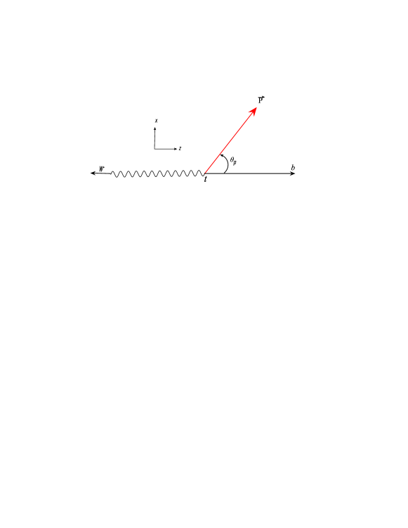
Figure 1: Definition of the polar angle $\theta_{P}$ in the top quark rest frame. $\vec{P}$ is the polarization vector of the top quark.

II.1 BORN TERM RESULTS

The Born term tensor is calculated by squaring the Born term amplitude which is given by

$$M_{0}=\frac{-eV_{tb}}{2\sqrt{2}\sin\theta_{W}}\bar{u}(p_{b},s_{b})\gamma^{\mu}(1-\gamma_{5})u(p_{t},s_{t})\epsilon^{\star}_{\mu}(p_{W},\lambda),$$

where $\epsilon^{\mu}$ stands for the W-boson polarization vector, the angle $\theta_{W}$ is the weak mixing angle and we take $\sin^{2}\theta_{W}=0.23124$ Caso:1998tx , $s$ and $p$ stand for the spin and four-momenta of particles, respectively. The squared Born amplitude is expressed as

$$|M_{0}|^{2} = \sum_{s_{b},s_{W}}M_{0}.M_{0}^{\dagger}=\frac{e^{2}}{2\sin^{2}\theta_{W}}[p_{b}.p_{t}-m_{t}p_{b}.s_{t}+$$

$$\frac{2}{m^{2}_{W}}(p_{b}.p_{W})(p_{t}.p_{W})-2\frac{m_{t}}{m_{W}^{2}}(p_{b}.p_{W})(p_{W}.s_{t})],$$

where we replaced $\sum_{s_{t}}u(p_{t},s_{t})\bar{u}(p_{t},s_{t})=(\displaystyle{\not}p_{t}+m_{t})$ in the unpolarized Dirac string by $u(p_{t},s_{t})\bar{u}(p_{t},s_{t})=1/2(1-\gamma_{5}\displaystyle{\not}s_{t})(\displaystyle{\not}p_{t}+m_{t})$ in the polarized state.
Considering Fig. 1, we parameterize the four-momenta and the polarization vector in the top rest frame as

$$p_{b} = (E_{b},0,0,E_{b}),\quad\quad\quad p_{W}=(E_{W},0,0,-E_{b}),$$

$$s_{t}=P(0,\sin\theta_{P}\cos\phi_{P},\sin\theta_{P}\sin\phi_{P},\cos\theta_{P}),$$

where the parameter P is the degree of polarization. Therefore, the LO amplitude squared reads

$$|M_{0}|^{2}=\frac{\pi\alpha}{\sin^{2}\theta_{W}}\frac{1-\omega}{\omega}m_{t}^{2}[1+2\omega+P(1-2\omega)\cos\theta_{p}].$$

Here $\pi\alpha/\sin^{2}\theta_{W}$ is related to the Fermi’s constant $G_{F}$ as $\sqrt{2}m_{W}^{2}G_{F}$.
The decay rate of a particle with a mass $m$ and momentum $p$ into a given final state of particles $(p_{1},p_{2},\cdots,p_{n})$ is

$$d\Gamma =$$

$$\frac{1}{2m}\prod_{i=1}^{n}\frac{d^{3}p_{i}}{(2\pi)^{3}}\frac{1}{2E_{i}}(2\pi)^{4}\delta^{4}(p-\sum_{i=1}^{n}p_{i})|M(m\rightarrow\{p_{i}\})|^{2},$$

$$=\frac{1}{2m}\frac{1}{(2\pi)^{3n-4}}dR_{n}(p,p_{1},p_{2},\cdots,p_{n})|M(m\rightarrow\{p_{i}\})|^{2},$$

that in the two-body phase space (e.g. $t\rightarrow b+W^{+}$), using the following relation

$$\int\frac{d^{3}\vec{p}}{2E}=\int d^{4}p\delta(p^{2}-m^{2})\Theta(E),$$ (9)

one has

$$dR_{2}(p_{t},p_{b},p_{W})=\frac{1-\omega}{8}(2\pi d\cos\theta_{P}).$$ (10)

Substituting (II.1) and (10) into (II.1), one has

$$\frac{d\Gamma_{0}}{d\cos\theta_{P}}=\frac{1}{2}\{\Gamma^{unpol}_{0}+P\Gamma^{pol}_{0}\cos\theta_{P}\},$$ (11)

where the polarized and unpolarized Born term rates read

$$\Gamma^{unpol}_{0}=\frac{m_{t}^{3}G_{F}}{8\sqrt{2}\pi}(1+2\omega)(1-\omega)^{2},$$ (12)

and

$$\Gamma^{pol}_{0}=\frac{m_{t}^{3}G_{F}}{8\sqrt{2}\pi}(1-2\omega)(1-\omega)^{2}.$$ (13)

The polarization asymmetry $\alpha_{W}$ is defined by $\alpha_{W}=\Gamma_{0}^{pol}/\Gamma_{0}^{unpol}$ which is simplified to $\alpha_{W}=(1-2\omega)/(1+2\omega)=0.396$ if we set $m_{W}=80.399$ GeV and $m_{t}=172.9$ GeV Nakamura:2010zzi .

II.2 ONE-LOOP CONTRIBUTION

The virtual one-loop contributions to the fermionic (V-A) transitions have a long history. Since at the one-loop level, QED and QCD have the same structure then the history even dates back to QED times. In this section we will investigate the one-loop corrections and describe the method applied to extract the singularities at zero-mass scheme. In the ZM-VFN scheme, where $m_{b}=0$ is set right from the start, both the soft and collinear singularities are regularized by dimensional regularization in $D=4-2\epsilon$ space-time dimensions to become single poles in $\epsilon(0<\epsilon\leq 1)$. These singularities are subtracted at factorization scale $\mu_{F}$ and absorbed into the bare FFs according to the modified minimal-subtraction $(\overline{MS})$ scheme. This renormalizes the FFs and creates in $d\Gamma/dx_{b}$ finite terms including the term $\alpha_{S}\ln(\mu_{F}^{2}/m_{t}^{2})$ which are rendered perturbatively small by choosing $\mu_{F}={\cal O}(m_{t})$.

Figure 2: Virtual (a, b) and real gluon (c, d) contributions to $t(\uparrow)\rightarrow b+W^{+}$ at NLO.

The virtual contributions exhibit both the infrared (IR) and ultraviolet (UV) singularities which are regularized in D-dimensions. To evaluate the one-loop contributions to $t(\uparrow)\rightarrow b+W^{+}$ we consider the Feynman diagrams drawn in Fig. 2. The renormalized amplitude of the virtual corrections can be written as

$$M_{loop}=\frac{-e}{2\sqrt{2}\sin\theta_{W}}\epsilon^{\star}_{\mu}(p_{W})\bar{u}(p_{b},s_{b})\{\Lambda_{\mu}+\delta\Lambda_{\mu}\}u(p_{t},s_{t}).$$

Considering Fig. 2a, the counter term of the vertex is given by $\delta\Lambda_{\mu}=(\delta Z_{b}/2+\delta Z_{t}/2)\gamma_{\mu}(1-\gamma_{5})$ where the wave-function renormalization constants of the top ($\delta Z_{t}$) and bottom ($\delta Z_{b}$) can be found in MoosaviNejad:2011yp . From Fig. 2b, for the one-loop vertex correction one has

$$\Lambda_{\mu}=\frac{C_{F}\alpha_{S}}{4i\pi^{3}}\int d^{4}p_{g}\frac{\gamma^{\beta}(\displaystyle{\not}p_{b}+\displaystyle{\not}p_{g})\gamma_{\mu}(1-\gamma_{5})(\displaystyle{\not}p_{t}+m_{t})\gamma_{\beta}}{p_{g}^{2}(p_{b}+p_{g})^{2}(p_{t}^{2}-m_{t}^{2})},$$

where $C_{F}=4/3$ stands for the color factor and $p_{g}$ refers to the gluon four-momenta. The integral (II.2) is both ir- and uv-divergent that we use dimensional regularization to extract singularities taking the replacement

$$\int\frac{d^{4}p_{g}}{(2\pi)^{4}}\rightarrow\mu^{4-D}\int\frac{d^{D}p_{g}}{(2\pi)^{D}}.$$ (16)

At ${\cal O}(\alpha_{s})$ the full amplitude is the sum of the amplitudes of the Born term, virtual one-loop and the real contributions

$$M=M_{0}+M_{loop}+M_{real}.$$ (17)

Squaring the full amplitude we have

$$|M|^{2}=|M_{0}|^{2}+|M_{vir}|^{2}+|M_{real}|^{2}+{\cal O}(\alpha_{s}^{2}),$$ (18)

where $|M_{vir}|^{2}=2M_{0}^{\dagger}M_{loop}$ and $|M_{real}|^{2}=M_{real}^{\dagger}M_{real}$. Considering Eqs. II.1 and 10, the virtual corrections to the doubly differential decay rate is then given by

$$\frac{d^{2}\Gamma_{vir}}{dx_{b}d\cos\theta_{P}}=\frac{1-\omega}{32\pi m_{t}}|M_{vir}|^{2}\delta(1-x_{b}),$$ (19)

where $x_{b}$ is defined in (3). The one-loop vertex correction and the wave-function renormalization contain uv- and ir-singularities that all uv-singularities are canceled after summing all virtual corrections up whereas the ir-divergences are remaining which are now labeled by $\epsilon$. Therefore, the virtual doubly differential distribution reads

$$\frac{d^{2}\Gamma_{vir}}{dx_{b}d\cos\theta_{P}}=\frac{1}{2}(\frac{d\Gamma^{unpol}_{vir}}{dx_{b}}+P\frac{d\Gamma^{pol}_{vir}}{dx_{b}}\cos\theta_{P}),$$ (20)

where the unpolarized differential decay rate normalized to the unpolarized Born term is

$$\frac{1}{\Gamma^{unpol}_{0}}\frac{d\Gamma^{unpol}_{vir}}{dx_{b}} =$$

$$\frac{C_{F}\alpha_{S}}{2\pi}\{A-4\frac{1-\omega}{1-4\omega^{2}}\ln(1-\omega)\}\delta(1-x_{b}),$$

and the polarized differential width normalized to the polarized Born width reads

$$\frac{1}{\Gamma^{pol}_{0}}\frac{d\Gamma^{pol}_{vir}}{dx_{b}}=\frac{C_{F}\alpha_{S}}{2\pi}A\delta(1-x_{b}),$$ (22)

with

$$A = -\frac{1}{2}\big{(}2\ln(1-\omega)-\ln\frac{4\pi\mu_{F}^{2}}{m_{t}^{2}}+\gamma_{E}-\frac{5}{2}\big{)}^{2}+$$ (23)

$$\frac{1}{\epsilon}\big{(}2\ln(1-\omega)-\ln\frac{4\pi\mu_{F}^{2}}{m_{t}^{2}}+\gamma_{E}-\frac{5}{2}\big{)}-$$

$$\frac{1-4\omega}{1-2\omega}\ln(1-\omega)+2\ln\omega\ln(1-\omega)+2Li_{2}(1-\omega)$$

$$-\frac{1}{\epsilon^{2}}-5\frac{\pi^{2}}{12}-\frac{23}{8}.$$

Here $\gamma_{E}=0.5772\cdots$ is the Euler constant and the dilogarithmic function $Li_{2}(x)$ is defined as

$$Li_{2}(x)=-\int_{0}^{x}\frac{\ln(1-z)}{z}dz.$$ (24)

As is seen, the one-loop contribution is purely real. This can be got from an inspection of the one-loop Feynman diagram Fig. 2b, which does not accept any nonvanishing physical two-particle cut.

II.3 TREE GRAPH CONTRIBUTION

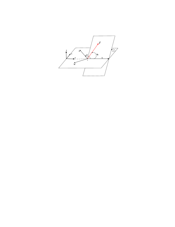
Figure 3: Definition of the azimuthal angle $\phi$ and the polar angles $\theta$ and $\theta_{P}$. $\vec{P}$ is the polarization vector of the top quark.

The ${\cal O}(\alpha_{s})$ real graph contribution results from the square of the real gluon emission graphs shown in Figs. 2(c) and 2(d). The real amplitude for the decay process $t(\uparrow)\rightarrow b(p_{b})+W^{+}(p_{W})+g(p_{g})$ reads

$$M_{real} = eg_{s}\frac{T^{n}_{ij}}{2\sqrt{2}\sin\theta_{W}}\bar{u}(p_{b},s_{b})\{\frac{\gamma^{\mu}\displaystyle{\not}p_{g}\gamma^{\beta}-2p_{t}^{\beta}\gamma^{\mu}}{2p_{t}.p_{g}}+$$

$$\frac{\gamma^{\beta}\displaystyle{\not}p_{g}\gamma^{\mu}+p_{b}^{\beta}\gamma^{\mu}}{2p_{b}.p_{g}}\}(1-\gamma_{5})u(p_{t},s_{t})\epsilon^{\star}_{\beta}(p_{g},s_{g}),$$

where $g_{s}$ is the strong coupling constant, n is the color index $(n=1,2,3,\cdots,8)$ so $Tr(T^{n}T^{n})/3=C_{F}$ and the first and second terms in the curly brackets refer to real gluon emission from the top quark and the bottom quark, respectively. The polarization vector of the gluon is denoted by $\epsilon(p_{g},s_{g})$. By working in the massless scheme, the mass of b-quark is set to zero thus the ir-divergences arise from the soft- and collinear gluon emission. As before to regulate the ir-singularities we work in D-dimensions. In the top quark rest frame (Fig. 3) the momenta and the polarization vector are defined as

$$p_{b} = E_{b}(1,0,0,1),$$

$$p_{g} = E_{g}(1,\sin\theta,0,\cos\theta),$$

$$s_{t} = P(0,\sin\theta_{P}\cos\phi_{P},\sin\theta_{P}\sin\phi_{P},\cos\theta_{P}).$$ (26)

Considering (II.1) the real differential rate in D-dimensions is given by

$$d\Gamma_{real} = \frac{1}{2m_{t}}\frac{\mu_{F}^{2(4-D)}}{(2\pi)^{2D-3}}|M_{real}|^{2}$$

$$\times\frac{d^{D-1}\vec{p}_{b}}{2E_{b}}\frac{d^{D-1}\vec{p}_{W}}{2E_{W}}\frac{d^{D-1}\vec{p}_{g}}{2E_{g}}\delta^{D}(p_{t}-p_{b}-p_{g}-p_{W}).$$

To calculate the differential decay rate $d\Gamma_{real}/dx_{b}$ normalized to the Born width, we fix the momentum of b-quark and integrate over the energy of gluon which ranges from $E_{g}^{min}=m_{t}(1-\omega)(1-x_{b})/2$ and $E_{g}^{max}=m_{t}(1-\omega)(1-x_{b})/(2(1-x_{b}(1-\omega)))$ and to obtain the angular distribution of differential width $d^{2}\Gamma_{real}/(dx_{b}d\cos\theta_{P})$, the angular integral in D-dimensions is written as

$$d\Omega_{b}=\frac{2\pi^{\frac{D}{2}-1}}{\Gamma(\frac{D}{2}-1)}(\sin\theta_{P})^{D-4}d\cos\theta_{P}.$$ (28)

In the massless scheme, the real and virtual differential widths contain the poles $\propto 1/\epsilon$ and $1/\epsilon^{2}$ which disappear only in the total NLO width. This requires that to get the correct finite terms in the normalized doubly differential distribution $1/\Gamma_{0}\times d^{2}\Gamma_{real}/(dx_{b}d\cos\theta_{P})$, the polarized and unpolarized Born widths will have to be evaluated in dimensional regularization at ${\cal O}(\epsilon^{2})$. We find

$$\Gamma_{0}^{unpol} = \frac{m_{t}^{3}G_{F}}{8\sqrt{2}\pi}(1+2\omega)(1-\omega)^{2}\bigg{\{}1+\epsilon F+\epsilon^{2}\big{[}\frac{F^{2}}{2}+$$

$$2\frac{(1+\omega)(1+3\omega)}{(1+2\omega)^{2}}-\frac{\pi^{2}}{4}\big{]}\bigg{\}},$$

$$\Gamma_{0}^{pol} = \frac{m_{t}^{3}G_{F}}{8\sqrt{2}\pi}(1-2\omega)(1-\omega)^{2}\bigg{\{}1+\epsilon\big{[}H+\frac{2\omega}{1-2\omega}\big{]}+$$

$$\epsilon^{2}\big{[}\frac{1}{2}(H+\frac{5}{2})^{2}-H\frac{5-14\omega}{2(1-2\omega)}-\frac{\pi^{2}}{12}-\frac{25}{8}\big{]}\bigg{\}},$$

with

$$F = \ln\frac{4\pi\mu_{F}^{2}}{m_{t}^{2}}-2\ln(1-\omega)-\gamma_{E}+2\frac{1+\omega}{1+2\omega},$$

$$H = \ln\frac{4\pi\mu_{F}^{2}}{m_{t}^{2}}-2\ln\frac{1-\omega}{2}-\gamma_{E}.$$ (30)

Now the real gluon contribution is given by

$$\frac{d^{2}\Gamma_{real}}{dx_{b}d\cos\theta_{P}}=\frac{1}{2}(\frac{d\Gamma^{unpol}_{real}}{dx_{b}}+P\frac{d\Gamma^{pol}_{real}}{dx_{b}}\cos\theta_{P}),$$

where, by defining $T=-\ln(4\pi\mu_{F}^{2}/m_{t}^{2})+2\ln(1-\omega)+\gamma_{E}$, one has

$$\frac{1}{\Gamma^{unpol}_{0}}\frac{d\Gamma^{unpol}_{real}}{dx_{b}} = \frac{C_{F}\alpha_{S}}{2\pi}\bigg{\{}\delta(1-x_{b})\bigg{[}\frac{1}{2}T^{2}-T+\frac{1}{\epsilon^{2}}-$$

$$\frac{2\omega}{1-\omega}\ln\omega+2Li_{2}(1-\omega)-\frac{1}{\epsilon}(T-1)$$

$$-\frac{\pi^{2}}{4}\bigg{]}+2(1+x_{b}^{2})\Big{(}\frac{\ln(1-x_{b})}{1-x_{b}}\Big{)}_{+}+$$

$$\frac{1}{(1-x_{b})_{+}}\bigg{[}1-4x_{b}+x_{b}^{2}+$$

$$\frac{4x_{b}\omega(1-\omega)(1-x_{b})^{2}}{(1+2\omega)(1-x_{b}(1-\omega))}+$$

$$(1+x_{b}^{2})\bigg{(}\ln[\frac{x_{b}^{2}(1-\omega)^{2}m_{t}^{2}}{4\pi\mu_{F}^{2}}]+$$

$$\gamma_{E}-\frac{1}{\epsilon}\bigg{)}\bigg{]}\bigg{\}},$$

and

$$\frac{1}{\Gamma^{pol}_{0}}\frac{d\Gamma^{pol}_{real}}{dx_{b}} = \frac{C_{F}\alpha_{S}}{2\pi}\bigg{\{}\delta(1-x_{b})\big{[}\frac{1}{2}T^{2}-T-\frac{2\omega}{1-\omega}\ln\omega$$

$$+2Li_{2}(1-\omega)-\frac{1}{\epsilon}(T-1)+\frac{1}{\epsilon^{2}}-\frac{\pi^{2}}{4}\big{]}$$

$$+2(1+x_{b}^{2})\Big{(}\frac{\ln(1-x_{b})}{1-x_{b}}\Big{)}_{+}+$$

$$\frac{1}{(1-x_{b})_{+}}\bigg{[}-1-x_{b}^{2}+\frac{8\omega(1-x_{b})^{2}}{1-2\omega}+$$

$$4\frac{x_{b}\omega(1-\omega)(1-x_{b})^{2}}{(1-2\omega)(1-x_{b}(1-\omega))}+$$

$$(1+x_{b}^{2})\bigg{(}\ln[\frac{x_{b}^{2}(1-\omega)^{2}m_{t}^{2}}{4\pi\mu_{F}^{2}}]+\gamma_{E}-\frac{1}{\epsilon}\bigg{)}$$

$$+\frac{8\omega(1-x_{b})^{2}}{x_{b}(1-\omega)(1-2\omega)}\ln(1-x_{b}(1-\omega))\bigg{]}\bigg{\}}.$$

III ANALYTIC RESULTS FOR ANGULAR DISTRIBUTION OF PARTIAL DECAY RATES

Now we are in a situation to present our analytic results for the angular distribution of the differential decay rate, by summing the Born-level (11), the virtual (20) and real gluon (II.3) contributions. According to the Lee-Nauenberg theorem, all singularities cancel each other after summing all contributions up and the final result is free of ir-singularities. Therefore, the complete ${\cal O}(\alpha_{s})$ results are

$$\frac{d^{2}\Gamma}{dx_{b}d\cos\theta_{P}}=\frac{1}{2}\{\frac{\Gamma^{unpol}_{Nlo}}{dx_{b}}+P\frac{d\Gamma^{pol}_{Nlo}}{dx_{b}}\cos\theta_{P}\},$$ (34)

that we presented $d\Gamma^{unpol}_{Nlo}/dx_{b}$ in Ref. Kniehl:2012mn and $d\Gamma^{pol}_{Nlo}/dx_{b}$ in the $\overline{MS}$ scheme is expressed, for the first time, as

$$\frac{1}{\Gamma^{pol}_{0}}\frac{d\Gamma^{pol}_{Nlo}}{dx_{b}} = \delta(1-x_{b})+\frac{C_{F}\alpha_{s}}{2\pi}\bigg{\{}\delta(1-x_{b})\big{[}-\frac{3}{2}\ln\frac{\mu_{F}^{2}}{m_{t}^{2}}$$

$$+2\frac{1-\omega}{1-2\omega}\ln(1-\omega)-2\frac{\omega}{1-\omega}\ln\omega-\frac{2\pi^{2}}{3}$$

$$+2\ln\omega\ln(1-\omega)+4Li_{2}(1-\omega)-6\big{]}$$

$$+2(1+x_{b}^{2})\Big{(}\frac{\ln(1-x_{b})}{1-x_{b}}\Big{)}_{+}+$$

$$\frac{1}{(1-x_{b})_{+}}\bigg{[}-1-x_{b}^{2}+\frac{8\omega(1-x_{b})^{2}}{1-2\omega}+$$

$$4\frac{x_{b}\omega(1-\omega)(1-x_{b})^{2}}{(1-2\omega)(1-xb(1-\omega))}+$$

$$(1+x_{b}^{2})\ln[x_{b}^{2}(1-\omega)^{2}\frac{m_{t}^{2}}{\mu_{F}^{2}}]+$$

$$\frac{8\omega(1-x_{b})^{2}}{x_{b}(1-\omega)(1-2\omega)}\ln(1-x_{b}(1-\omega))\bigg{]}\bigg{\}}.$$

Since the observed mesons can be also produced through a fragmenting gluon, therefore, to obtain the most accurate result for the energy spectrum of meson we have to add the contribution of gluon fragmentation to the b-quark to produce the outgoing meson. From Fig. 4, it is seen that the contribution of gluon decreases the size of decay rate up to $40\%$ at the threshold, thus this contribution can be important at low energy of the observed meson. Therefore, the differential decay rate $d\Gamma/dx_{g}$ is also required where $x_{g}$ is defined as $x_{g}=2E_{g}/(m_{t}(1-\omega))$ as in (3). To obtain the doubly differential distribution $d^{2}\Gamma/(dx_{g}d\cos\theta_{P})$, we integrate over the b-quark energy by fixing the gluon momentum in the phase space. The result is

$$\frac{d^{2}\Gamma}{dx_{g}d\cos\theta_{P}}=\frac{1}{2}\{\frac{\Gamma^{unpol}_{Nlo}}{dx_{g}}+P\frac{d\Gamma^{pol}_{Nlo}}{dx_{g}}\cos\theta_{P}\},$$ (36)

where $d\Gamma^{unpol}_{Nlo}/dx_{g}$ can be found in our previous work Kniehl:2012mn and $d\Gamma^{pol}_{Nlo}/dx_{g}$ is listed here

$$\frac{1}{\Gamma^{pol}_{0}}\frac{d\Gamma^{pol}_{Nlo}}{dx_{g}} = \frac{C_{F}\alpha_{s}}{2\pi}\bigg{\{}\frac{2}{x_{g}^{2}}\ln(1-x_{g}(1-\omega))\big{[}$$

$$\frac{(1-2x_{g})^{2}}{1-\omega}+\frac{4x_{g}(1-x_{g})}{1-2\omega}\big{]}+$$

$$\frac{1}{2(1-2\omega)}\big{[}2(1-2\omega)+\frac{4(1+\omega)}{1-\omega}-$$

$$x_{g}(1+6\omega)-\frac{\omega(6\omega^{2}+\omega+2)}{(1-\omega)(1-x_{g}(1-\omega))}$$

$$-\frac{\omega^{2}(1-2\omega)}{(1-\omega)(1-x_{g}(1-\omega))^{2}}\big{]}+$$

$$\frac{1+(1-x_{g})^{2}}{x_{g}}\big{[}2\ln(x_{g}(1-x_{g}))-\ln\frac{\mu_{F}^{2}}{m_{t}^{2}}$$

$$-\ln(1-x_{g}(1-\omega))+2\ln(1-\omega)]\bigg{\}}.$$

IV NONPERTURBATIVE FRAGMENTATION AND HADRON LEVEL RESULTS

In this section, performing a numerical analysis we present our phenomenological results for the energy spectrum of the heavy mesons B and D from polarized top decays and compare them with the unpolarized one in Kniehl:2012mn . We define the normalized-energy fractions of the outgoing mesons similarly to the parton-level one in (3) as $x_{B}=2E_{B}/(m_{t}(1-\omega))$ for the B-meson and $x_{D}=2E_{D}/(m_{t}(1-\omega))$ for the D-meson. Considering the factorization theorem of the QCD-improved parton model jc , the energy distribution of a hadron can be expressed as the convolution of the parton-level spectrum with the nonperturbative fragmentation function $D_{a}^{H}(z,\mu_{F})$

$$\frac{d\Gamma}{dx_{H}}=\sum_{i=b,g}\frac{d\Gamma}{dx_{i}}(\mu_{R},\mu_{F})\otimes D_{i}^{H}(\frac{x_{H}}{x_{i}},\mu_{F}),$$ (38)

where $H$ stands for $B-$ and $D$-mesons and the allowed $x_{H}$ ranges are $2m_{H}/(m_{t}(1-\omega))\leq x_{H}\leq 1$. The integral convolution appearing in (38) is defined as

$$(f\otimes g)(x)=\int_{x}^{1}dxf(z)g(\frac{x}{z}).$$ (39)

In (38), $\mu_{F}$ and $\mu_{R}$ are the factorization and the renormalization scales, respectively, and one can use two different values for these scales; however, a choice often made consists of setting $\mu_{R}=\mu_{F}$ and we adopt the convention $\mu_{R}=\mu_{F}=m_{t}$ for our results. In (38), $d\Gamma/dx_{i}$ are the parton-level differential rates presented in (34) and (36) and $D_{i}^{H}$ are the nonperturbative FFs describing the hadronizations $b\rightarrow H$ and $g\rightarrow H$ which are process independent. Several models have been yet proposed to describe the FFs. In Ref. Kneesch:2007ey , authors calculated the FFs for $D^{0},D^{+}$ and $D^{\star+}$ mesons by fitting the experimental data from the BELLE, CLEO, OPAL, and ALEPH collaborations in the modified minimal-subtraction ($\overline{MS}$) factorization scheme. They have parameterized the $z$ distributions of the $b\rightarrow D^{0}/D^{+}/D^{\star+}$ FFs at their starting scale $\mu_{0}=m_{b}$, as suggested by Bowler Bowler , as

$$D_{b}^{D}(z,\mu_{0})=Nz^{-(1+\gamma^{2})}(1-z)^{a}e^{-\gamma^{2}/z},$$ (40)

while the FF of the gluon is set to zero and this FF is evolved to higher scales using the DGLAP equations dglap . As in Kneesch:2007ey is claimed, this parametrization yields the best fit to the BELLE data Seuster:2005tr in a comparative analysis using the Monte-Carlo event generator JETSET/PYTHIA. The values of fit parameters together with the achieved values of $\overline{\chi^{2}}$ are presented in Table 1.

Table 1: Values of fit parameters for $b\rightarrow D^{0}$, $b\rightarrow D^{+}$ and $b\rightarrow D^{\star+}$ FFs at the starting scale $\mu_{0}=m_{b}$ resulting from the global fit in the ZM approach together with the values of $\overline{\chi^{2}}$ achieved.

	$N$	$a$	$\gamma$	$\overline{\chi^{2}}$
$D^{0}$	$80.8$	$5.77$	$1.15$	$4.66$
$D^{+}$	$163$	$6.93$	$1.40$	$2.21$
$D^{\star+}$	$14.9$	$3.87$	$1.16$	$7.64$

From Ref. Kniehl:2008zza we employ the $b\rightarrow B$ FF determined at NLO in the ZM-VFN approach through a global fit to $e^{+}e^{-}$-annihilation data taken by ALEPH Heister:2001jg and OPAL Abbiendi:2002vt at CERN LEP1 and by SLD Abe:1999ki at SLAC SLC. The power ansatz $D_{b}^{B}(z,\mu_{0})=Nz^{\alpha}(1-z)^{\beta}$ was used as the initial condition for the $b\to B$ FF at $\mu_{0}=m_{b}$, while the gluon FF was generated via the DGLAP evolution. The fit parameters are $N=4684.1$, $\alpha=16.87$, and $\beta=2.628$ with $\overline{\chi^{2}}=1.495$. Following Ref. Nakamura:2010zzi we adopt the input values $G_{F}=1.16637\times 10^{-5}$ GeV^-2, $m_{t}=172.9$ GeV, $m_{b}=4.78$ GeV, $m_{W}=80.339$ GeV, $m_{B}=5.279$ GeV, $m_{D}=1.87$ GeV, and $\Lambda_{\overline{MS}}^{(5)}=231$ MeV with $n_{f}=5$ active quark flavors and adjusted such that $\alpha_{s}^{(5)}(m_{Z}=91.18)=0.1184$.
To study the scaled-energy ($x_{B}$ and $x_{D}$) distributions of the bottom- and charmed-flavored hadrons produced in the polarized top decay, we consider the quantities $d\Gamma(t(\uparrow)\to B+X)/dx_{B}$ and $d\Gamma(t(\uparrow)\to D+X)/dx_{D}$ in the ZM-VFN scheme. In Fig. 4, our prediction for the B-meson is shown by studying the size of the NLO corrections, by comparing the LO (dotted line) and NLO (solid line) results, and the relative importance of the $b\rightarrow B$ (dashed line) and $g\rightarrow B$ (dot-dashed line) fragmentation channels at NLO. We evaluated the LO result using the same NLO FFs. The $g\rightarrow B$ contribution is negative and appreciable only in the low-$x_{B}$ region. For higher values of $x_{B}$, as is expected Corcella:2001hz , the NLO result is practically exhausted by the $b\rightarrow B$ contribution. Note that the contribution of the gluon can not be discriminated. It is calculated to see where it contributes to $d\Gamma/dx_{B}$. So this part of the paper is of more theoretical relevance. In the scaled-energy of mesons as a experimental quantity, all contributions including the b quark, gluon and light quarks contribute.

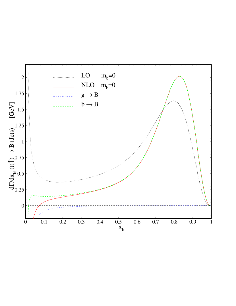
Figure 4: $d\Gamma(t(\uparrow)\to BW^{+}+X)/dx_{B}$ as a function of $x_{B}$ in the ZM-VFN ($m_{b}=0$) scheme. The NLO result (solid line) is compared to the LO one (dotted line) and broken up into the contributions due to $b\to B$ (dashed line) and $g\to B$ (dot-dashed line) fragmentation. We set $\mu_{F}=m_{t}$ and $\mu_{0F}=m_{b}$.

In Fig 5, the scaled-energy ($x_{B}$) distribution of B-hadrons produced in unpolarized (dashed line) and polarized (solid line) top quark decays at NLO are studied. As is seen, in the unpolarized top decay the partial decay width at Hadron-level is around $38\%$ higher than the one in the polarized top decay in the peak region. In Fig. 6 the same comparison is also down for the transition $b\rightarrow D^{0}$ applying the Bowler model (40) for the FFs. Fig. 6 shows that the probability to produce the charmed-flavored mesons through top quark decays in the high-$x_{D}$ range ($0.7\lesssim x_{D}$) is zero. In fig. 7 we study the scaled-energy ($x_{D}$) distribution of charmed-flavored hadrons produced in polarized top decays as $t(\uparrow)\rightarrow D^{0}+X_{1}$ (solid line), $t(\uparrow)\rightarrow D^{\star+}+X_{2}$ (dotted line) and $t(\uparrow)\rightarrow D^{+}+X_{3}$ (dashed line). Note that our results are valid just for $x_{D}\geq 2E_{D}/(m_{t}(1-\omega))=0.028$ and $x_{B}\geq 0.078$.

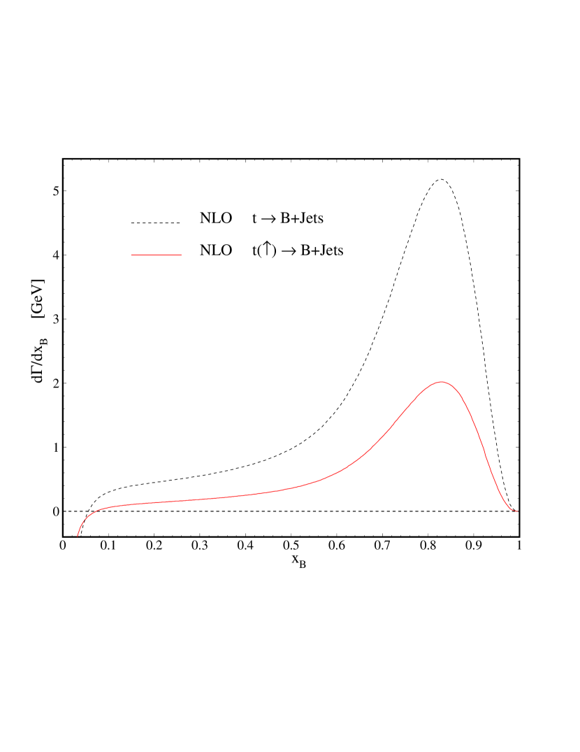
Figure 5: $d\Gamma/dx_{B}$ as a function of $x_{B}$ in the ZM-VFN ($m_{b}=0$) scheme considering the unpolarized (dashed line) and polarized (solid line) partial decay rates at NLO.

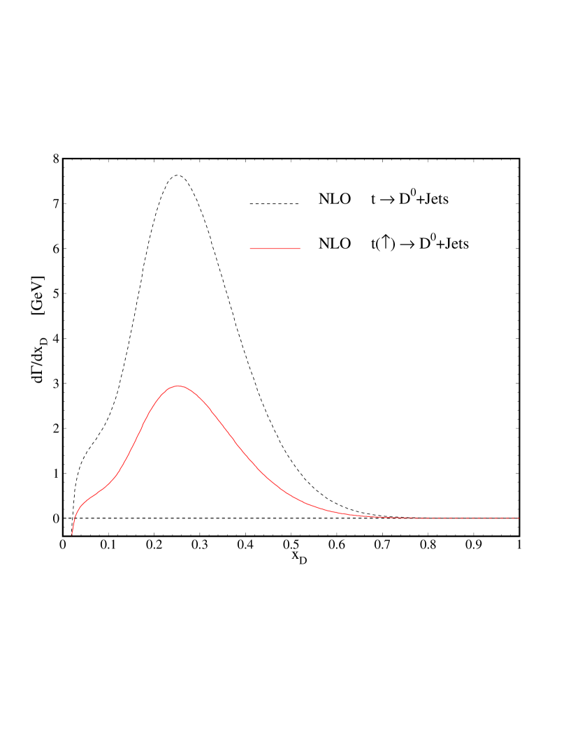
Figure 6: $x_{D}$ spectrum in top decay, with the hadronization modeled according to the Bowler model considering the unpolarized (dashed line) and polarized (solid line) decay rates at NLO. We set $\mu_{F}=m_{t}$ and $\mu_{0F}=m_{b}$.

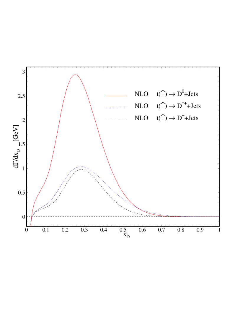
Figure 7: $d\Gamma(t(\uparrow)\to DW^{+}+X)/dx_{D}$ as a function of $x_{D}$ at NLO for $D=D^{0}$ (solid line), $D=D^{\star+}$ (dotted line) and $D=D^{+}$ (dashed line).

V Conclusions

The top quark decays rapidly so that it has no time to hadronize and passes on its full spin information to its decay products. The CERN LHC, as a superlative top factory, allows us to study top quark decays that within the SM are completely dominated by the mode $t\rightarrow W^{+}+b$, followed by $b\rightarrow H+X$. Therefore, the distribution in the scaled H-hadron energy $x_{H}$ in the top rest frame are of particular interest. In fact, the $x_{H}$ distribution provides direct access to the H-hadron FFs, and its $\cos\theta_{P}$ distribution allows one to analyze the top quark polarization where the polar angle $\theta_{P}$ refers to the angle between the polarization vector of the top and the z-axis.
In Kniehl:2012mn we have studied the scaled-energy ($x_{B}$) distribution of the B-meson in unpolarized top quark decays and in the present work we made our predictions for the scaled-energy ($x_{B},x_{D}$) distributions of the B- and D-mesons in the polarized top quark rest frame by studying the quantity $d^{2}\Gamma/(dx_{H}d\cos\theta_{P})$. As was mentioned, the scaled-energy distribution of hadron enables us to deepen our knowledge of the hadronization process and to pin down the $b,g\rightarrow B/D$ FFs while the angular analysis of the polarized top decay constrain these FFs even further. Furthermore, the polarization state of top quarks can be specified from the angular distribution of the outgoing hadron energy. The universality and scaling violations of the B- and D-hadron FFs will be able to test at LHC by comparing our NLO predictions with future measurements of $d\Gamma/dx_{H}$ and $d\Gamma(\uparrow)/dx_{H}$. One can also test the SM and/or non-SM couplings through polarization measurements involving top quark decays (mostly $t(\uparrow)\rightarrow b+W^{+}$). The formalism made here is also applicable to the production of hadron species other than B and D hadrons, such as pions and kaons, through the polarized top quark decay using the $b,g\rightarrow\pi/K$ FFs presented in our recently paper maryam .