Stability of charged thin-shell wormholes in $(2+1)$ dimensions

Abstract

In this paper we construct charged thin-shell wormholes in (2+1)-dimensions applying the cut-and-paste technique implemented by Visser, from a BTZ black hole which was discovered by Bañados, Teitelboim and Zanelli BTZ1992 , and the surface stress are determined using the Darmois-Israel formalism at the wormhole throat. We analyzed the stability of the shell considering phantom-energy or generalised Chaplygin gas equation of state for the exotic matter at the throat. We also discussed the linearized stability of charged thin-shell wormholes around the static solution.

I Introduction

Last two decades traversable wormholes and thin-shell wormholes are very interesting topic to the scientist, though it is a hypothetical concept in space-time. At first Morris and Thorns MT1988 proposed the structure of traversable wormhole which is the solution of Einstein’s field equations having two asymptotically flat regions connected by a minimal surface area, called throat, satisfying flare-out condition HV1997 . However, one has to tolerate the violation of energy condition which is treated as exotic matter. Visser, Kar and Dadhich VSD2003 have shown how one can construct a traversable wormhole with small violation of energy condition. Different types of wormholes have been discussed in LFO2003 ; L87 ; MV ; DSM .

Though, it is very difficult to deal with the exotic matter (violation of energy condition), Visser M.v1989 , adapted a way to minimize the usage of exotic matter applying the cut-and-paste technique on a black hole to construct a new class of spherically symmetric wormhole, known as thin-shell wormhole where the exotic matter is concentrated at the throat of the wormhole. The surface stress-energy tensor components, at the throat, are determined using the Darmois-Israel formalism IW ; PH .

It is needed to define an equation of state for the exotic matter, located at the throat, though several models have been proposed, one of them is the Phantom-like equation of state defined as: $p$=$w\rho$, $w<-1$, for more specifically when $w<-1/3$, then the equation of state is dark energy type and when $w>-1/3$, then equation of state is quintessence type. Another important equation of state is the generalised Chaplygin gas , defined as: $p$=$-A/\rho^{\alpha}$, where A is a positive constant and $0<\alpha\leq 1$. A well study for both equation of state on wormholes have been discussed in FSAK ; MPF ; CE ; E ; FSN ; FSN2006 ; MOA ; S ; TME ; P .

For the local stability of the shell around the static solution under small perturbation, Visser and Poission EP proposed the linearized stability analysis for thin-shell wormhole by joining two Sehwarzschild geometries. Lobo and Crawford LC , extended the idea of linearized stability analysis with the cosmological constant.Stablity analysis of charged thin-shell wormholes have been studied in ECS ; EC ; AZF ; FKS . Recently several works have been done in (2+1) dimensions in KJM2004 ; Kim2004 ; EA ; RS2011 ; FR2011 ; FAI ; MR ; MJ .

Charged black holes and wormholes are very interesting topic in recent days. Charge without charge effects of Misner-Wheeler MC is one of the most interesting fact produced by wormholes. Morris and Thorns wormhole takes a new level after the addition of an electric charged proposed by Kim and Lee SS ; SH .

In the year 1992, Bañados, Teitelboim and Zanelli (BTZ) BTZ1992 discovered a black hole in (2+1) dimensions with a negative cosmological constant, which is very similar to (3+1) dimensional black hole. Babichev, Dokuchaev and Eroshenko EV have shown that with accretion of phantom-energy, black hole mass decreases and for the decreasing mass, the existence of horizon is not crucial. Applying this concept on BTZ black hole, Jamil and Akbar MM have shown that mass evolution is dependent on the pressure and density of the phantom energy rather than the mass of the black hole.

In this work, we present a thin-shell wormhole from charged BTZ black holes by the cut-and-paste technique in (2+1)-dimensions. Here we survey, whether the charged thin-shell is stable or not when we consider the equation of state is Phantom-like or generalised Chaplygin gas. Linearized stability has also discussed around the static solution. Various aspects of the thin-shell wormholes are also analyzed.

II construction of Charged Thin-shell wormhole

The charged BTZ black hole with a negative cosmological constant $\Lambda=-1/L{{}^{2}}$ is a solution of (2+1)-dimensional gravity. The metric is given by ccj

$$ds^{2}=-f(r)dt^{2}+\frac{dr^{2}}{f(r)}+r^{2}d\phi^{2},$$ (1)

$$f(r)=\frac{r^{2}}{L{{}^{2}}}-\left[M+\frac{Q^{2}}{2}\ln(\frac{r}{L})\right].$$ (2)

Where $f(r)$ is known as lapse function. $M$ and $Q$ are mass and electric charge of the BTZ black hole. Here we take two identical copies from BTZ black hole with $r\geq a$:

$$\mathcal{M}^{\pm}=(x\mid r\geq a)$$

and stick them together at the junction surface

$$\Sigma=\Sigma^{\pm}=(x\mid r=a)$$

to get a new geodesically complete manifold $\mathcal{M}=\mathcal{M}^{+}+\mathcal{M}^{-}$. The minimal surface area at $\Sigma$, referred as a throat of wormhole where we take $a>r_{h}$ to avoid the event horizon.

The junction surface (where the wormhole throat is located) is one dimensional ring of matter where the stress energy components are non zero can be evaluated using the second fundamental formsMR ; MJ ; FAI ; EA defined by

$$K^{i\pm}_{j}=\frac{1}{2}g^{ik}\frac{\partial g_{kj}}{\partial\eta}\Bigl{\lvert}_{\eta=\pm 0}=\frac{1}{2}\frac{\partial r}{\partial\eta}\Bigl{\lvert}_{r=a}~{}g^{ik}\frac{\partial g_{kj}}{\partial r}\Bigl{\rvert}_{r=a}.$$ (3)

Here, $\eta$ is the Riemann normal coordinates, positive and negative in two side of the boundaries with $x^{\mu}=(\tau,\phi,\eta)$, where $\tau$ represents the proper time on the shell.

Since, $K_{ij}$ is not continuous for the shell around $\Sigma$, so the second fundamental forms with discontinuity are given by

$$\mathcal{K}_{ij}=K^{+}_{ij}-K^{-}_{ij}.$$ (4)

Now, one can define the surface stress energy tensor $S^{i}_{j}$, at the junction. Using Lanczos equation follow from the Einstein equations lead to

$$S^{i}_{j}=-\frac{1}{8\pi}\left(K^{i}_{j}-\delta^{i}_{j}K^{k}_{k}\right).$$ (5)

Considering circular symmetry, $K^{i}_{j}$ becomes

$$K^{i}_{j}=\left({\begin{array}[]{cc}K^{\tau}_{\tau}&0\\ 0&K^{\phi}_{\phi}\\ \end{array}}\right),$$ (6)

then the surface stress-energy tensor become

$$S^{i}_{j}=\left({\begin{array}[]{cc}-\sigma&0\\ 0&-v\\ \end{array}}\right),$$ (7)

where $\sigma$ is surface energy density and $v$ is surface pressure, then Lanczos equation becomes

$$\sigma = -\frac{1}{8\pi}\kappa_{\phi}^{\phi},$$ (8)

$$v = -\frac{1}{8\pi}\kappa_{\tau}^{\tau}.$$ (9)

Now, using the Eqs.(3-9) for the metric given in Eq.(1), we get the above expression as

$$\sigma=-\frac{1}{4\pi a}\sqrt{\frac{a^{2}}{L{{}^{2}}}-\left[M+\frac{Q^{2}}{2}\ln(\frac{a}{L})\right]+\dot{a}^{2}},$$ (10)

$$p=-v=\frac{1}{4\pi}\left[\frac{\frac{a}{r_{0}{{}^{2}}}-\frac{Q^{2}}{4a}+\ddot{a}}{\sqrt{\frac{a^{2}}{L{{}^{2}}}-\left[M+\frac{Q^{2}}{2}\ln(\frac{a}{L})\right]+\dot{a}^{2}}}\right].$$ (11)

Here, overdot denotes the derivatives with respect to $\tau$, assuming the throat radius is a function of proper time i.e. $a=a(\tau)$.

For the static configuration of radius $a$, we have (i.e. $\dot{a}=0$ and $\ddot{a}=0$) from Eqs.(10) and (11)

$$\sigma=-\frac{1}{4\pi a}\sqrt{\frac{a^{2}}{L{{}^{2}}}-\left[M+\frac{Q^{2}}{2}\ln(\frac{a}{L})\right]},$$ (12)

$$p=-v=\frac{1}{4\pi}\left[\frac{\frac{a}{L{{}^{2}}}-\frac{Q^{2}}{4a}}{\sqrt{\frac{a^{2}}{L{{}^{2}}}-\left[M+\frac{Q^{2}}{2}\ln(\frac{a}{L})\right]}}\right].$$ (13)

The energy condition demands, if $\sigma\geq 0$ and $\sigma+p\geq 0$ are satisfied, then the weak energy condition (WEC) holds and by continuity, if $\sigma+p\geq 0$ is satisfied, then the null energy condition (NEC) holds. Moreover, the strong energy(SEC) holds, if $\sigma+p\geq 0$ and $\sigma+2p\geq 0$ are satisfied. We get from Eq.(12) and (13), that $\sigma<0$ but $\sigma+p\geq 0$ and $\sigma+2p\geq 0$, for all values of $q$, $M$ and a, which show that the shell contains matter, violates the weak energy condition and obeys the null and strong energy conditions which is shown in Fig.(1).

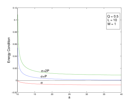
Figure 1: Variations of the expressions of energy conditions shown against a.

Using different values of mass $(M)$ and charge $(Q)$, we plot $\sigma$ and $p$ as a function of the a, shown in Figs.2-5.

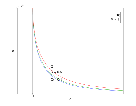
Figure 2: Plot for $\sigma$ versus a: Different values of charge(Q) when mass$(M=1)$ is fixed.

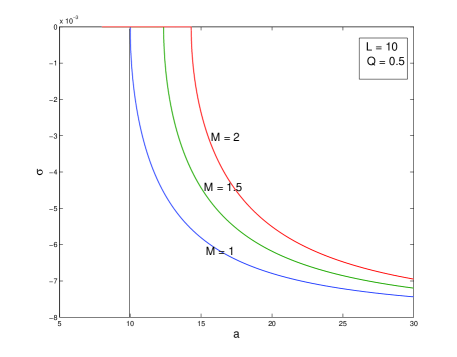
Figure 3: Plot for $\sigma$ versus a: Different values of mass$(M)$ when charge(Q=0.5) is fixed.

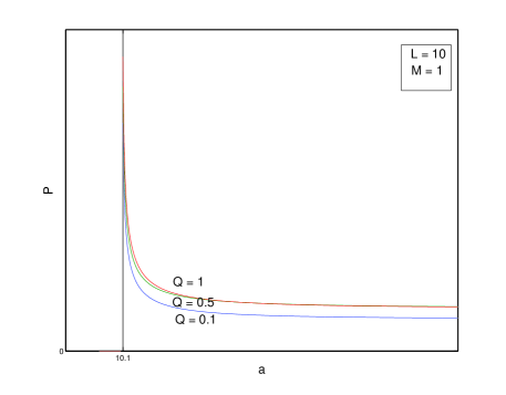
Figure 4: Plot for $p$ versus a: Different values of charge(Q) when mass$(M=1)$ is fixed.

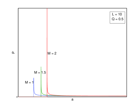
Figure 5: Plot for $p$ versus a: Different values of mass$(M)$ when charge(Q=0.5) is fixed.

III The gravitational field

In this section we analyze the attractive and repulsive nature of the wormhole, constructed from charged BTZ black hole and calculate the observer’s three-acceleration $a^{\mu}=u^{\mu}_{\,\,;\nu}u^{\nu}$, where $u^{\nu}=dx^{\nu}/d{\tau}=(1/\sqrt{f(r)},0,0)$. Only non-zero component for the line element in Eq.(1), is given by

$$a^{r}=\Gamma^{r}_{tt}\left(\frac{dt}{d\tau}\right)^{2}\\ =\frac{r}{L{{}^{2}}}-\frac{Q^{2}}{4r}.$$ (14)

A test particle when radially moving and initially at rest, obeys the equation of motion

$$\frac{d^{2}r}{d\tau^{2}}=-\Gamma^{r}_{tt}\left(\frac{dt}{d\tau}\right)^{2}=-a^{r},$$ (15)

which gives the geodesic equation if $a^{r}=0$. Also, we observe that the wormhole is attractive when $a^{r}>0$ and repulsive when $a^{r}<0$, which is shown in Fig.6

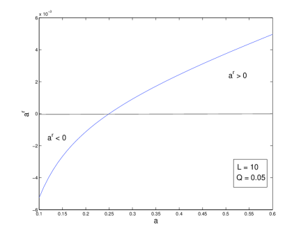
Figure 6: The wormhole is attractive when $a^{r}>0$ and repulsive when $a^{r}<0$.

IV The total amount of exotic matter

To construct such a thin-shell wormhole, we need exotic matter. Though, using BTZ in the thin-shell wormhole construction is that, it is not asymptotically flat and therefore the wormholes are not asymptotically flat. Recently Mazharimousavi, Halilsoy and Amirabi MH shown that a non-asymptotically flat black hole solution provides Stable thin-shell wormholes which are entirely supported by exotic matter.

In this section, we evaluate the total amount of exotic matter for the shell which can be quantified by the integral KY ; ES ; MC ; FK

$$\Omega_{\sigma}=\int[\rho+p_{r}]\sqrt{-g}d^{2}x,$$ (16)

where $g$ represents the determinant of the metric tensor. Now, by using the radial coordinate $R=r-a$, we have

$$\Omega_{\sigma}=\int^{2\pi}_{0}\int^{\infty}_{-\infty}[\rho+p_{r}]\sqrt{-g}\,dRd\phi.$$ (17)

For the infinitely thin shell it does not exert any radial pressure i.e. $p_{r}=0$ and using $\rho=\delta(R)\sigma(a)$ for above integral we have

$$\Omega_{\sigma}=\int^{2\pi}_{0}\left.[\rho\sqrt{-g}]\right|_{r=a}d\phi=2\pi a\sigma(a)\\ =-\frac{1}{2}\sqrt{\frac{a^{2}}{L{{}^{2}}}-\left[M+\frac{Q^{2}}{2}\ln(\frac{a}{L})\right]}.$$ (18)

With the help of graphical representation (Fig.7), we are trying to describe the variation of the total amount of exotic matter on the shell with respect to the mass and the charge.

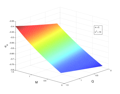
Figure 7: variation of the total amount of exotic matter on the shell with respect to the mass and the charge.

V Stability

Stability is one of the important issue for the wormhole. Here we analyze the stability of the shell from various angle.Our approaches are (i) phantom-like equation of state (ii)generalized chaplygin gas equation of state and (iii) linearized radial perturbation, around the static solution.

V.1 phantom-like equation of state

Here, we are trying to describe the stability of the shell considering the equation of state when the surface energy density and the surface pressure are taken into account. We set an equation $w=p/\sigma$ i.e. $p=w\sigma$ known as Phantom-like equation of state when $w<0$. Since, it is easy to check that the surface pressure and energy density obey the conservation equation

$$\frac{d(a\sigma)}{d\tau}+p\frac{d}{d\tau}(a)=0,$$ (19)

after differentiating w.r.t $\tau$, one can get

$$\frac{\dot{\sigma}}{\dot{a}}+\frac{1}{a}\left(\sigma+p\right)=0,$$ (20)

and using $p$=$w\sigma$, we get

$$\frac{d\sigma}{da}+\frac{1}{a}\sigma(1+w)=0.$$ (21)

Now, consider the static solution with radius $a=a_{0}$, we have

$$\sigma(a)=\sigma(a_{0})\left(\frac{a_{0}}{a}\right)^{(1+w)},$$ (22)

rearranging the Eq.(10) we can write

$$\dot{a}^{2}+V(a)=0.$$ (23)

Which is the equation of motion of the shell, where the potential V(a) is defined as

$$V(a)=f(a)-16\pi^{2}a^{2}\sigma^{2}(a).$$ (24)

Substitute the value of $\sigma(a)$ from Eq.(22), one can get

$$V(a)=\frac{a^{2}}{L{{}^{2}}}-\left[M+\frac{Q^{2}}{2}\ln(\frac{a}{L})\right]-16\pi^{2}a^{2}\sigma_{0}^{2}\left(\frac{a_{0}}{a}\right)^{2(1+w)},$$ (25)

where $\sigma_{0}=\sigma(a_{0})$, and rewriting the above equation we have

$$V(a)=\frac{a^{2}}{L{{}^{2}}}-\left[M+\frac{Q^{2}}{2}\ln(\frac{a}{L})\right]-16\pi^{2}a^{-2w}\mathcal{A}.$$ (26)

With $\mathcal{A}=\sigma^{2}_{0}a_{0}^{2(1+w)}$. Expanding $V(a)$ around the static solution i.e. at $a=a_{0}$, we have

$$V(a) = V(a_{0})+V^{\prime}(a_{0})(a-a_{0})+\frac{1}{2}V^{\prime\prime}(a_{0})(a-a_{0})^{2}$$ (27)

$$+O\left[(a-a_{0})^{3}\right],$$

where the primes denote the derivative with respect to a. The wormhole is stable if and only if $V(a_{0})$ has local minimum at $a_{0}$ and $V^{\prime\prime}(a_{0})>0$. Therefore, using the conditions $V(a_{0})=0$ and $V^{\prime}(a_{0})=0$, with $V^{\prime\prime}(a_{0})$ is given by

$$V^{\prime\prime}(a_{0})=\frac{2}{L{{}^{2}}}+\frac{Q^{2}}{2a^{2}_{0}}-32\pi^{2}\sigma^{2}_{0}w\left(2w+1\right).$$ (28)

We have verified that the inequality $V^{\prime\prime}(a_{0})>0$, holds for suitable choice of $Q$, $M$ and $L$ when $w$ takes the different values. We are trying to describe the stability of the configuration with help of graphical representation. In Figs.8-10, we plot the graphs to find the possible range of $a_{0}$ where $V(a_{0})$ possess a local minimum. Thus, fixing the values of $Q=0.5$, $M=1$ and $L=10$, we plot three different graphs (Figs.8-10), corresponding to the Eq.(28) for different values of $w=-0.1,-0.4,-2.5$ respectively, which represents different equation of state. In other words, we get stable thin-shell wormholes from charged BTZ black hole for different values of $w$.

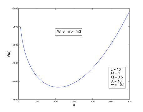
Figure 8: Stable wormhole when $w>-1/3$ i.e. when equation of quintessence state.

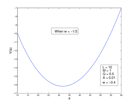
Figure 9: Stable wormhole when $w<-1/3$ i.e. when equation of dark energy state.

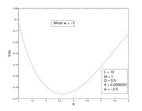
Figure 10: Stable wormhole when $w<-1$ i.e. when equation of phantom energy state.

V.2 Generalized Chaplygin gas equation of state

Here we are trying to check the stability of the shell considering Chaplygin gas equation of state, at the throat, which is a hypothetical substance satisfying an equation of state:

$$p=-\frac{A}{\sigma^{\alpha}},$$ (29)

where $\sigma$ is surface energy density and $p$ is surface pressure with $A$ positive constants and $0<\alpha\leq 1$.

substitute the values of $\sigma$ and $p$ (i.e. equations (10) and (11)) in equation (29), we get

$$\frac{(-1)^{\alpha}\left[\frac{a}{L{{}^{2}}}-\frac{Q^{2}}{4a}+\ddot{a}\right]}{(4\pi)^{\alpha+1}a^{\alpha}}\left[\frac{a^{2}}{L{{}^{2}}}-[M+\frac{Q^{2}}{2}\ln(\frac{a}{L})]+\dot{a}^{2}\right]^{\frac{\alpha-1}{2}}+A=0$$ (30)

For the case of static solution, the surface energy density and surface pressure are given by the equations (12) and (13), and relate to the equation(29), one can get the solution as

$$\frac{(-1)^{\alpha}}{(4\pi)^{\alpha+1}a^{\alpha}}\left[\frac{a}{L{{}^{2}}}-\frac{Q^{2}}{4a}\right]\left[\frac{a^{2}}{L{{}^{2}}}-[M+\frac{Q^{2}}{2}\ln(\frac{a}{L})]\right]^{\frac{\alpha-1}{2}}+A=0.$$ (31)

By assuming L.H.S of Eq.(31) as $\mathcal{G}(a)=0$, we get the throat radius of the shell at some $a=a_{0}$. In Fig(11), we show that $\mathcal{G}(a)$ cuts the a-axis at $a_{0}=2.8$ for the value of $\alpha=0.2$, which represents the radius of the throat of shell.

Now, we return to the conservation Eq.(20) and using Eq.(29), we have

$$\dot{\sigma}+\frac{\dot{a}}{a}\left(\frac{\sigma^{\alpha+1}-A}{\sigma^{\alpha}}\right)=0,$$ (32)

after solving the above equation, one can get

$$\sigma=\left[A+\left(\sigma_{0}^{\alpha+1}-A\right)\left(\frac{a_{0}}{a}\right)^{\alpha+1}\right]^{\frac{1}{\alpha+1}}.$$ (33)

where $\sigma_{0}$=$\sigma(a_{0})$. Therefore potential $V(a)$, as defined in Eq.(24) takes of the form

$$V(a)=f(a)-16\pi^{2}a^{2}\left[A+\left(\sigma_{0}^{\alpha+1}-A\right)\left(\frac{a_{0}}{a}\right)^{\alpha+1}\right]^{\frac{2}{\alpha+1}}.$$ (34)

Where

$$f(a)=\frac{a^{2}}{L{{}^{2}}}-\left[M+\frac{Q^{2}}{2}\ln(\frac{a}{L})\right].$$ (35)

The above solution gives a stable configuration if the second order derivative of the potential is positive for the static solution and $V(a_{0})$ posses a local minimum at $a_{0}$. To find the range of $a_{0}$ for which $V^{\prime\prime}(a_{0})>0$ we use graphical representation due to complexity of the expression $V^{\prime\prime}(a_{0})$ for the set of parameters in Eq.(34). Therefore, corresponding to the radius of the throat at $a_{0}=2.8$ (Fig.11), we are trying to find the possible range of $a_{0}$ for which $V(a_{0})$ posses a local minima. In Fig.12 we show the range of $a_{0}$ for the value of $\alpha=0.2$ and other corresponding parameters (values are given in the caption of the Fig. 12), for the stable configuration. Thus, we can get stable thin-shell wormholes supported by exotic matter filled with Chaplygin gas equation of state.

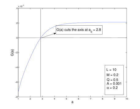
Figure 11: radius of the throat when $\mathcal{G}(a)=0$ cuts the axis a at some $a=a_{0}$.

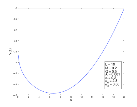
Figure 12: The stable wormhole for $0<\alpha\leq 1$ when $V(a)$ varies w.r.t a.

V.3 Linearized stability analysis

Now we are trying to find the stability of the configuration around the static solution at $a=a_{0}$ under radial perturbation. Applying the Taylor series expansion for the potential $V(a)$ around $a_{0}$, we get

$$V(a) = V(a_{0})+V^{\prime}(a_{0})(a-a_{0})+\frac{1}{2}V^{\prime\prime}(a_{0})(a-a_{0})^{2}$$ (36)

$$+O\left[(a-a_{0})^{3}\right],$$

where the prime denotes $d/da$. After differentiating Eq. (24), we obtain

$$V^{\prime}(a)=\frac{2a}{L{{}^{2}}}-\frac{Q^{2}}{2a}-32\pi^{2}a\sigma\left(\sigma+a\sigma^{\prime}\right).$$ (37)

Now from Eq.(20), we can write $\sigma^{\prime}$=$-\frac{1}{a}\left(\sigma+p\right)$ where $\sigma^{\prime}$=$\dot{\sigma}/\dot{a}$ and using Eq(37) we get

$$V^{\prime}(a)=\frac{2a}{L{{}^{2}}}-\frac{Q^{2}}{2a}+32\pi^{2}ap\sigma.$$ (38)

Again differentiating w.r.t a and using the parameter $\beta^{2}(\sigma)$ =$\left.\frac{\partial p}{\partial\sigma}\right|_{\sigma}$, one can get

$$V^{\prime\prime}(a)=\frac{2}{L{{}^{2}}}+\frac{Q^{2}}{2a^{2}}-32\pi^{2}p^{2}-32\pi^{2}\beta^{2}(p\sigma+\sigma^{2}).$$ (39)

Since we are linearizing around $a=a_{0}$, we require that $V(a_{0})=0$ and $V^{\prime}(a_{0})=0$. Now using the values of $\sigma$ and $p$ from Eqs.(12) and (13), we get the solution of $V^{\prime\prime}(a_{0})$ given by

$$V^{\prime\prime}(a_{0})=\frac{2}{L{{}^{2}}}+\frac{Q^{2}}{2a_{0}^{2}}-\frac{2\beta^{2}}{a_{0}^{2}}\left[\frac{Q^{2}}{4}-H\right]-2\frac{\left[\frac{a_{0}}{L{{}^{2}}}-\frac{Q^{2}}{4a_{0}}\right]^{2}}{\frac{a_{0}^{2}}{L{{}^{2}}}-H},$$ (40)

where $H=M+\frac{Q^{2}}{2}\ln(\frac{a_{0}}{L}).$

The configuration is in stable equilibrium if and only if $V^{\prime\prime}(a_{0})>0$. So starting with $V^{\prime\prime}(a_{0})=0$ and solve for $\beta^{2}$ we get

$${\beta_{0}}^{2}=\mathcal{X}_{0}(a_{0})\equiv 1+\frac{8a_{0}^{2}Q^{2}-\left(L{{}^{2}}Q^{4}+16H^{2}L{{}^{2}}\right)}{4a_{0}^{2}Q^{2}-4H\left(4a_{0}^{2}+L{{}^{2}}Q^{2}\right)+16H^{2}L{{}^{2}}}.$$ (41)

Here we observe that

$$(i)~{}~{}{\beta_{0}}^{2}<\mathcal{X}_{0}(a_{0}),~{}~{}if~{}~{}4a_{0}^{2}Q^{2}>L{{}^{2}}\left(Q^{4}+16H^{2}\right),$$

$$(ii)~{}~{}{\beta_{0}}^{2}>\mathcal{X}_{0}(a_{0}),~{}~{}if~{}~{}4a_{0}^{2}Q^{2}<L{{}^{2}}\left(Q^{4}+16H^{2}\right).$$

The value of ${\beta_{0}}^{2}$ which represent the velocity of sound for ordinary matter, does not exceed the speed of light and lies in the region of $0\leq{\beta_{0}}^{2}<1$. In Fig.13, the region of stability depicted below the solid line, corresponding to the values of $M=1$, $Q=0.5$, and $L^{2}=0.01$, where in Figs.(14-15), the region of stability depicted above the left and below the right of the solid line, corresponding to the value of $M=1$, $L^{2}=10$ and increasing the value of charge Q, respectively. In all cases the stability region of ${\beta_{0}}^{2}$ is grater than one. As we are dealing with exotic matter, we relaxed the range of ${\beta_{0}}^{2}$ for ordinary matter in our stability analysis for the thin-shell wormholes.

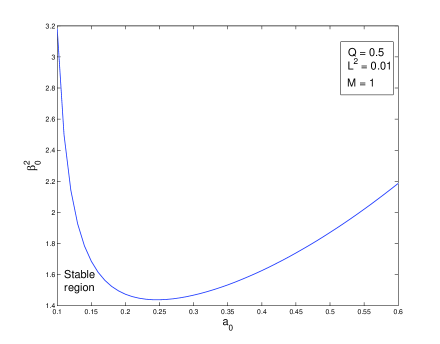
Figure 13: The region of stability is below the curve.

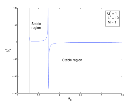
Figure 14: The region of stability is above the curve on the left and below the curve on the right.

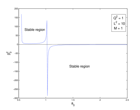
Figure 15: The region of stability is above the curve on the left and below the curve on the right .

VI Conclusions

In this work we construct charged thin-shell wormhole from BTZ black hole using the cut-paste technique. Though, a disadvantage with using BTZ in the thin-shell wormholes construction is that it is not asymptotically flat and therefore the wormholes are not asymptotically flat. Therefore, there is some ’matter’ at infinity. There is also ’matter due to the charge’. Vacuum solutions, or, at least asymptotically flat ones, are better because of the ’good’ behaviour at infinity.

We obtain the surface stress energy tensor at the junction by Lanczos equation where we observe that the energy density $\sigma$ is negative but pressure $p$ is positive. Also we get $\sigma+p$ and $\sigma+2p$ positive which shows matter contained by the shell violates the WEC but satisfy the NEC and SEC.

We draw our main attention on the stability of the shell considering different equation of state for the exotic matter at the throat. Firstly we consider dark, quintessence and phantom-like equation of state changing the value of $w$, where we found stable wormholes in all cases. Secondly we consider generalized Chaplygin gas equation of state and found stable wormhole for suitable choice of $\alpha$ with the help of graphical representation. Finally we studied the linearized stability analysis around the static solution i.e. at $a=a_{0}$ and we found stable wormholes in suitable range of $\beta^{2}_{0}$ with charged and mass though the behavior of $\beta_{0}$ is not clear to us for exotic matter.

Acknowledgments

AB is thankful to Dr. Farook Rahaman for this concept and helpful discussion.

References

- (1) M. Baados, C. Teitelboim, J. Zanelli: The Black Hole in Three Dimensional Space Time Phys. Rev. Lett. 69 (1992) 1849.
- (2) C. Martinez, C. Teitelboim and J. Zanelli. Phys. Rev.D61 (2000) 104013
- (3) M. S. Morris and K. S. Thorne: Wormholes in spacetime and their use for interstellar travel: A tool for teaching General Relativity Am. J. Phys. 56, 395 (1988).
- (4) D.Hochberg and M.Visser, Phys.Rev.D56,4745(1997).
- (5) Matt Visser,Sayan Kar and Naresh Dadhich: Traversable wormholes with arbitrarily small energy condition violations Phys.Rev.Lett.90:201102(2003).
- (6) J. P. S. Lemos, F. S. N. Lobo and S. Q. de Oliveira: Morris-Thorne wormholes with a cosmological constant Phys. Rev. D 68, 064004 (2003) [arXiv:gr-qc/0302049].
- (7) F. S. N. Lobo: Energy conditions, traversable wormholes and dust shells , Gen.Rel.Grav. 37 (2005) 2023-2038.
- (8) M. Visser: Lorentzian Wormholes: From Einstein to Hawking , (American Institute of Physics, New York, 1995).
- (9) Naresh Dadhich,Sayan Kar,Sailajananda Mukherji and Matt Visser: R = 0 space-times and selfdual Lorentzian wormholes , Phys.Rev.D65:064004(2002).
- (10) M. Visser, Nucl. Phys. B 328, 203 (1989).
- (11) Israel W 1966 Nuovo Cimento 44B 1
- (12) Papapetrou A and Hamoui A 1968 Ann. Inst. Henri Poincar e 9 179
- (13) Farook Rahaman,Saibal Ray,Abdul Kayum Jafry,Kausik Chakraborty: Singularity-free solutions for anisotropic charged fluids with Chaplygin equation of state Phys.Rev. D82 (2010) 104055.
- (14) Mubasher Jamil,Peter K.F. Kuhfittig,Farook Rahaman,Sk.A Rakib: Wormholes supported by polytropic phantom energy, Eur.Phys.J. C67 (2010) 513-520
- (15) Cecilia Bejarano: Ernesto F. Eiroa, Dilaton thin-shell wormholes supported by a generalized Chaplygin gas . Phys.Rev.D84:064043(2011).
- (16) Ernesto F. Eiroa: Thin-shell wormholes with a generalized Chaplygin gas . Phys.Rev.D80:044033(2009).
- (17) F. S. N. Lobo: Phantom energy traversable wormholes, Phys. Rev. D 71, 084011 (2005).
- (18) F. S. N. Lobo: Stable dark energy stars, Class. Quant. Grav. 23, 1525-1541 (2006).
- (19) M. C. Bento, O. Bertolami and A. A. Sen: Generalized Chaplygin Gas, Accelerated Expansion and Dark Energy-Matter Unification, Phys. Rev. D 66, 043507 (2002).
- (20) S. Sushkov: Wormholes supported by a phantom energy, Phys. Rev. D 71, 043520 (2005).
- (21) T. Multamaki, M. Manera and E. Gaztanaga: Large scale structure and the generalised Chaplygin gas as dark energy . Phys.Rev. D 69, 023004 (2004).
- (22) Peter K.F. Kuhfittig: The Stability of thin-shell wormholes with a phantom-like equation of state . Acta Phys.Polon.B41:2017-2019(2010).
- (23) E. Poisson and M. Visser: Thin-shell wormholes: Linearization stability . Phys. Rev. D 52, 7318 (1995).
- (24) F. S. N. Lobo and P. Crawford: Linearized stability analysis of thin-shell wormholes with a cosmological constant . Class. Quant. Grav. 21, 391 (2004).
- (25) E. Eiroa and C. Simeone Stability of charged thin shells :Rev. D83 (2011) 104009.
- (26) E. Eiroa and G. E. Romero: Linearized stability of charged thin shell wormholes . Rel.Grav. 36 (2004) 651-659.
- (27) A.A. Usmani, Z. Hasan , F. Rahaman, Sk.A. Rakib, Saibal Ray, Peter K.F. Kuhfittig: Thin-shell wormholes from charged black holes in generalized dilaton-axion gravity . Gen.Rel.Grav.42:2901-2912(2010).
- (28) F. Rahaman, K A Rahman, Sk.A Rakib, Peter K.F. Kuhfittig : Thin-shell wormholes from regular charged black holes . Int.J.Theor.Phys.49:2364-2378(2010).
- (29) Won Tae Kim,John J.Oh,Myung Seok Yo,Phys.Rev.D70:044006(2004).
- (30) Ji Young Han, Won Tae Kim, Hee Ju Yee ,Phys.Rev.D69:027501(2004). e-Print: arXiv:0707.0900 [gr-qc]
- (31) R. Sharma, F. Rahaman, I. Karar: A Class of interior solutions corresponding to a (2+1) dimensional asymptotically anti-de Sitter spacetime : Phys.Lett.B 704,1( 2011).
- (32) F. Rahaman, S. Ray, A. A. Usmani, S. Islam: The (2+1)-dimensional gravastars , arXiv:1108.4824[gr-qc].
- (33) Eduard Alexis Larranaga Rubio: Traversable wormholes construction in (2+1) gravity .
- (34) Farook Rahaman, A. Banerjee, I. Radinschi: A new class of stable (2+1) dimensional thin shell wormhole . Int.J.Theor.Phys. 51 (2012) 1680-1691.
- (35) M.S.R. Delgaty, Robert B,Mann: Traversable wormholes in (2+1)-dimensions and (3+1)-dimensions with a cosmological constant . Int.J.Mod.Phys. D4 (1995) 231-246
- (36) Robert B. Mann, John J. Oh Phys: Gravitationally Collapsing Shells in (2+1) Dimensions . Rev. D74 (2006) 124016
- (37) Misner C, Wheeler JA. Ann. of Phys. 1957; 2: 525-603.
- (38) Sung-Won Kim and Sang Pyo Kim : The Traversable wormhole with classical scalar fields . Phys.Rev. D58 (1998) 087703
- (39) Sung-Won Kim and Hyunjoo Lee : Exact solutions of a charged wormhole . Phys.Rev. D63 (2001) 064014
- (40) E. Babichev, V. Dokuchaev, Yu. : Eroshenko Black hole mass decreasing due to phantom energy accretion . Phys.Rev.Lett. 93 (2004) 021102
- (41) Mubasher Jamil, M. Akbar: Generalized second law of thermodynamics for a phantom energy accreting BTZ black hole . Gen.Rel.Grav. 43 (2011) 1061-1068.
- (42) Mazharimousavi, Halilsoy and Amirabi : d-dimensional non-asymptotically flat thin-shell wormholes in Einstein-Yang-Mills-Dilaton gravity Phys.Lett.A375:231-236(2011) .
- (43) Kamal Kanti Nandi, Yuan-Zhong Zhang, K.B. Vijaya Kumar: On volume integral theorem for exotic matter . Phys.Rev.D70:127503,2004.
- (44) Ernesto F. Eiroa , Claudio Simeone: Thin-shell wormholes in dilaton gravity . Phys.Rev. D71 (2005) 127501
- (45) Marc Thibeault, Claudio Simeone , Ernesto F. Eiroa: Thin-shell wormholes in Einstein-Maxwell theory with a Gauss-Bonnet term . Gen.Rel.Grav.38:1593-1608(2006).
- (46) F. Rahaman, M. Kalam,S. Chakraborty: Thin shell wormholes in higher dimensiaonal Einstein-Maxwell theory . Gen.Rel.Grav.38:1687-1695(2006).
- (47) Ernesto F. Eiroa: Claudio Simeone Cylindrical thin shell wormholes . Phys.Rev.D70:044008(2004).