Contextual Hypergraph Modelling for Salient Object Detection

Abstract

Salient object detection aims to locate objects that capture human attention within images. Previous approaches often pose this as a problem of image contrast analysis. In this work, we model an image as a hypergraph that utilizes a set of hyperedges to capture the contextual properties of image pixels or regions. As a result, the problem of salient object detection becomes one of finding salient vertices and hyperedges in the hypergraph. The main advantage of hypergraph modeling is that it takes into account each pixel’s (or region’s) affinity with its neighborhood as well as its separation from image background. Furthermore, we propose an alternative approach based on center-versus-surround contextual contrast analysis, which performs salient object detection by optimizing a cost-sensitive support vector machine (SVM) objective function. Experimental results on four challenging datasets demonstrate the effectiveness of the proposed approaches against the state-of-the-art approaches to salient object detection.

1 Introduction

Image saliency detection aims to effectively identify important and informative regions in images. Early approaches in this area focus mainly on predicting where humans look, and thus work only on human eye fixation data [1, 2, 3]. Recently, a large body of work concentrates on salient object detection [4, 5, 6, 7, 8, 9, 10, 11, 12, 13, 14, 15, 16, 17], whose goal is to discover the most salient and attention-grabbing object in an image. This has a wide range of applications such as image retargeting [18], image classification [19], and image segmentation [20, 21]. Because it is difficult to define saliency analytically, the performance of salient object detection is evaluated on datasets containing human-labeled bounding boxes or foreground masks.

Salient object detection is typically accomplished by image contrast computation, either on a local or a global scale. estimates the saliency degree of an image region by computing the contrast against its local neighborhood. Various contrast measures have been proposed, including mutual information [22], incremental coding length [3], and center-versus-surround feature discrepancy [6, 8, 9, 10, 13, 14, 15].

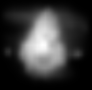
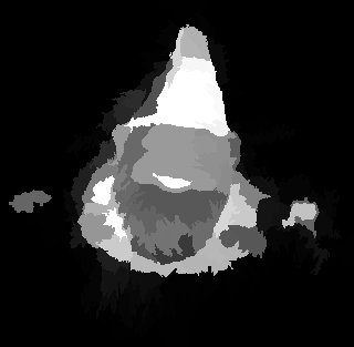
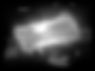
Image	SVM saliency	Hypergraph saliency

Figure 1: Illustration of our approaches to salient object detection.

Global salient object detection approaches [4, 5, 7, 11, 12] estimate the saliency of a particular image region by measuring its uniqueness in the entire image. These approaches model uniqueness by exploiting the global statistical properties of the image, including frequency spectrum analysis [4], color-spatial distribution modeling [7], high-dimensional Gaussian filtering [11], low-rank matrix decomposition [12], and geodesic distance computation [5].

Therefore, the definition of object saliency depends on the choice of context. Global saliency defines the context as the entire image, whereas local saliency requires the definition of a local context. In this work, we first show that within a fixed context, a cost-sensitive SVM can accurately measure saliency by capturing centre-surround contrast information. We then show that the use of a hypergraph captures more comprehensive contextual information, and therefore enhances the accuracy of salient object detection.

Here, we propose two approaches to salient object detection based on hypergraph modeling and imbalanced max-margin learning. Our main contributions are as follows.

1. We introduce hypergraph modeling into the process of image saliency detection for the first time. A hypergraph is a rich, structured image representation modeling pixels (or superpixels) by their contexts rather than their individual values. This additional structural information enables more accurate saliency measurement. The problem of saliency detection is naturally cast as that of detecting salient vertices and hyperedges in a hypergraph at multiple scales.

2. We formulate the centre-surround contrast approach to saliency as a cost-sensitive max-margin classification problem. Consequently, the saliency degree of an image region is measured by its associated normalized SVM coding length.

Example results of our approaches to salient object detection are shown in Fig. 1. We describe each approach in the following two sections, before evaluating them in Sec. 4.

2 Cost-sensitive SVM saliency detection

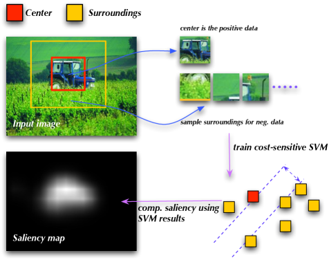
Figure 2: Illustration of cost-sensitive SVM for saliency detection. The saliency score is computed using Equ. (3) based on the SVM classification results.

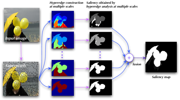
Figure 3: Illustration of hypergraph modeling for saliency detection using nonparametric clustering. The first column shows an input image and its associated over-segmented image with a set of superpixels. The middle columns display the multi-scale hyperedges (constructed by nonparametric clustering on the superpixels) and their corresponding results of hyperedge saliency evaluation. The rightmost image shows the final saliency map $HSa$ generated by multi-scale hyperedge saliency fusion. Note that the regions highlighted in different colors correspond to different hyperedges (i.e., superpixel cliques having some common visual properties). In theory, our hypergraph modeling can also work on pixels in a similar way.

As illustrated in [9, 23], saliency detection is typically posed as the problem of center-versus-surround contextual contrast analysis. To address this problem, we propose a saliency detection method based on imbalanced max-margin learning, which is capable of effectively discovering the local salient image regions that significantly differ from their surrounding image regions. In this case, the image is divided into overlapping rectangular windows which are tested for saliency. The context for each window is the windows that overlap it.

Before describing the method, we first introduce some notation used hereinafter. Let ${\bf x}_{1}$ denote the feature vector associated with a center image patch, and $\{{\bf x}_{\ell}\}_{\ell=2\dots N}$ denote the feature vectors associated with the spatial overlapping surrounding patches of the center image patch. Using these patches, the proposed method explores their inter-class separability in a max-margin classification framework.

As shown in the top-right part of Fig. 2, the center image patch ${\bf x}_{1}$ is thought of as a positive sample while the surrounding patches $\{{\bf x}_{\ell}\}_{\ell=2\dots N}$ are used as the negative samples. The saliency degree of ${\bf x}_{1}$ is determined by its inter-class separability from $\{{\bf x}_{\ell}\}_{\ell=2\dots N}$. In other words, if ${\bf x}_{1}$ could be easily separated from $\{{\bf x}_{\ell}\}_{\ell=2\dots N}$, then it is deemed to be salient; otherwise, its saliency degree is low. This is a binary classification problem, which is associated with a cost-sensitive classification objective function [24]:

$$\begin{array}[]{cc}\underset{{\bf w},b,{\boldsymbol{\epsilon}}}{\min}&J({\bf w},b,\boldsymbol{\epsilon})=\frac{1}{2}\|{\bf w}\|_{2}^{2}+\frac{1}{2}C\sum_{\ell=1}^{N}\nu_{\ell}\epsilon_{\ell}^{2},\\ \mbox{s.t.}&y_{\ell}=f({\bf x}_{\ell})+\epsilon_{\ell},\end{array}$$ (1)

where $\|\cdot\|_{2}$ is the $L_{2}$ norm, $f({\bf x})={\bf w}^{{\!\top}}{\bf x}+b$ is the classifier to learn; ${\boldsymbol{\epsilon}}$ is the residual vector; $C$ is the regularization parameter; and $\nu_{\ell}$ is the corresponding weight of ${\bf x}_{\ell}$ such that $\nu_{1}\gg\nu_{\ell}$ for $\ell=2\dots N$. We set all the negative samples to have the same weight $\nu_{\ell}$, $\ell=2\dots N$. According to the KKT condition, we have the following linear system:

$$\left[\begin{array}[]{cc}0&{\bf 1}^{{\!\top}}_{N}\\ {\bf 1}_{N}&\Omega+V_{C}\end{array}\right]\left[\begin{array}[]{c}b\\ {\boldsymbol{\alpha}}\end{array}\right]=\left[\begin{array}[]{c}0\\ {\bf y}\end{array}\right],$$ (2)

where ${\bf 1}_{N}\in\mathcal{R}^{N}$ is the all-one column vector, ${\bf y}=(y_{1},y_{2},\ldots,y_{N})^{{\!\top}}$ is the label vector, $\Omega=(\Omega_{ij})_{N\times N}$ is the kernel matrix $\Omega_{ij}={\bf x}_{i}^{{\!\top}}{\bf x}_{j}$, and $V_{C}$ is a diagonal matrix such that $V_{C}=\mbox{diag}(\frac{1}{C\nu_{1}},\frac{1}{C\nu_{2}},\ldots,\frac{1}{C\nu_{N}})$. Based on the solution $({\boldsymbol{\alpha}}^{\ast},b^{\ast})$ to the linear system (2), we have the weighted LS-SVM classifier $f({\bf x})=({\bf w}^{\ast})^{{\!\top}}{\bf x}+b^{\ast}$ with ${\bf w}^{\ast}=({\bf x}_{1},{\bf x}_{2},\ldots,{\bf x}_{N}){\boldsymbol{\alpha}}^{\ast}$.

Using the weighted LS-SVM classifier $f({\bf x})$, we define the saliency score as:

$$SSa({\bf x}_{1})=\frac{1}{N-1}\sum_{\ell=2}^{N}\frac{1-\mbox{sgn}(f({\bf x}_{\ell}))}{2},$$ (3)

where $\mbox{sgn}(\cdot)$ is a sign function and the term $\sum_{\ell=2}^{N}\frac{1-\mbox{sgn}(f({\bf x}_{\ell}))}{2}$ counts the number of correctly classified surrounding samples. Loosely speaking, the saliency score $SSa({\bf x}_{1})$ can be viewed as a normalized SVM coding length (i.e., training accuracy for the surrounding samples), which characterizes the inter-class separability between ${\bf x}_{1}$ and its surroundings $\{{\bf x}_{\ell}\}_{\ell=2\dots N}$. As shown in the bottom-left part of Fig. 2, the harder ${\bf x}_{1}$ is to separate from $\{{\bf x}_{\ell}\}_{\ell=2\dots N}$, the smaller $SSa({\bf x}_{1})$ will be. In other words, the center patch looks similar to its surroundings. Conversely, the larger $SSa({\bf x}_{1})$ indicates the lower similarity between ${\bf x}_{1}$ and $\{{\bf x}_{\ell}\}_{\ell=2\dots N}$, and hence a higher saliency degree. Note that, here the cost-sensitive LS-SVM is not the only choice. We can use other classifiers such as the exemplar SVM [25], where the standard hinge-loss SVM is used. We have used LS-SVM for its simplicity (it has a closed-form solution). Note that, this max-margin learning framework can be easily extended to perform saliency detection on a global scale. Namely, the image boundary patches can be treated as negative samples while the remaining image patches are used as positive samples. By running the max-margin learning procedure over such training samples, the saliency degree of each image patch can be measured by computing its distance to the separating hyperplane.

Example saliency maps derived from this measure are shown in Figs. 1 and 2. Although they accurately locate the salient object in each case, they also suffer from “fuzziness” or lack of precision around object boundaries and in locally homogeneous regions. This is mainly due to the center-surround local context that they are based on. In the next section, we describe an alternative approach based on segmentation based context that alleviates these problems.

Image	Hypergraph saliency	Standard graph saliency

Figure 4: Illustration of salient object detection using two different types of graphs (i.e., hypergraph and standard pairwise graph). Clearly, our hypergraph saliency measure is able to accurately capture the intrinsic structural properties of the salient object.

3 Hypergraph modeling for saliency detection

To more effectively find salient object regions, we propose a hypergraph modeling based saliency detection method that forms contexts of superpixels to capture both internal consistency and external separation. Fig. 3 shows the high-level flowchart of the proposed method.

As illustrated in [26], a hypergraph is a graph comprising a set of vertices and hyperedges. In contrast to the pairwise edge in a standard graph, the hyperedge in a hypergraph is a high-order edge associated with a vertex clique linking more than two vertices. Effectively constructing such hyperedges is crucial for encoding the intrinsic contextual information on the vertices in the hypergraph.

Hypergraph modeling

In our method, an image $I$ is modeled by a hypergraph $\mathcal{G}=(\mathcal{V},\mathcal{E})$, where $\mathcal{V}=\{v_{i}\}$ is the vertex set corresponding to the image superpixels and $\mathcal{E}=\{e_{j}\}$ is the hyperedge set comprising a family of subsets of $\mathcal{V}$ such that $\bigcup_{e\in\mathcal{E}}=\mathcal{V}$ [26]. As shown in Fig. 3, these hyperedges are constructed by multi-scale clustering, which groups the image superpixels into a set of superpixel cliques. Each clique corresponds to a collection of superpixels having some common visual properties, and works as a hyperedge of the hypergraph $\mathcal{G}$. The process of hyperedge construction implicitly encodes intrinsic affinity information on superpixels. Namely, if two superpixels have a higher co-occurrence frequency in the hyperedges, they tend to share more visual properties and have a higher visual similarity.

A hyperedge can also be viewed as a high-order context that enforces the contextual constraints on each superpixels in the hyperedge. As a result, the saliency of each superpixel, as measured by the hyperedges it belongs to, is not only determined by the superpixel itself but also influenced by its associated contexts. Due to such contextual constraints on each superpixel, we simply convert the original saliency detection problem to that of detecting salient vertices and hyperedges in the hypergraph $\mathcal{G}$. Mathematically, the hypergraph $\mathcal{G}$ is associated with a $|\mathcal{V}|\times|\mathcal{E}|$ incidence matrix ${\bf H}=(H(v_{i},e_{j}))_{|\mathcal{V}|\times|\mathcal{E}|}$:

$$H(v_{i},e_{j})=\left\{\begin{array}[]{ll}1,&\mbox{if}\thickspace v_{i}\in e_{j},\\ 0,&\mbox{otherwise}.\end{array}\right.$$ (4)

The saliency value of any vertex $v_{i}$ in $\mathcal{G}$ is defined as:

$$HSa(v_{i})=\sum_{e\in\mathcal{E}}\Gamma(e)H(v_{i},e),$$ (5)

where $\Gamma(e)$ encodes the saliency information on the hyperedge $e$. In essence, our hypergraph saliency measure (5) is a generalization of the standard pairwise saliency measure defined as:

$$PSa(v_{i})=\sum_{v_{j}\in\mathcal{N}_{v_{i}}}d_{(v_{i},v_{j})}=\sum_{e\in\{(v_{i},v_{j})|j\neq i\}}\mathbb{I}_{e}d_{e}H(v_{i},e),$$ (6)

where $\mathcal{N}_{v_{i}}$ stands for the neighborhood of $v_{i}$, $d_{(v_{i},v_{j})}$ measures the saliency degree of the pairwise edge $(v_{i},v_{j})$, and $\mathbb{I}_{e}$ is the pairwise adjacency indicator (s.t. $\mathbb{I}_{e}=1$ if $v_{j}\in\mathcal{N}_{v_{i}}$; otherwise, $\mathbb{I}_{e}=0$). Instead of using simple pairwise edges, our hypergraph saliency measure takes advantage of the higher-order hyperedges (i.e., superpixel cliques) to effectively capture the intrinsic structural properties of the salient object, as shown in Fig. 4. To implement this approach, we need to address the following two key issues: 1) how to adaptively construct the hyperedge set $\mathcal{E}$; and 2) how to accurately measure the saliency degree $\Gamma(e)$ of each hyperedge.

Adaptive hyperedge construction

A hyperedge in the hypergraph $\mathcal{G}$ is actually a superpixel clique whose elements have some common visual properties. To capture the hierarchial visual saliency information, we construct a set of hyperedges by adaptively grouping the superpixels according to their visual similarities at multiple scales. In theory, this can be carried out in many ways using any number of established segmentation and clustering techniques.

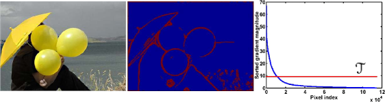
Figure 5: Illustration of the gradient magnitude information for hyperedge saliency evaluation. The left subfigure shows the original image, and the middle subfigure displays the gradient magnitude map $I_{g}^{\ast}$ obtained by binarizing $I_{g}$ using the adaptive threshold $\mathcal{T}$, as illustrated in the right subfigure.

Non-parametric clustering is typically associated with a kernel density estimator:

$$\widehat{f}_{k}({\bf p})=\frac{C_{k}}{Q|{\boldsymbol{\Sigma}}|^{\frac{1}{2}}}\sum_{i=1}^{Q}k(M^{2}({\bf p},{\bf p}_{i},{\boldsymbol{\Sigma}})),$$ (7)

where ${\bf p}_{i}$ is a feature vector associated with the $i$-th superpixel (generated from image oversegmentation), $k(\cdot)$ is a kernel profile ($k(x)=\exp(-x/2)$ in our case), ${\boldsymbol{\Sigma}}$ is a symmetric positive definite bandwidth matrix (in the experiments, ${\boldsymbol{\Sigma}}=\gamma^{2}{\bf I}$ with $\gamma$ being a scaling factor and ${\bf I}$ being an identity matrix), $M^{2}({\bf p},{\bf p}_{i},{\boldsymbol{\Sigma}})=({\bf p}-{\bf p}_{i})^{{\!\top}}{\boldsymbol{\Sigma}}^{-1}({\bf p}-{\bf p}_{i})$ stands for the Mahalanobis distance, and $C_{k}$ is a normalization constant. Therefore, the superpixel cliques can be discovered by seeking the modes of $\widehat{f}_{k}({\bf p})$. Mathematically, the mode-seeking problem can be converted to that of locating the zeros of the gradient $\nabla\widehat{f}_{k}({\bf p})=0$, which leads to the following iterative procedure:

$${\bf p}^{t+1}=\frac{\sum_{i=1}^{Q}g(M^{2}({\bf p}^{t},{\bf p}_{i},{\boldsymbol{\Sigma}})){\bf p}_{i}}{\sum_{i=1}^{Q}g(M^{2}({\bf p}^{t},{\bf p}_{i},{\boldsymbol{\Sigma}}))},$$ (8)

where $g(x)=-k^{\prime}(x)$ and the superscript $t$ indexes the iteration number. To accelerate the optimization process (8), we adopt a fast agglomerative mean-shift clustering method based on iterative query set compression [27].

Each mode is associated with a hyperedge, containing all the superpixels that converge to it after running the iterative procedure (8). The bandwidth matrix ${\boldsymbol{\Sigma}}=\gamma^{2}{\bf I}$ controls the scaling properties of the hyperedge. Consequently, using different values of $\gamma$ for nonparametric clustering can generate the hyperedges at different scales, as shown in Fig. 3. By using different configurations of $\gamma$, we obtain a set of multi-scale hyperedges $\{e_{i}\}$ with $e_{i}$ being the $i$-th hyperedge.

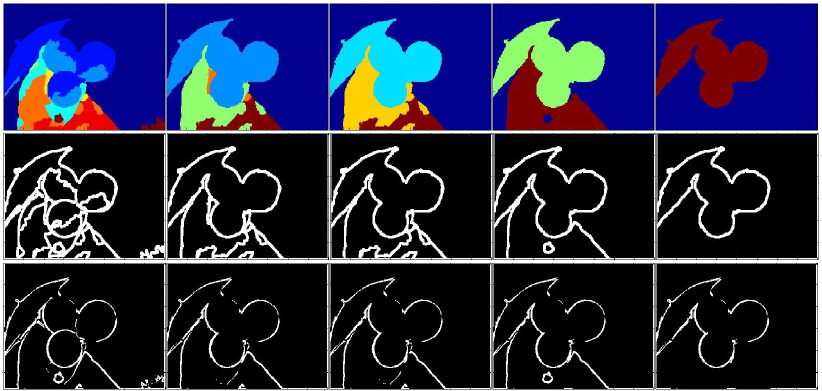
Figure 6: Illustration of $M_{g}$ and $I_{g}^{\ast}\circ M_{g}$ for hyperedge saliency evaluation. The top row shows the multi-scale hyperedges; the middle row displays the scale-specific $M_{g}$ that indicates the pixels (within a narrow band) along the boundary of the scale-specific hyperedge; and the bottom row exhibits the filtered gradient magnitude map $I_{g}^{\ast}\circ M_{g}$.

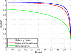
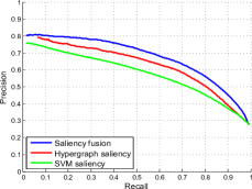
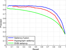
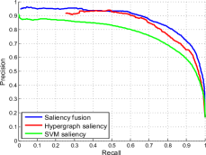
Figure 7: PR curves based on three different configurations: 1) using the SVM saliency approach only; and 2) using the hypergraph saliency approach only; 3) combining the SVM and hypergraph saliency approaches. Clearly, the saliency detection performance of using the third configuration outperform that of using the first and second configurations. From left to right: MSRA-1000, SOD, SED-100, and Imgsal-50.

Hyperedge saliency evaluation

By construction, a hyperedge defines a group of pixels that is internally consistent. In addition, a salient hyperedge should have the following two properties: 1) it should be enclosed by strong image edges; and 2) its intersection with the image boundaries ought to be small [5, 13]. Therefore, we measure the saliency degree of a scale-specific hyperedge $e$ by summing up the corresponding gradient magnitudes of the pixels (within a narrow band) along the boundary of the hyperedge. If the hyperedge touches the image boundaries, we decrease its saliency degree by a penalty factor.

More specifically, edge detection (using the Sobel operator in our case) is carried out for image $I$. Let $I_{x}$ and $I_{y}$ denote the x-axis and y-axis gradient magnitude maps, respectively. Thus, the final gradient magnitude map $I_{g}$ has the following entry: $I_{g}(m,n)=\sqrt{I_{x}^{2}(m,n)+I_{y}^{2}(m,n)}$. To obtain a robust gradient map, we introduce the following criterion: $I_{g}^{\ast}(m,n)=1$ if $I_{g}(m,n)>\mathcal{T}$; otherwise, $I_{g}^{\ast}(m,n)=0$, as shown in Fig. 5. Here, $\mathcal{T}$ is a threshold (picking out the top 10% of the $I_{g}$’s elements in our case). As a result, the saliency value of the hyperedge $e$ is computed as:

$$\Gamma(e)=\omega_{e}\left[\|I_{g}^{\ast}\circ M_{g}(e)\|_{1}-\rho(e)\right].$$ (9)

Here, $\omega_{e}$ is a scale-specific hyperedge weight (a larger scale leads to a larger weight), $\|\cdot\|_{1}$ is the 1-norm, $M_{g}(e)$ is a binary mask (illustrated in Fig. 6) indicating the pixels (within a narrow band) along the boundary of the hyperedge $e$, $\circ$ is the elementwise dot product operator, and $\rho(e)$ is a penalty factor that is equal to the number of the image boundary pixels shared by the hyperedge $e$. Based on Equ. (5), we obtain the hypergraph saliency measure $HSa(v_{i})$ for any vertex $v_{i}$ in the hypergraph $\mathcal{G}$.

After both SVM and hypergraph saliency detection, we obtain the corresponding saliency maps. Each element of these saliency maps is mapped into [0, 255] by linear normalization, leading to the normalized saliency maps. Finally, the final saliency map is obtained by linearly combining the SVM and hypergraph saliency detection results.

4 Experiments

4.1 Experimental setup

Datasets

As a subset of the MSRA dataset [8], MSRA-1000 [4] is a commonly used benchmark dataset for salient object detection. SOD [28] is composed of 300 challenging images. SED-100 is a subset of the SED dataset [29, 30], and consists of 100 images. Each image in SED-100 contains only one salient object. Imgsal-50 is a subset of the Imgsal dataset [31], and comprises 50 images with large salient objects for evaluation. Each image in the aforementioned datasets contains a human-labelled foreground mask used as ground truth for salient object detection.

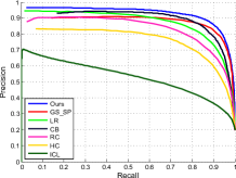
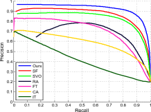
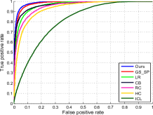
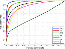
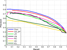
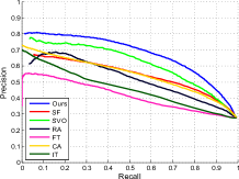
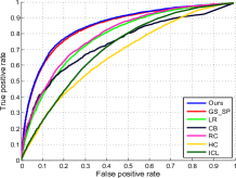
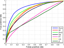
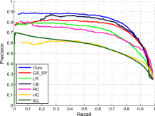
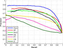
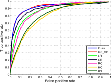
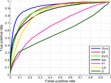
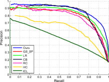
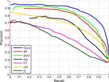
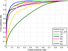
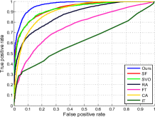
Figure 8: Quantitative PR and ROC performance of all the thirteen approaches on the four datasets. The left two columns show the PR curves while the right two columns display the ROC curves. The rows from top to bottom correspond to MSRA-1000, SOD, SED-100, and Imgsal-50, respectively. Clearly, our approach achieve a better PR and ROC performance than the other competing approaches in most cases.

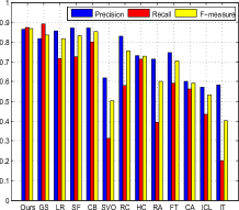
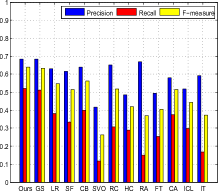
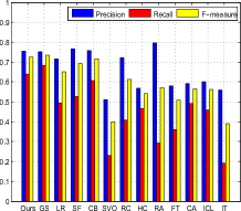
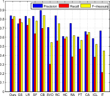
Figure 9: Quantitative F-measure performance of all the thirteen approaches on the four datasets. The columns from left to right correspond to MSRA-1000, SOD, SED-100, and Imgsal-50, respectively. Here, GS is a shorthand form of GS_SP. It is clear that our approach achieve a good F-measure performance on the four datasets.

Evaluation criterion

For a given saliency map, we adopt four criteria to evaluate the quantitative performance of different approaches: precision-recall (PR) curves, F-measures, receiver operating characteristic (ROC) curves, and VOC overlap scores. Specifically, the PR curve is obtained by binarizing the saliency map using a number of thresholds ranging from 0 to 255, as in [4, 7, 12, 11]. As described in [4], F-measure is computed as $F=((\beta^{2}+1)P\cdot R)/(\beta^{2}P+R)$. Here, $P$ and $R$ are the precision and recall rates obtained by binarizing the saliency map using an adaptive threshold that is twice the overall mean saliency value [4]. $\beta^{2}=0.3$ is the same as that in [4]. Identical to [30], the ROC curve is generated from true positive rates and false positive rates obtained during the calculation of the corresponding PR curve. The VOC Overlap score [32] is defined as $\frac{|S\cap S^{\prime}|}{|S\cup S^{\prime}|}$. Here, $S$ is the ground-truth foreground mask, and $S^{\prime}$ is the object segmentation mask obtained by binarizing the saliency map using the same adaptive threshold during the calculation of F-measure.

Image	GT	Ours	GS SP[5]	LR[12]	SF[11]	CB[13]	SVO[15]	RC[7]	HC[7]	RA[16]	FT[4]	CA[14]	ICL[3]	IT[1]

Figure 10: Salient object detection examples of all the thirteen approaches on the four datasets: MSRA-1000 (rows 1-3), SOD (rows 4-6), SED-100 (row 7), and Imgsal-50 (row 8). It is clear that our approach obtains the visually more consistent saliency detection results than the other competing approaches.

	Ours	GS SP [5]	LR [12]	SF [11]	CB [13]	SVO [15]	RC [7]	HC [7]	RA [16]	FT [4]	CA [14]	ICL [3]	IT [1]
MSRA-1000	0.77$\pm$0.20	0.75$\pm$0.22	0.63$\pm$0.25	0.67$\pm$0.24	0.72$\pm$0.24	0.29$\pm$0.24	0.52$\pm$0.31	0.59$\pm$0.29	0.37$\pm$0.33	0.50$\pm$0.27	0.40$\pm$0.19	0.33$\pm$0.19	0.17$\pm$0.12
SOD	0.40$\pm$0.22	0.38$\pm$0.20	0.29$\pm$0.19	0.27$\pm$0.20	0.31$\pm$0.25	0.11$\pm$0.19	0.24$\pm$0.23	0.22$\pm$0.20	0.14$\pm$0.17	0.19$\pm$0.17	0.27$\pm$0.19	0.22$\pm$0.17	0.14$\pm$0.11
SED-100	0.52$\pm$0.25	0.56$\pm$0.27	0.41$\pm$0.27	0.47$\pm$0.27	0.52$\pm$0.32	0.21$\pm$0.29	0.34$\pm$0.31	0.37$\pm$0.30	0.27$\pm$0.28	0.30$\pm$0.26	0.35$\pm$0.32	0.34$\pm$0.22	0.16$\pm$0.14
Imgsal-50	0.69$\pm$0.18	0.65$\pm$0.21	0.64$\pm$0.18	0.59$\pm$0.22	0.64$\pm$0.19	0.29$\pm$0.29	0.52$\pm$0.25	0.45$\pm$0.27	0.37$\pm$0.30	0.37$\pm$0.19	0.47$\pm$0.19	0.30$\pm$0.21	0.19$\pm$0.10

Table 1: Quantitative performance of all the thirteen approaches in VOC overlap scores on the four datasets. Clearly, our approach obtains the highest VOC overlap score with a low variance in most cases.

Implementation details

In the experiments, cost-sensitive SVM saliency detection on an image is performed at different scales, each of which corresponds to a scale-specific image patch size for center-versus-surround contrast analysis. The final SVM saliency map is obtained by averaging the multi-scale saliency detection results. For computational efficiency, we first choose a fixed-sized image $8\times 8$ patch and then resize the image using different downsampling rates to simulate the scale changes. In addition, each image patch is represented as a vectorized RGB feature vector. During the optimization process (1), the weight $\nu_{1}$ for the center image patch is chosen as 0.5 while the weights $\nu_{k}$ (s.t. $k>1$) for the surrounding image patches are set to 0.01, as suggested in [25]. Each superpixel ${\bf p}_{i}$ (referred to Equ. (8)) is first generated from image over-segmentation, and then represented by an 8-dimensional feature vector, which is obtained by averaging the corresponding color vectors of all the pixels in the superpixel. The color vector for each pixel contains four normalized color components ${\bf c}=(l,a,b,h)$ and their associated elementwise power transforms [33] from the LAB and HSV color spaces. In the experiments, the final saliency detection results are further refined by graph-based manifold propagation. We did not carefully tune the aforementioned parameters in the experiments. Note that the aforementioned parameters are fixed throughout all the experiments.

4.2 Evaluation of our individual approaches

Here, we evaluate the saliency detection performance of the proposed approaches based on three different configurations: 1) using the SVM saliency approach only; 2) using the hypergraph saliency approach only; and 3) combining the SVM and hypergraph saliency approaches. Fig. 7 shows their quantitative results of salient object detection in the aspect of PR curves. From Fig. 7, it is clearly seen that the saliency detection performance of only using the SVM saliency approach is significantly enhanced after combining the hypergraph saliency approach. The reason is that the hypergraph saliency approach captures both the internal consistency and strong boundary properties of salient objects. By incorporating the SVM saliency approach, the saliency detection results of only using the hypergraph saliency approach are further smoothed, leading to an improved saliency detection accuracy. Therefore, we use the best configuration (i.e., combination of SVM and hypergraph saliency) for performance evaluations in the following experiments.

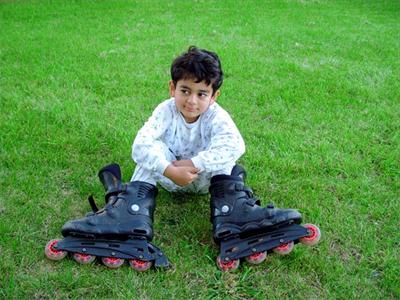
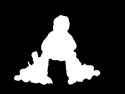
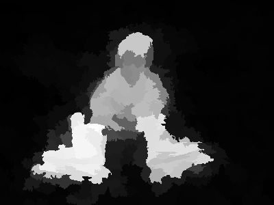
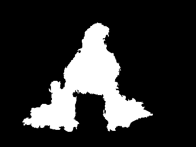
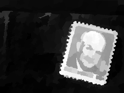
Figure 11: Examples of salient object segmentation. From left to right: input images, ground truth, saliency maps, segmentation results. Clearly, our approach obtains visually consistent segmentation results with ground truth.

4.3 Comparison of saliency detection approaches

In the experiments, we qualitatively and quantitatively compare the proposed approach with twelve state-of-the-art approaches, including GS SP [5], LR [12], SF [11], CB [13], SVO [15], RC [7], HC [7], RA [16], FT [4], CA [14], ICL [3], and IT [1]. These approaches are implemented using their either publicly available source code or original saliency detection results from the authors.

Fig. 8 shows the quantitative saliency detection performance of the proposed approach against the twelve competing approaches in the PR and ROC curves on the four datasets. From the left half of Fig. 8, we see that the proposed approach achieves the highest precision rate in most cases when the recall rate is fixed. Given a fixed false positive rate, the proposed approach obtains a higher true positive rate than the other approaches in most cases, as shown in the right half of Fig. 8.

From Fig. 9, it is observed that the proposed approach achieves the best F-measure performance on the two popular benchmark datasets, that is, MSRA-1000 and SOD. On the SED-100 dataset, GS SP and the proposed approach obtain the best results, and the F-measure of the proposed approach is slightly lower than GS SP. On the Imgsal-50 dataset, the proposed approach is one of the two best approaches, and achieves a slightly lower F-measure than CB. In addition, Fig. 10 shows several salient object detection examples of all the thirteen approaches. It is seen from Fig. 10 that our approach obtain visually more feasible saliency detection results than the other competing approaches.

Furthermore, Tab. 1 shows the corresponding VOC overlap scores of all the thirteen approaches. It is seen from Tab. 1 that the proposed approach obtains the highest VOC overlap score with a low variance in most cases. Besides, Fig. 11 gives three intuitive examples of salient object segmentation (i.e., binarization using the adaptive threshold [4]) based on the proposed approach. From Fig. 11, we observe that the proposed approach achieves the visually consistent segmentation results with ground truth.

Figure 12: Qualitative image retargeting performance comparison between [18] and ours. From left to right: images, our results, results of [18]. Clearly, the performance of our approach is better than that of [18].

4.4 Application to image retargeting

The goal of image retargeting is to reduce image size while preserving important content. As shown in [18], saliency detection plays an important role in image retargeting. Following the work of [18], we directly replace its saliency detection component with ours while keeping the other components fixed. Fig. 12 shows some image retargeting examples of the two approaches (i.e., [18] and ours) on the image retargeting dataset from [18]. Clearly, our approach obtains more visually feasible results. This indicates that our approach is capable of effectively preserving the intrinsic structural information on salient objects during image retargeting.

5 Conclusion

In this work, we have proposed two salient object detection approaches based on hypergraph modeling and center-versus-surround max-margin learning. Specifically, we have designed a hypergraph modeling approach that captures the intrinsic contextual saliency information on image pixels/superpixels by detecting salient vertices and hyperedges in a hypergraph. Furthermore, we have developed a local salient object detection approach based on center-versus-surround max-margin learning, which solves an imbalanced cost-sensitive SVM optimization problem. Compared with the twelve state-of-the-art approaches, we have empirically shown that the fusion of our approaches is able to achieve more accurate and robust results of salient object detection.

Acknowledgments This work is in part supported by ARC grants LP120200485 and FT120100969. Correspondence should be addressed to C. Shen.

References

- [1] L. Itti, C. Koch, and E. Niebur. A model of saliency-based visual attention for rapid scene analysis. IEEE Trans. Pattern Anal. Mach. Intell., 20(11):1254–1259, 1998.
- [2] N. Bruce and J. Tsotsos. Saliency based on information maximization. In Proc. Adv. Neural Inf. Process. Syst., 2005.
- [3] X. Hou and L. Zhang. Dynamic visual attention: searching for coding length increments. In Proc. Adv. Neural Inf. Process. Syst., pages 681–688, 2008.
- [4] R. Achanta, S. Hemami, F. Estrada, and S. Susstrunk. Frequency-tuned salient region detection. In Proc. IEEE Conf. Comp. Vis. Patt. Recogn., pages 1597–1604, 2009.
- [5] Y. Wei, F. Wen, W. Zhu, and J. Sun. Geodesic saliency using background priors. In Proc. Eur. Conf. Comp. Vis., pages 29–42, 2012.
- [6] J. Feng, Y. Wei, L. Tao, C. Zhang, and J. Sun. Salient object detection by composition. In Proc. IEEE Int. Conf. Comp. Vis., pages 1028–1035, 2011.
- [7] M. Cheng, G. Zhang, N. Mitra, X. Huang, and S. Hu. Global contrast based salient region detection. In Proc. IEEE Conf. Comp. Vis. Patt. Recogn., pages 409–416, 2011.
- [8] T. Liu, J. Sun, N. Zheng, X. Tang, and H. Shum. Learning to detect a salient object. In Proc. IEEE Conf. Comp. Vis. Patt. Recogn., 2007.
- [9] D. Klein and S. Frintrop. Center-surround divergence of feature statistics for salient object detection. In Proc. IEEE Int. Conf. Comp. Vis., pages 2214–2219, 2011.
- [10] B. Alexe, T. Deselaers, and V. Ferrari. What is an object? In Proc. IEEE Conf. Comp. Vis. Patt. Recogn., pages 73–80, 2010.
- [11] F. Perazzi, P. Krahenbuhl, Y. Pritch, and A. Hornung. Saliency filters: Contrast based filtering for salient region detection. In Proc. IEEE Conf. Comp. Vis. Patt. Recogn., pages 733–740, 2012.
- [12] X. Shen and Y. Wu. A unified approach to salient object detection via low rank matrix recovery. In Proc. IEEE Conf. Comp. Vis. Patt. Recogn., pages 853–860, 2012.
- [13] H. Jiang, J. Wang, Z. Yuan, T. Liu, N. Zheng, and S. Li. Automatic salient object segmentation based on context and shape prior. In Proc. Brit. Mach. Vis. Conf., 2011.
- [14] S. Goferman, L. Zelnik-Manor, and A. Tal. Context-aware saliency detection. In Proc. IEEE Conf. Comp. Vis. Patt. Recogn., pages 2376–2383, 2010.
- [15] K. Chang, T. Liu, H. Chen, and S. Lai. Fusing generic objectness and visual saliency for salient object detection. In Proc. IEEE Int. Conf. Comp. Vis., pages 914–921, 2011.
- [16] E. Rahtu, J. Kannala, M. Salo, and J. Heikkilä. Segmenting salient objects from images and videos. In Proc. Eur. Conf. Comp. Vis., pages 366–379, 2010.
- [17] C. Yang, L. Zhang, H. Lu, X. Ruan, and M.-H. Yang. Saliency detection via graph-based manifold ranking. In Proc. IEEE Conf. Comp. Vis. Patt. Recogn., pages 3166–3173, 2013.
- [18] J. Sun and H. Ling. Scale and object aware image retargeting for thumbnail browsing. In Proc. IEEE Int. Conf. Comp. Vis., pages 1511–1518, 2011.
- [19] G. Sharma, F. Jurie, and C. Schmid. Discriminative spatial saliency for image classification. In Proc. IEEE Conf. Comp. Vis. Patt. Recogn., pages 3506–3513, 2012.
- [20] L. Wang, J. Xue, N. Zheng, and G. Hua. Automatic salient object extraction with contextual cue. In Proc. IEEE Int. Conf. Comp. Vis., pages 105–112, 2011.
- [21] Y. Lu, W. Zhang, H. Lu, and X. Xue. Salient object detection using concavity context. In Proc. IEEE Int. Conf. Comp. Vis., pages 233–240, 2011.
- [22] D. Gao, V. Mahadevan, and N. Vasconcelos. The discriminant center-surround hypothesis for bottom-up saliency. In Proc. Adv. Neural Inf. Process. Syst., 2007.
- [23] D. H. Hubel and T. N. Wiesel. Receptive fields and functional architecture in two nonstriate visual areas. J. Neurophysiology, 28:229–289, 1965.
- [24] J. A. K. Suykens, J. De Brabanter, L. Lukas, and J. Vandewalle. Weighted least squares support vector machines: robustness and sparse approximation. Neurocomputing, 48(1):85–105, 2002.
- [25] T. Malisiewicz, A. Gupta, and A. Efros. Ensemble of exemplar-svms for object detection and beyond. In Proc. IEEE Int. Conf. Comp. Vis., pages 89–96, 2011.
- [26] D. Zhou, J. Huang, and B. Scholköpf. Learning with hypergraphs: Clustering, classification, and embedding. In Proc. Adv. Neural Inf. Process. Syst., 2007.
- [27] X. Yuan, B. Hu, and R. He. Agglomerative mean-shift clustering. IEEE Trans. on Knowledge and Data Engineering, 24(2):209–219, 2012.
- [28] V. Movahedi and J. Elder. Design and perceptual validation of performance measures for salient object segmentation. In Proc. IEEE Conf. Comp. Vis. Patt. Recogn. Workshops, pages 49–56, 2010.
- [29] S. Alpert, M. Galun, R. Basri, and A. Brandt. Image segmentation by probabilistic bottom-up aggregation and cue integration. In Proc. IEEE Conf. Comp. Vis. Patt. Recogn., pages 1–8, 2007.
- [30] A. Borji, D. Sihite, and L. Itti. Salient object detection: A benchmark. In Proc. Eur. Conf. Comp. Vis., pages 414–429, 2012.
- [31] J. Li, M. Levine, X. An, X. Xu, and H. He. Visual saliency based on scale-space analysis in the frequency domain. IEEE Trans. Pattern Anal. Mach. Intell., 35:996–1010, 2013.
- [32] A. Rosenfeld and D. Weinshall. Extracting foreground masks towards object recognition. In Proc. IEEE Int. Conf. Comp. Vis., pages 1371–1378, 2011.
- [33] X. Ren and L. Bo. Discriminatively trained sparse code gradients for contour detection. In Proc. Adv. Neural Inf. Process. Syst., pages 593–601, 2012.