Probing the metallicity and ionization state of the circumgalactic medium at $z\sim 6$ and beyond with OI absorption

Abstract

Low ionization metal absorption due to O i has been identified as an important probe of the physical state of the inter-/circumgalactic medium at the tail-end of reionization. We use here high-resolution hydrodynamic simulations to interpret the incidence rate of O i absorbers at $z\sim 6$ as observed by Becker et al. (2011). We infer weak O i absorbers (EW $\ga$ 0.1 Å) to have typical H i column densities in the range of sub-DLAs, densities of 80 times the mean baryonic density and metallicities of about 1/500 th solar. This is similar to the metallicity inferred at similar overdensities at $z\sim 3$, suggesting that the metal enrichment of the circumgalactic medium around low-mass galaxies has already progressed considerably by $z\sim 6$. The apparently rapid evolution of the incidence rates for O i absorption over the redshift range $5\lesssim z\lesssim 6$ mirrors that of self-shielded Lyman-Limit systems at lower redshift and is mainly due to the rapid decrease of the meta-galactic photo-ionization rate at $z\ga 5$. We predict the incidence rate of O i absorbers to continue to rise rapidly with increasing redshift as the IGM becomes more neutral. If the distribution of metals extends to lower density regions, O i absorbers will allow the metal enrichment of the increasingly neutral filamentary structures of the cosmic web to be probed.

1 Introduction

Lyman-$\alpha$ absorption line studies are an important tool to study the ionization state of the IGM at the tail-end of reionization (e.g. Songaila 2004; Fan et al. 2006; Bolton & Haehnelt 2007; Becker, Rauch & Sargent 2007; McQuinn et al. 2008; Mesinger 2010; Becker & Bolton 2013). At $z>6$, however, little detailed information can be obtained from Lyman-$\alpha$ absorption about the spatial distribution of the neutral gas, as a significant fraction of the IGM is opaque to Lyman series photons. As pointed out by Oh (2002), O i absorption provides an interesting alternative to study the distribution of neutral metal enriched gas in the IGM. O i has an atomic transition with a rest wavelength longer than Ly$\alpha$, so is visible redward of the Ly$\alpha$ emission. O i also has an ionization energy close to that of neutral hydrogen ($\Delta E=0.019\,\mathrm{eV}$) and is an excellent tracer of (self-shielded) neutral gas.

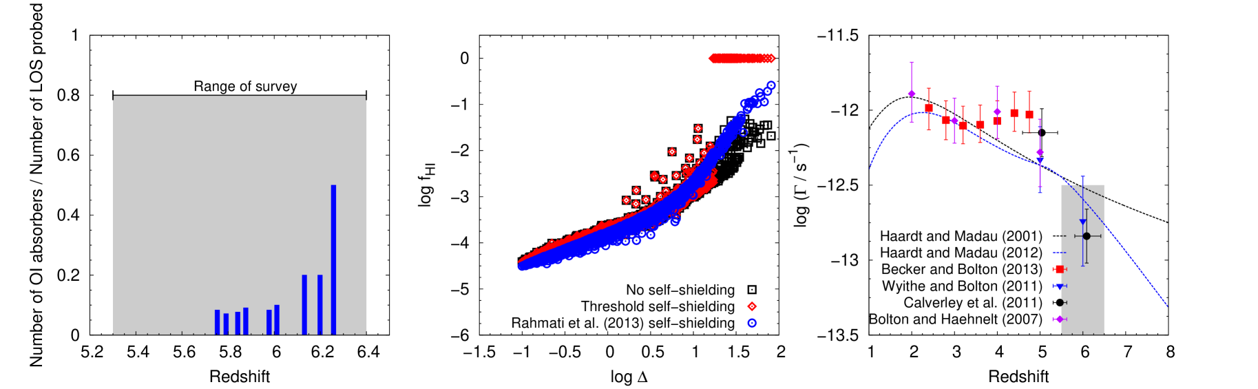
Figure 1: Left: The incidence rate of O i absorbers in the survey of Becker et al. (2011). Nine systems containing O i were detected. The height of the bars is the ratio of the number of O i absorbers to the number of sightlines that were surveyed at the redshift of the absorber. All of the O i absorption systems were found at $z>5.75$ and the line of sight number density of absorbers appears to increase rapidly with increasing redshift. Middle: The dependence of neutral fraction on overdensity for the simulation with no self-shielding, with the threshold self-shielding model used in Bolton & Haehnelt (2013) and the self-shielding prescription used in Rahmati et al. (2013a). The photo-ionization rate in this case was taken to be $\log(\Gamma/\textnormal{s}^{-1})=-12.8$. Right: A plot of the background photo-ionization rate $\Gamma$ against redshift $z$. The points are measurements of the UV background at different redshifts taken from Becker & Bolton (2013), Wyithe & Bolton (2011), Calverley et al. (2011) and Bolton & Haehnelt (2007). The Haardt & Madau (2001) and Haardt & Madau (2012) models for $\Gamma$ are also shown. The shaded grey region shows the range of $\Gamma$ consistent with the observed incidence rate of O i absorbers at $z\sim 6$.

The most comprehensive searches for O i absorption at high redshift so far have been performed by Becker, Rauch & Sargent (2007) and Becker et al. (2011). The results of the Becker et al. (2011) survey are summarised in the left panel of Figure 1 and Table 1. The survey was based on spectra of 17 QSOs with emission redshifts ranging from $5.8<z_{\textnormal{\scriptsize{em}}}<6.4$. High-resolution spectra were obtained for nine of the QSOs, using Keck (HIRES) or Magellan (MIKE) and moderate-resolution spectra were obtained for the rest using Keck (ESI). Ten low-ionization metal systems were detected, with nine of these systems containing O i lines. The O i absorption systems are summarised in Table 1. The total absorption path-length of the 2011 survey was $\Delta X=39.5$, where $X$ is defined as

$$X(z)=\int^{z}_{0}\,\frac{H_{0}}{H(z^{\prime})}(1+z^{\prime})^{2}\,\mathrm{d}z^{\prime},$$ (1)

and $H(z)$ is the Hubble constant at redshift $z$ (Bahcall & Peebles, 1969).

Even though the survey path extends from $z=5.3$, all ten detected systems occur at $z>5.75$ and, as the left panel of Figure 1 demonstrates, the incidence of low-ionization systems appears to increase rapidly with increasing redshift. Becker et al. (2011) suggested that this rapid evolution is due to the evolution of the meta-galactic UV background at $z\sim 6$. They further pointed out that the overall incidence rate is comparable to that of Damped Lyman-$\alpha$ systems (DLAs) and Lyman-Limit systems (LLSs) at $z\sim 3$ and proposed that the absorbers may be probing the circumgalactic medium of faint galaxies at high redshift (see Kulkarni et al. (2013) and Maio, Ciardi & Müller (2013) for recent modelling of DLA host galaxies and metal enrichment at these high redshifts).

Table 1: Equivalent width of the O i lines observed by Becker et al. (2011)

QSO	$z_{\textnormal{\scriptsize{abs}}}$	Instrument	$W_{\lambda}$ (Å)
SDSS J2054-0005	5.9776	ESI	0.124
SDSS J2315-0023	5.7529	ESI	0.238
SDSS J0818+1722	5.7911	HIRES	0.182
SDSS J0818+1722	5.8765	HIRES	0.058
SDSS J1623+3112	5.8415	HIRES	0.391
SDSS J1148+5251	6.0115	HIRES	0.162
SDSS J1148+5251	6.1312	HIRES	0.079
SDSS J1148+5251	6.1988	HIRES	0.020
SDSS J1148+5251	6.2575	HIRES	0.036

There are still many questions to be answered, however, about the spatial distribution of the gas giving rise to this absorption and the physical properties of the absorbing gas, as well as the link between these absorbers and self-shielded absorption systems at lower redshift. While the incidence rate of DLAs appears to evolve rather slowly with redshift (e.g. Seyffert et al. 2013), the incidence rate of LLSs is increasing rapidly with increasing redshift (Fumagalli et al., 2013; Songaila & Cowie, 2010). Bolton & Haehnelt (2013, BH13) have recently emphasized that this rapid evolution of LLSs is expected to accelerate further as the tail-end of the epoch of reionization is probed.

In this paper, we will use the same hydrodynamical simulation used in BH13 to reproduce the observed damping wing redward of the Lyman-$\alpha$ emission in the $z=7.085$ QSO ULASJ1120+0641 (Mortlock et al., 2011) to model the O i absorbers of Becker et al. (2011). The simulations have been shown to reproduce well the properties of the Lyman-$\alpha$ forest in QSO absorption spectra over a wide redshift range $2\la z\la 6$ and should allow us to obtain a reasonable representation of the spatial distribution of neutral self-shielded gas at $z\geq 6$, where the meta-galactic photo-ionization rate is expected to drop rapidly. To model the O i absorption, we adopt a relatively simple approach, where we assume a simple power-law metallicity-density relation and apply self-shielding corrections to our simulations, which do not include radiative transfer. This allows us to vary the metal distribution and ionization state sufficiently to obtain a good match for the data and to constrain in this way both the metal/oxygen distribution and the ionization state of the CGM/IGM. Recently Finlator et al. (2013) have attempted to model the distribution of metals and self-shielded gas from first principles with full radiative transfer simulations. This approach, based on much more expensive ab initio simulations, is offering important complementary insights towards a self-consistent picture for the production and transport of metals and ionizing photons.

We will discuss the details of our simulations in section 2. Section 3 will describe our modelling of the O i absorbers in the Becker et al. (2011) survey. In section 4, we will discuss our results with regard to metallicity and photo-ionization rate of the inter-/circumgalactic medium and present predictions for the evolution of O i absorption at $z>6$. Section 5 gives a summary and our conclusions. A calculation of the neutral fraction of O i with the photo-ionization code CLOUDY (Ferland et al., 1998) is presented in an appendix.

2 Modelling the high-redshift IGM

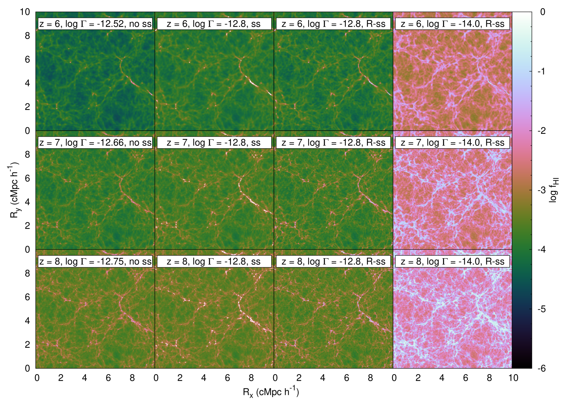
Figure 2: The neutral hydrogen fraction of the simulation. The top row is at $z=6.0$, the middle row is at $z=7.1$ and the bottom row is at $z=8.0$. Shown is a thin slice of thickness $39h^{-1}\,\mathrm{ckpc}$ midway through the simulation box with boxsize $10h^{-1}\,\mathrm{cMpc}$. From left: column 1 does not include self-shielding, column 2 shows the threshold self-shielding model used in Bolton & Haehnelt (2013) with $\log(\Gamma/\textnormal{s}^{-1})=-12.8$, column 3 includes self-shielding using the Rahmati et al. (2013a) model with $\log(\Gamma/\textnormal{s}^{-1})=-12.8$, and column 4 includes self-shielding using the Rahmati et al. (2013a) model with $\log(\Gamma/\textnormal{s}^{-1})=-14.0$.

2.1 Hydrodynamical simulation of the CGM and IGM

Our modelling is based on a cosmological hydrodynamical simulation with outputs at redshifts $z=(6.0,7.1,8.0)$. The simulation, described in detail in BH13, was performed using the parallel TreeSPH code gadget-3 (the previous version of the code, gadget-2, is described in Springel (2005)). The simulation has a gas particle mass of $9.2\times 10^{4}h^{-1}\,\text{M}_{\odot}$ and a box of size $10h^{-1}\,\text{cMpc}$ (where cMpc refers to comoving Mpc). The gravitational softening length was $0.65h^{-1}\,\text{ckpc}$. The following values were assumed for the cosmological parameters $(h,\Omega_{\text{m}},\Omega_{\Lambda},\Omega_{\text{b}}\,h^{2},\sigma_{8},n)=(0.72,0.26,0.74,0.023,0.80,0.96)$.

In the simulation, the IGM is reionized instantaneously by a uniform photo-ionizing background at $z=9$. The photo-ionizing background is based on the Haardt & Madau (2001) model for emission from quasars and galaxies. The simulation does not include radiative transfer and was performed assuming the optically thin limit for ionizing radiation. The left column of panels in Figure 2 show the neutral fraction for a thin slice of the simulation midway through the simulation box in the optically thin limit. The hydrogen photo ionization rates $\Gamma$ are those of the Haardt & Madau (2001) model as indicated on the plot. The neutral fraction of the gas increases with increasing redshift, as expected. No fully neutral regions (shaded white) are seen in these optically thin simulations. Regions surrounded by neutral hydrogen column densities with $\log N_{\textnormal{\scriptsize{HI}}}\ga 17$ are, however, optically thick for ionizing radiation and the gas self-shields. This is neglected in the optically thin approximation. We model this by post-processing the simulations with simple models for the self-shielding as described in the next section.

2.2 Modelling self-shielded regions

We used two methods to add self-shielded regions to our simulation in post-processing. The first method approximates the effect of self-shielding by assuming a simple density threshold above which the gas becomes fully neutral (Haehnelt, Steinmetz & Rauch, 1998). This is motivated by numerical simulations of the IGM, which show that the gas responsible for the intervening Lyman-$\alpha$ absorption exhibits a reasonably tight correlation between (absorption-weighted) density and the column density of the absorbers. As in BH13 we first applied a simple self-shielding model that assumes that the absorption length corresponds to the Jeans length of gas in photo-ionization equilibrium as proposed by Schaye (2001).

The assumed density threshold is given by

$$\Delta_{\textnormal{\scriptsize{ss}}}=36\,\Gamma^{2/3}_{-12}\,T^{2/15}_{4}\,\left(\frac{\mu}{0.61}\right)^{1/3}\,\left(\frac{f_{\textnormal{\scriptsize{e}}}}{1.08}\right)^{-2/3}\,\left(\frac{1+z}{8}\right)^{-3}.$$ (2)

Here, $\Delta=\rho\,/\,\overline{\rho}$ is the overdensity, $\Gamma_{-12}=\Gamma/10^{-12}\,\textnormal{s}^{-1}$ is the background photo-ionization rate and $T_{4}=T/10^{4}\,\textnormal{K}$, with $T$ the temperature of the gas. As already mentioned, this approximation assumes the typical size of an absorber to be the local Jeans length. It also assumes that the column density at which a LLS becomes self-shielding is $\log N_{\mathrm{HI}}=17.2$. Note that the case-A recombination coefficient for ionized hydrogen was used as given in Abel et al. (1997).

Rahmati et al. (2013a) have recently demonstrated that the above threshold self-shielding model, while being a reasonable first-order approximation, corresponds to a significantly sharper transition than predicted by full radiative transfer simulations that take recombination radiation into account. We therefore also implemented a simple fitting formulae suggested by Rahmati et al. (2013a) based on their simulations that include radiative transfer. In the Rahmati et al. (2013a) self-shielding model, the photo-ionization rate is assumed to be a smooth function of the density which can be approximated as,

$$\begin{split}\frac{\Gamma_{\textnormal{\scriptsize{Phot}}}}{\Gamma_{\textnormal{\scriptsize{HI}}}}=\,0.98&\,\bigg{[}1+\bigg{(}\frac{n_{\textnormal{\scriptsize{H}}}}{n_{\textnormal{\scriptsize{H,ss}}}}\bigg{)}^{1.64}\bigg{]}^{-2.28}\\ +\,&0.02\,\bigg{[}1+\frac{n_{\textnormal{\scriptsize{H}}}}{n_{\textnormal{\scriptsize{H,ss}}}}\bigg{]}^{-0.84}.\end{split}$$ (3)

$\Gamma_{\textnormal{\scriptsize{Phot}}}$ is the total photo-ionization rate and $n_{\textnormal{\scriptsize{H,ss}}}$ is the characteristic number density for self-shielding, which can be related to $\Delta_{\textnormal{\scriptsize{ss}}}$. The neutral fraction of the gas can then be calculated using $\Gamma_{\textnormal{\scriptsize{Phot}}}$, $n_{\textnormal{\scriptsize{H}}}$ and the temperature of the gas.

A comparison of the neutral fraction as a function of overdensity for the simple threshold self-shielding model, the Rahmati et al. (2013a) model and the case of no self-shielding is shown in the middle panel of Figure 1 for our simulations at $z=6$ with $\log(\Gamma/\textnormal{s}^{-1})=-12.8$ (our fiducial value consistent with Lyman-$\alpha$ forest measurements at $z\sim 6$ based on both the effective optical depth and the proximity effect method shown in the right panel). In the case of no self-shielding, the gas in the simulation is highly ionized everywhere. Even at the highest overdensities, the neutral fraction of the gas is still only about one percent. The Rahmati et al. (2013a) model predicts a neutral fraction close to that of our optically thin simulation at low overdensities ($\Delta\lesssim 1$), but the transition to fully neutral gas is much more gentle than in the threshold self-shielding model. At intermediate overdensities corresponding to sub-DLA column densities, the predicted neutral fraction changes smoothly from 1 percent for LLS column densities to 100 percent for DLA column densities. As we will see later, the significant difference in the predicted neutral fraction for sub-DLA column densities for the two self-shielding models is important for our estimates of the metallicity [O/H] of the observed O i absorbers.

In the second to fourth panels of Figure 2, we show the effect of the two self-shielding models on the distribution of neutral hydrogen. The threshold self-shielding model is only shown for our fiducial value $\log(\Gamma/\textnormal{s}^{-1})=-12.8$. The Rahmati et al. (2013a) self-shielding model was applied to the simulation for two different assumed values of the photo-ionization rate, $\log(\Gamma/\textnormal{s}^{-1})=-12.8$ and $\log(\Gamma/\textnormal{s}^{-1})=-14.0$, respectively.

As $\Gamma$ decreases, the density threshold for self-shielding decreases and the fully neutral self-shielded regions fill an increasing fraction of the volume in the simulations. The self-shielded regions “move out” from the outer part of galaxy haloes into the filaments (Miralda-Escudé, Haehnelt & Rees, 2000). As discussed by BH13, the increase of the volume filling factor of self-shielded regions directly translates into an increase of the expected incidence rate of H i absorbers optically thick to ionizing radiation. As we will see later this can also explain nicely why Becker et al. (2011) observed an increasing incidence of O i systems with increasing redshift. Note that, over this redshift interval, the incidence of self-shielded regions may be impacted far more strongly by changes in the photo-ionization rate than by the evolution of the density field.

3 Comparing simulated and observed O I absorbers

3.1 Synthetic O I absorption spectra

Using sightlines extracted from the simulation, synthetic O i spectra were generated by first calculating the optical depth and hence the normalised flux. The optical depth at each pixel was calculated using the temperature of the gas, its peculiar velocity, the number density of H i and assuming a relationship $n_{\textnormal{\scriptsize{OI}}}=Z_{\rm O}\,f_{\textnormal{\scriptsize{OI}}/\textnormal{\scriptsize{HI}}}\,n_{\textnormal{\scriptsize{HI}}}$. Here, $Z_{\rm O}$ is the metallicity of the gas which is applied to the simulation in post-processing and $f_{\textnormal{\scriptsize{OI}}/\textnormal{\scriptsize{HI}}}$ is the ratio of the neutral fractions of O i and H i which we estimated using the photo-ionization code CLOUDY (Ferland et al., 1998) as described in the appendix. The solar abundance of oxygen was taken as $\log Z_{\rm O,\odot}=-3.13$ (Asplund et al., 2009). The effect of instrumental broadening was included by convolving the spectra with a Gaussian with a FWHM of 6.7 km s^-1, equal to the instrumental profile of HIRES (which accounts for the majority of the O i detections in the Becker et al. (2011) sample.)

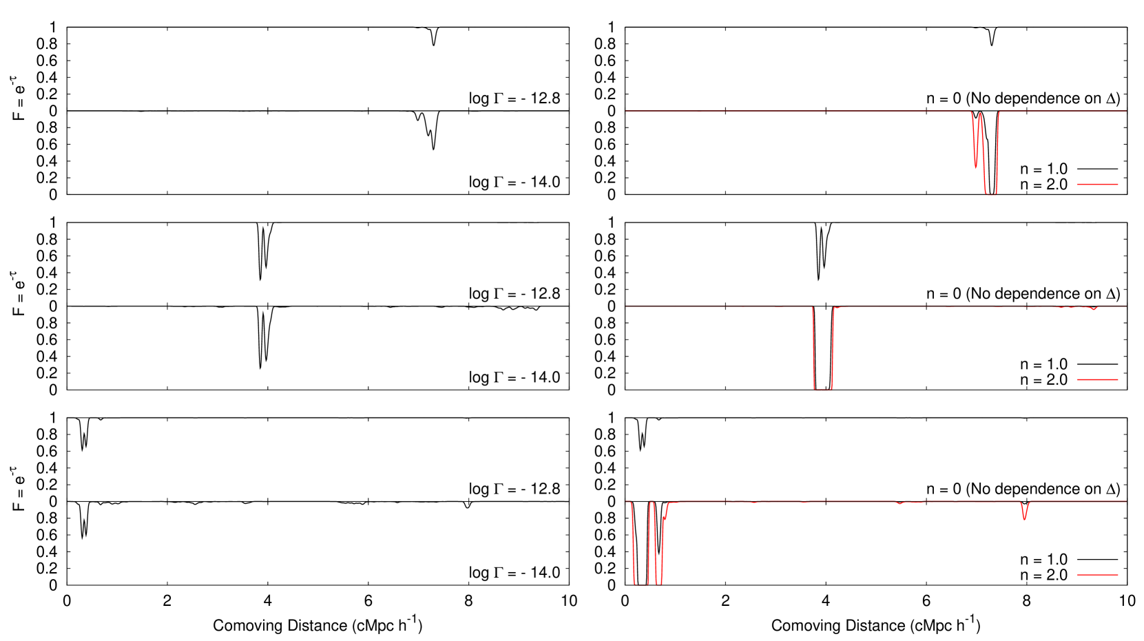
Figure 3: Left: Comparison of simulated O i spectra for two different background photo-ionization rates for three different sightlines through the simulation at $z=6.0$. The Rahmati et al. (2013a) self-shielding model was used. The top spectrum has $\log(\Gamma/\textnormal{s}^{-1})=-12.8$ and the bottom spectrum has $\log(\Gamma/\textnormal{s}^{-1})=-14.0$. The metallicity is $Z=10^{-2}\,Z_{\odot}$. Right: Comparison of simulated O i spectra for different values of the power law index $n$ of the metallicity model. The Rahmati et al. (2013a) self-shielding model was used with background photo-ionization rate $\log(\Gamma/\textnormal{s}^{-1})=-12.8$.

The left panel of Figure 3 shows the effect of changing $\Gamma$ on the O i spectra for three different sightlines. The spectra were generated assuming $\log(\Gamma/\textnormal{s}^{-1})=(-12.8,-14.0)$. As expected, there are more absorption lines in the spectra simulated assuming a smaller $\Gamma$, due to the increasing volume filling factor of fully neutral regions seen in Figure 2.

3.2 Modelling the metallicity as a function of overdensity

To model the O i absorption, we also need to make assumption for the metallicity [O/H] of the absorbing gas. To do this from first principles is difficult as this requires correctly modelling where and how efficiently stars form, as well as the metal yields and the transport and mixing of metals out of the galaxies into the circumgalactic and intergalactic media (see Finlator et al. (2013) for a recent attempt with regard to O i absorption). The density range probed by the absorbers is rather limited and we will make here the simple assumption of a power-law dependence of the metallicity, $Z\propto\Delta^{n}$, without any scatter. This is certainly a rough approximation but, as we will see later, it allows us to reproduce the O i absorbers remarkably well. We normalize this power-law model at an overdensity in the middle of the range probed by the simulated O i absorbers.

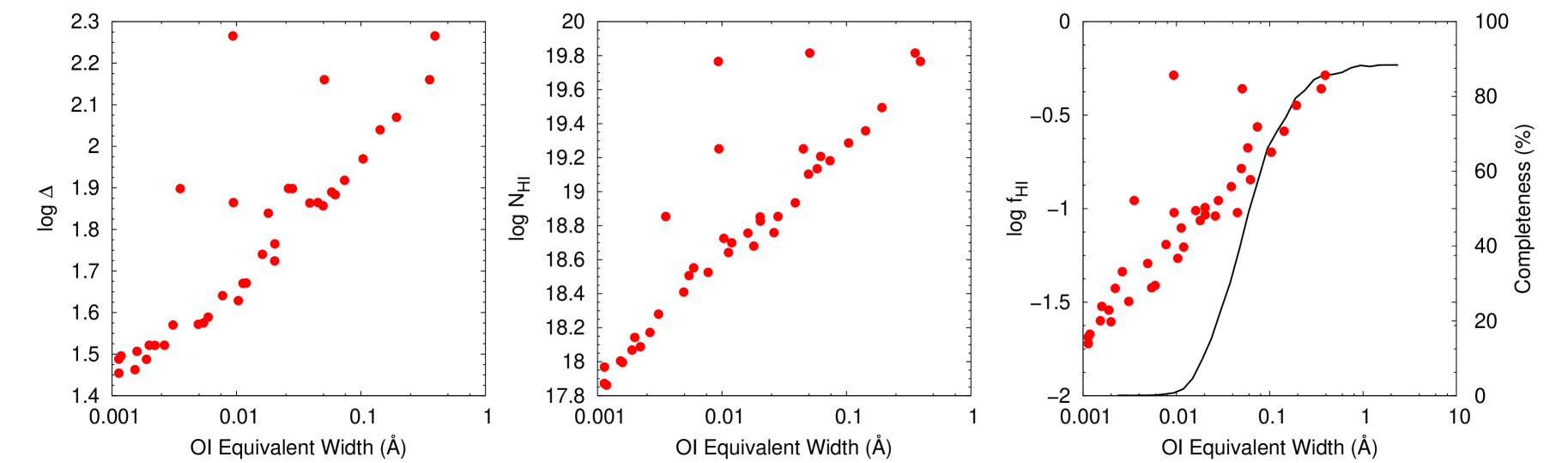
Figure 4: Left: The maximum overdensity probed by simulated O i absorbers as a function of their equivalent width for a model that reproduces the incidence rate observed by Becker et al. (2011) at $z=6.0$. The Rahmati et al. (2013a) model for self-shielding was used in each of the three panels. Middle: The H i column density of simulated O i absorbers as a function of their equivalent width. Right: The circles are the neutral hydrogen fraction of simulated O i absorbers as a function of their equivalent width. An estimate of the completeness of the observed sample of O i absorbers by Becker et al. (2011) as a function of their equivalent width is shown as the black curve with values on the right hand side axis of the panel. The completeness estimate does not reach 100 per cent as some regions of the quasar absorption spectra are contaminated due to atmospheric absorption or lines from other atomic transitions.

The left panel of Figure 4 shows the range of overdensities probed by the simulated O i absorbers for a model that fits the incidence rate observed by Becker et al. (2011). The overdensities probed range from $1.4<\log\Delta<2.3$ at $z=6.0$. An overdensity $\Delta=80$ falls approximately in the middle of this range and was used as pivot point for the power-law model of the metallicity. The metallicity was thus parameterized as,

$$Z=Z_{80}\,\left(\frac{\Delta}{80}\right)^{n},$$ (4)

where $Z_{80}$ is the metallicity at $\Delta=80$ and $n$ is the power-law index. The right panel of Figure 3 shows the effect on the O i spectra of varying this power-law index for $n=(0,1,2)$.

The H i column densities probed by the simulated O i absorbers are shown in the middle panel of Figure 4. They range from $17.8<\log N_{\textnormal{\scriptsize{HI}}}<19.9$. As we will discuss in more detail in the appendix O i is a good tracer of H i if the gas is “well-shielded”. The right panel of Figure 4 shows the neutral hydrogen fraction of the O i absorbers, which ranges from 10 percent to fully neutral for absorbers with EW $>0.01\,\mathrm{\AA}$.

3.3 Comparison to observations

To compare the simulated O i absorption to the Becker et al. (2011) sample, the equivalent widths (EWs) of the lines were measured. A threshold flux was calculated and regions where the calculated flux was lower than this threshold were identified as absorption features. The equivalent width per pixel was then calculated and summed over the number of pixels spanned by the absorption feature to calculate the total equivalent width.

Becker et al. (2011) have quantified the effect of noise on the detection probability of their O i absorbers, so the equivalent widths were measured for synthetic spectra with no added noise. An estimate of the completeness of the sample as a function of equivalent width as determined by Becker et al. (2011) for their observed sample is shown as the solid curve in the right panel of Figure 4 (with values on the right hand side axis).

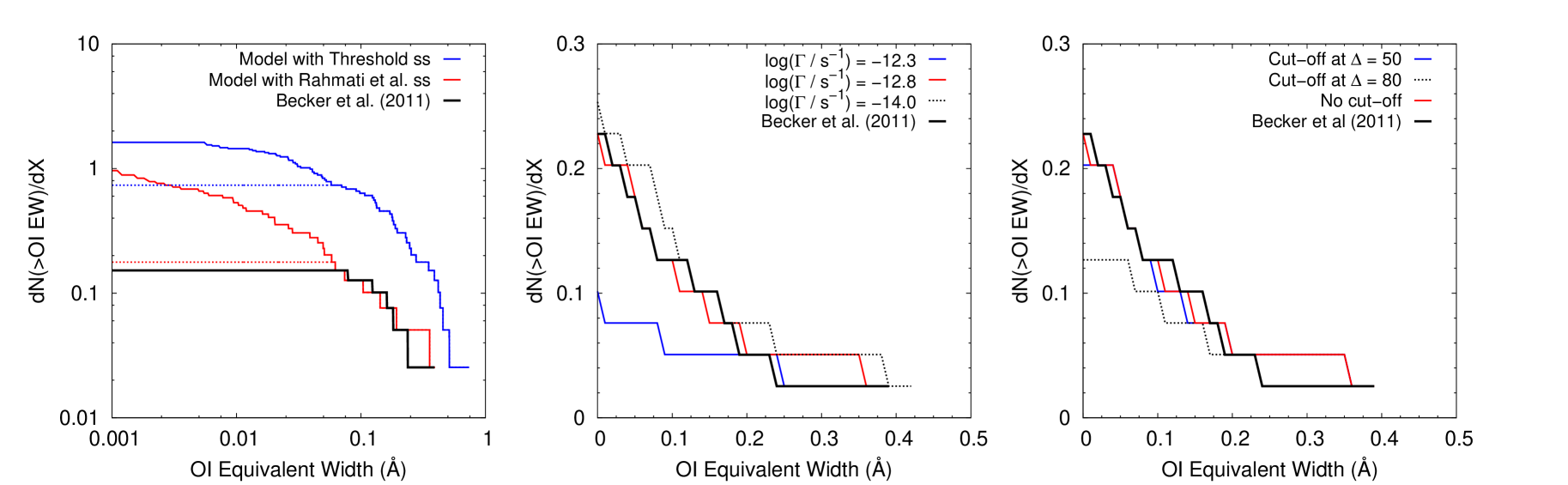
Figure 5: The cumulative incidence rate of simulated O i absorbers compared to the observed distribution obtained by Becker et al. (2011). The left panel is for the metallicity model that fits the data with the Rahmati et al. (2013a) self shielding model ($Z=10^{-2.65}\,Z_{\odot}\,(\Delta/80)^{1.3}$). The dashed/solid curves are with/without the Becker et al. completeness correction. The middle panel shows the cumulative incidence rate of simulated O i absorbers assuming different background photo-ionization rates $\Gamma$ and the Rahmati et al. (2013a) self-shielding model. The completeness correction shown in the right panel of Fig. 4 has been applied to the curves. The metallicity model used is the same as in the left panel. The right panel shows the effect of introducing different cut-off overdensities, below which the metallicity is set to zero. The red curve assumes a power law model for the metallicity that extends to arbitrarily low density. The blue curve assumes that regions with $\Delta<50$ contain no metals. The black dashed curve assumes that there are no metals below a cut-off overdensity of $\Delta=80$. The thick black curve shows the observed cumulative incidence rate of O i absorbers obtained by Becker et al. (2011). The metallicity model used is the same as in the left panel.

For a quantitative comparison with the simulated O i absorption to the Becker et al. (2011) sample, we have compiled cumulative incidence rates as shown in Figure 5. The parameters of the assumed metallicity density relation were chosen to give a good match to the data for our fiducial photo-ionization rate $\log(\Gamma/\textnormal{s}^{-1})=-12.8$, a value consistent with the observations at $z=6$ as shown in the right panel of Figure 1 (Calverley et al., 2011; Wyithe & Bolton, 2011). The left panel of Figure 5 shows the cumulative distribution with and without applying the completeness correction to the sample of simulated O i spectra. As the left panel shows, a metallicity-density relation with $Z_{80}=10^{-2.65}\,Z_{\odot}$ gives a good match to the data for the Rahmati et al. (2013a) self-shielding model.

We have also tested the effect of using the threshold density for self-shielding instead of the Rahmati et al. (2013a) prescription. With the threshold self-shielding model, self-shielded regions have a larger covering factor. There are therefore many more O i absorbers of a given EW and the EW distribution extends to larger values for the same metallicity. It is possible to fit the observed EW distribution of the observed O i absorbers with either of the two self-shielding prescriptions we have implemented, but, as we discuss in more detail in section 4.1, the inferred metallicity differs significantly. As the Rahmati et al. (2013a) prescription includes radiative transfer effects, we will consider our simulations with this prescription to be our fiducial self-shielding model.

In the middle panel of Figure 5, we show how changing $\Gamma$ affects the cumulative incidence rate. The number of lines seen at small equivalent widths increases strongly as $\Gamma$ decreases, but the number of lines seen at larger equivalent widths is insensitive to changes in $\Gamma$. We have tested a wide range of $\Gamma$. The incidence rate of weak O i absorbers decreases rapidly with increasing photo-ionization rate, compared to our fiducial value of $\log(\Gamma/\textnormal{s}^{-1})=-12.8$. When we decrease the photo-ionization rate, the incidence rate quickly saturates once the O i absorbers have become fully neutral. We show here two extreme cases with $\log(\Gamma/\textnormal{s}^{-1})=(-12.3,-14.0)$, which represent a highly ionized and significantly neutral IGM, respectively.

The right panel of Figure 5 shows the effect of applying a cut-off to the metallicity at different overdensities. Below this cut-off, it is assumed that no metals are present. Above this cut-off, the metallicity follows the power-law model as before. The simulations of Finlator et al. (2013) which attempt to model the metal transport into low density regions predict such a cut-off. The details of this cut-off will, however, depend sensitively on the details of the galactic wind implementations in numerical simulations. A cut-off of $\Delta=80$ (0.003% of simulation volume) produced too few simulated O i absorbers compared to the Becker et al. (2011) survey. A cut-off of $\Delta=50$ (0.01% of simulation volume) made only a small difference compared to not using a cut-off at all. This suggests that the metals have travelled out to regions with overdensities as low as $\Delta\sim 50-80$ by $z\sim 6$ and that the metallicity at lower densities is not (yet) probed by the current data. Note that the effect of a high cut-off overdensity is similar to that of a high $\Gamma$.

We have also compared the velocity widths, $\Delta v_{90}$, of the simulated O i absorption to that of the Becker et al. (2011) survey. For this we have identified the velocity interval covering 90% of the optical depth in the O i absorption systems. The velocity widths of our simulated O i absorbers range from $18.5\,\rm km\,\rm s^{-1}$ for a line with equivalent width $W_{\lambda}=0.02\,\textnormal{\AA}$ to $45.0\,\rm km\,\rm s^{-1}$ for a line with equivalent width $W_{\lambda}=0.06\,\textnormal{\AA}$. These $\Delta v_{90}$ values are similar to the velocity widths measured by Becker et al. (2011) for their observed O i absorption lines.

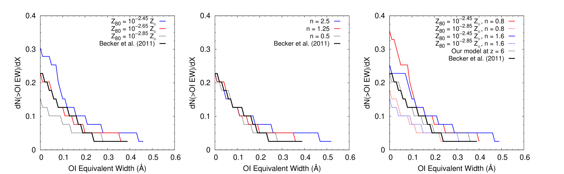
Figure 6: The cumulative incidence rate of O i absorbers showing the effect of changing slope and normalization of the metallicity model ($Z=Z_{80}\,(\Delta/80)^{n}$). All curves shown have a completeness correction applied. The assumed photo-ionization rate for the simulated O i absorbers is $\log(\Gamma/\textnormal{s}^{-1})=-12.8$ and the Rahmati et al. (2013a) self-shielding model was used. The left panel shows the effect of varying the normalisation $Z_{80}$. The middle panel shows the effect of changing the power law index $n$. The right panel shows the four metallicity models that define the blue-shaded region in the left panel of Figure 7.

Varying $Z_{80}$ and $n$ in the model of the metallicity, as well as changing $\Gamma$, both have very noticeable effects on the number of absorption lines produced by the simulation. As shown in Figure 6, increasing the normalisation $Z_{80}$ (left panel) does not change the slope of the cumulative distribution while varying the power law index $n$ does. The maximum equivalent width seen in the simulation decreases with decreasing $n$. While some degeneracy exists between $Z_{80}$ and $n$, therefore, we have some leverage with which to constrain these parameters by matching both the slope and the amplitude of the observed distribution.

4 Results

4.1 The metallicity and photo-ionization rate at $z\sim 6$

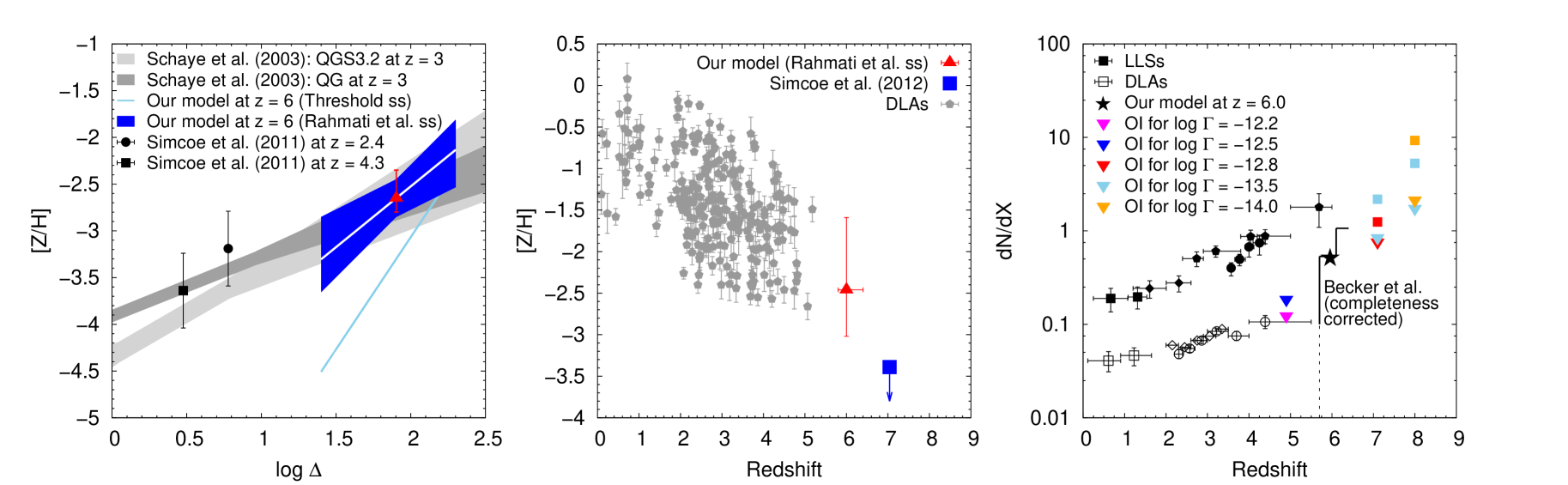
Figure 7: Left: The dark blue shaded region and the light blue line show the metallicity inferred as a function of overdensity for the Rahmati et al. (2013a) and the threshold self-shielding model, respectively. The dark blue shaded region is thereby defined by the four metallicity models shown in the right panel of Figure 6 and the central white line is our fiducial metallicity model. The assumed photo-ionization rate is $\log(\Gamma/\textnormal{s}^{-1})=-12.8$ and the value of the inferred $Z_{80}$ for our fiducial metallicity model is denoted by the red triangle. The red bar shows how the inferred $Z_{80}$ increases using the Rahmati et al. (2013a) self-shielding model as the photionization rate is increased in the range $\log(\Gamma/\textnormal{s}^{-1})=(-13.5,-12.5)$. Also shown is the metallicity as a function of overdensity at $z=3$, as measured by Schaye et al. (2003), in grey for two different models of the UV background and measurements of the metallicity of the IGM by Simcoe (2011). Middle: The red triangle shows the median $z\sim 6$ metallicity of completeness-corrected simulated O i absorbers with EW${}_{\textnormal{\scriptsize{OI}}}\geq 0.01$ for our fiducial model as measured by comparing total O i and H i column density. The vertical error bar represents the $1\sigma$ range of metallicities of the simulated absorbers, while the horizontal error bar indicates the redshift range of the O i absorbers observed by Becker et al. (2011). The grey points show a compilation of metallicity measurements of DLAs compiled in Rafelski et al. (2012). The upper limit for the metallicity measured by Simcoe et al. (2012) for a possible proximate DLA in the foreground of the $z=7.085$ QSO ULASJ1120+0641 is also shown. Right: Comparison of the predicted evolution of the incidence rate ${\rm d}N/{\rm d}X$ of our simulated O i absorbers with EW${}_{\textnormal{\scriptsize{OI}}}\geq 0.01\,\mathrm{\AA}$ and and that of observed LLSs (black points) and DLAs (open points). The square points at $z=7$ and $z=8$ show predictions for the incidence rate of OI absorbers with a threshold EW${}_{\textnormal{\scriptsize{OI}}}=0.001\,\mathrm{\AA}$. LLSs: Songaila & Cowie (2010) and as compiled in Fumagalli et al. (2013). DLAs: As compiled in Seyffert et al. (2013).

In the left panel of Figure 7 we show the metallicity-density relation of our fiducial model which reproduces the incidence rate of the observed O i absorbers and compare it to that measured by Schaye et al. (2003) at $z=3$ for two plausible models of the UV background at this redshift, as well as to those of Simcoe (2011) at $z=2.4$ and $z=4.3$. Note that these metallcities have been lowered by 0.12 and 0.09 dex, respectively, to match the Asplund et al. (2009) measurements of solar abundances assumed here.

Our fiducial metallicity density relation, utilizing the Rahmati et al. (2013a) self-shielding model, is given by,

$$Z=10^{-2.65}\,Z_{\odot}\left(\frac{\Delta}{80}\right)^{1.3},$$ (5)

with a background photo-ionization rate $\log(\Gamma/\textnormal{s}^{-1})=-12.8$. This relation was determined by calculating ${\rm d}N(>{\rm EW}_{\rm OI})/{\rm d}X$ and the maximum O i EW for a range of $Z_{80}$ and $n$ and finding the best match to the observations of Becker et al. (2011) with a K-S test.

Rather surprisingly, our modelling of the O i absorbers suggests that there is little, if any, evolution of the metallicities of the CGM between $3<z<6$ in the overdensity range probed by the O i absorbers. Note, however, that our assumption of no scatter in the metallicity density relation is certainly not realistic. We will come back to this later. For reference, we also show the inferred metallicities for the threshold self-shielding model. As already discussed, the metallicities are typically a factor of ten lower (with a steeper density dependence) due to the larger neutral fractions in this model.

When varying the metallicity distribution and photo-ionization rate, we found a rather weak dependence of the O i incidence rate on the latter, which was degenerate with adjusting the metal distribution unless the photo-ionization was so high that the gas in self-shielded region became highly ionized and their incidence rate too low to reproduce the Becker et al. (2011) data. That occurred at $\log\Gamma\ga-12.4$. The red bar in the left panel of Figure 7 shows how the inferred $Z_{80}$ changes as the photo ionization rate varies in the range $-13.5<\log(\Gamma/\textnormal{s}^{-1})<-12.5$. As expected, the inferred metallicity thereby increases with increasing photo-ionization rate (the value denoted by the red triangle is for our fiducial model with $\log(\Gamma/\textnormal{s}^{-1})=-12.8$ suggested by measurements of the photo-ionization rate from Lyman-$\alpha$ forest data). The dependence of the inferred metallicity on the assumed photo-ionization rate is thereby weak (a change of 0.5 dex in inferred metallicity for a change of 1.6 dex of the photo-ionization rate). We also note again that modelling the self-shielding carefully is important. With the simple threshold self-shielding model the normalization of the inferred metallicity at the characteristic overdensity $\Delta=80$ would be 0.8 dex lower and the inferred dependence on overdensity would be significantly steeper than for the Rahmati et al. (2013a) self-shielding model.

The number of observed O i absorbers is still far too small for a robust determination of the differential O i EW distribution and its errors, but as we will discuss in more detail in section 4.5, the main uncertainties in the inferred metallicity are anyway due to still uncertain model assumptions as e.g. demonstrated in Figure 7 by the sensitivity to the details of the self-shielding model and the assumed photo-ionization rate. We have thus not attempted to calculate formal confidence intervals for $Z_{80}$ and $n$. The blue shaded region in the left panel of Figure 7 shows instead a range of metallicity density relations at fixed photo-ionization rate for which we show the corresponding cumulative O i incidence rate in the right panel of Figure 6.

In the middle panel of Figure 7, we compare the metallicity that would be measured along lines of sight through our simulation that contain O i absorbers by comparing the total O i and H i column densities with the measured metallicity of DLAs at a range of redshifts. Our inferred metallicity for the O i absorbers is at the lower end of the range of measured DLAs at somewhat lower redshift. This should not be surprising given the sub-DLA column densities we have inferred for the O i absorbers which should probe the CGM at somewhat lower overdensities and larger distances from the host galaxy than the DLAs. We also show the upper limit for the metallicity obtained by Simcoe et al. (2012) for the case that the damping wing redwards of Lyman-$\alpha$ in the $z=7.085$ QSO ULASJ1120+0641 is interpreted as due to a proximate foreground DLA at $z=7.041$. This upper limit is significantly below our estimate for the metallicity of the O i absorbers. We have also calculated predicted metallicities for absorbers with $\log N_{\textnormal{\scriptsize{HI}}}\geq 20.45$ (the column density range inferred by Simcoe et al. (2012)) for our fiducial metallicity model and photo-ionization rates $-14.0\leq\log\Gamma\leq 12.8$ and found them to be a factor three or more higher than the upper limit on the metallicity inferred by Simcoe et al. (2012). This renders the interpretation as a proximate foreground DLA rather unlikely (see also BH13 and the corresponding discussion in Finlator et al. (2013) who come to similar conclusions), but we should note again here that we made no attempt to model the likely scatter in metallicity of the CGM in our simulations.

4.2 The relation to lower redshift DLAs and LLSs

In the right panel of Figure 7, we compare the redshift evolution of the incidence rate of our modelled O i absorbers for a range of plausible assumptions of the photo-ionization rate to the evolution of the incidence of LLSs and DLAs at lower redshift. As already discussed by Becker et al. (2011), the incidence rate of their observed O i absorbers at $z=6$ is similar to that of LLSs at $z=4$. The incidence rate of our simulated O i absorbers at $z=5$ matches very well with that of observed DLAs and LLSs at lower redshift. At $z>5$ the photo-ionization rate appears to drop (right panel of Figure 1; Wyithe & Bolton 2011; Calverley et al. 2011) which can be mainly attributed to a rapidly decreasing mean free path with increasing redshift as the tail-end of reionization is approached (McQuinn, Oh & Faucher-Giguère, 2011). If we assume such a drop of the photo-ionization rate our simulations reproduce the rapid evolution of the incidence rate of the O i absorbers in the Becker et al. (2011) data very well. As we will discuss in more detail in the next section, the rapid evolution of the incidence rate of the simulated O i absorbers is expected to continue at $z>6$. Inspection of Figure 2 further shows that the incidence rate depends more strongly on the photo-ionization rate and only to a lesser extent on the increasing density with redshift. This explains e.g. the rather small difference in the incidence rates of our modelled O i absorbers at $z=6$ and $z=7$ for our fiducial photo-ionization rate ($\log\Gamma=-12.8$) shown by the star and the red triangle in the right panel of 7, respectively.

4.3 The spatial distribution of O i absorbers

Figure 8 shows the spatial distribution of the O i EW for our models for a range of redshifts and photo-ionization rates. For this we have calculated H i column densities by integrating the neutral hydrogen density as shown in Figure 2 with the Rahmati et al. (2013a) self-shielding model over the thickness of the slice shown and used the correlation between H i column density and O i EW in the middle panel of Figure 4 to translate the H i column densities into O i equivalent widths. The relation used was

$$\log\mathrm{EW_{OI}}=2.51\log N_{\scriptsize{\mathrm{HI}}}-47.86.$$ (6)

The black contours shows the location of O i absorbers with ${\rm EW}_{\scriptsize{\mathrm{OI}}}\geq 0.01\,\mathrm{\AA}$. Figure 8 suggests that the observed absorbers at $z\sim 6$ indeed probe the (outer parts) of the haloes of (faint) high-redshift galaxies as suggested by Becker et al. (2011). If the metal distribution extends to lower densities than currently probed the O i absorbers are expected to start to probe more and more the filamentary structures connecting these galaxies as the meta-galactic photo-ionization rate decreases and the Universe becomes increasingly more neutral with increasing redshift.

4.4 Predictions for the incidence rate of O i absorbers at $z=7$ and beyond

We have also used our simulations to predict the evolution of the number of absorption systems at $z=7$ and $z=8$. For this we assumed the inferred metallicity-(over)density relation at $z=6$. This seems to be a reasonable assumption given the apparent absence of a metallicity evolution at the relevant densities between $z=3$ and $z=6$.

Figure 8: The location of O i absorbers in the simulation. The O i equivalent width was estimated from the H i column density (see Figure 4). The H i column density was calculated by integrating $n_{\rm HI}$ over the thickness ($39h^{-1}\,\mathrm{ckpc}$) of the slice shown in the plot. The distribution of O i absorbers is shown for $\log\Gamma=-12.8$ at $z=(6.0,7.1)$, for $\log\Gamma=-13.5$ for $z=7.1$ and for $\log\Gamma=-14.0$ at $z=8.0$. The Rahmati et al. (2013a) model for self-shielding was used in each case. The black contours enclose absorbers with ${\rm EW}_{\scriptsize{\mathrm{OI}}}\geq 0.01\,\mathrm{\AA}$.

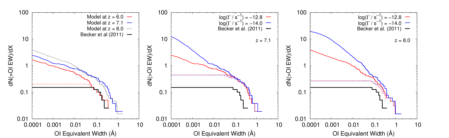
Figure 9: Left: The solid red and blue lines and the black dashed line show the predicted cumulative incidence rate of O i absorbers without completeness correction for the metallicity distribution that fits the observed distribution well at $z=6.0$ with the Rahmati et al. (2013a) self-shielding model and $\log(\Gamma/\textnormal{s}^{-1})=-12.8$. The red dashed curve is for the simulated O i absorbers at $z=6.0$ with the completeness correction applied. The thick black curve is the Becker et al. (2011) data. Middle: The thin solid lines show the predicted cumulative incidence rate of O i absorbers without completeness correction for different values of the background photo-ionization rate at $z=7.1$. The dashed curves show the effect of applying a cut-off in the metallicity below $\Delta=50$. Right: The thin solid lines show the predicted cumulative incidence rate of O i absorbers without completeness correction for different values of the background photo-ionization rate at $z=8.0$. The dashed curves show the effect of applying a cut-off in the metallicity model below $\Delta=50$.

The left panel of Figure 9 shows a cumulative plot for the incidence rate ${\rm d}N(>{\rm EW}_{\rm OI})/{\rm d}X$ for our modelling at $z=(6.0,7.1,8.0)$ for a fixed photo-ionization rate, $\log(\Gamma/\textnormal{s}^{-1})=-12.8$. The results for $z=6$ are shown in red with (dotted curve) and without (solid curve) completeness correction, while the results at $z=7.1$ and $z=8.0$ are shown only without the Becker et al. (2011) completeness correction as the blue solid and black dotted curve, respectively. The significant, but moderate evolution is here only due to the increasing (column) densities with increasing redshift.

The two right panels of Figure 9 show the cumulative incidence rate for two background photo-ionization rates at $z=7.1$ and $z=8.0$, respectively. The solid lines represent metallicity models with no cut-off and the dashed lines represent models with a cut-off for the presence of metals at $\Delta=50$. If the presence of metals should indeed be limited to overdensities $\Delta\geq 50$, the total incidence rate saturates at ${\rm d}N(>{\rm EW}_{\rm OI})/{\rm d}X\sim 0.5$ and there is very little, if any, sensitivity to a decrease in the photo-ionization rate. The EW of the weakest O i absorbers is $0.01\,\mathrm{\AA}$, not much larger than the weakest absorbers detected by Becker et al. (2011) at $z\sim 6$. This is because, in this case, increasing redshift and/or decreasing photo-ionization rate increase only moderately the covering factor of self-shielded regions that contain metals. If, instead, the presence of metals follows our assumed power-law metallicity-density relation all the way to low densities, there will be a larger number of additional weak O i absorbers and the total incidence rate increases by about a factor of ten to ${\rm d}N(>{\rm EW}_{\rm OI})/{\rm d}X\sim 10$ for O i absorbers with EW $>0.001\,\mathrm{\AA}$. In this case the weakest absorbers remain sensitive to the value of the decreasing photo-ionization rate. Note, however, that pushing to such small O i EW will almost certainly require a 30m telescope. Note further that by assuming that the metallicity does not evolve with redshift our predictions are optimistic and smaller numbers of O i absorbers would be expected if the metallicity of the CGM/IGM were to decrease over the redshift range considered.

4.5 Caveats

In this work, we have made a number of simplifying assumptions which may have affected our results. Most critical is probably our approximate treatment of radiative transfer effects, especially for our predictions towards higher redshift where we move deeper into the epoch of reionization.

• Our treatment of self-shielding is based on the full radiative transfer simulations of Rahmati et al. (2013a) and should be reasonably accurate as long as internal sources within the O i absorbers do not dominate the ionizing flux. Rahmati et al. (2013b) have investigated the effect of local stellar ionizing radiation and found that it can have a significant effect for LLSs and sub-DLAs (see also Kohler & Gnedin 2007). This may mean that we have somewhat underestimated the metallicity necessary to produce the observed O i absorbers.

• Our assumption of a fixed metallicity-density relation is also certainly not correct. From observations of DLAs, we know that the metallicity scatter in absorbers with larger column density is significant. We should expect this to be the case also for the O i absorbers, which are essentially sub-DLAs. In a self-consistent picture for the ionizing sources and the production and transport of metals one may even expect an anti-correlation between metallicity and the amout of neutral gas present.

• Our simulations also neglect the effect of outflows on the gas distribution. There may thus be overall less gas at the impact parameters producing O i absorbers than our simulations predict and this may lead to a systematic underestimate of metallicites. Note that the simulations by Rahmati et al. (2013a) did include the effect of galactic winds.

• Somewhat problematic is also the rather small box size of our simulations, which is dictated by the need to resolve the small scale filamentary structures which dominate the absorption signatures in QSO spectra at high redshift (see Bolton & Becker (2009) for a detailed discussion). There should thus also be more scatter in the correlation between overdensity and hydrogen column density than our simulations suggest.

• For our predictions towards higher redshift, the neglect of the expected substantial fluctuations of the photo-ionization rate is another issue. The expected number of O i absorbers should vary greatly on scales of the mean free path of ionizing photons, which becomes comparable or smaller than the box size of our simulations at $z\ga 6$.

4.6 Comparison to other work

Detailed simulations of O i absorption at the tail-end of reionization are still in their infancy. Most notably, Finlator et al. (2013) have recently presented full cosmological radiative transfer simulations which also follow the metal enrichment history of the circumgalactic medium. The relevant processes (reionization, metal transport by galactic winds) are difficult to simulate from first principles and it is perhaps not surprising that Finlator et al. (2013) were somewhat struggling to reproduce the observed O i absorbers by Becker et al. (2011). As far as we can tell from comparing their work to ours, the main difference is – as the authors point out themselves – that in their simulations the build-up of the meta-galactic UV background had progressed already too far by $z\sim 6$. This then leaves too little neutral gas in self-shielded regions. In contrast to our findings, Finlator et al. (2013) also predict a decrease of the incidence rate of O i absorbers with increasing redshift. The difference here can be traced to the fact that, in their simulations, the filamentary structure connecting the DM haloes hosting their galaxies is not metal enriched and/or substantially neutral. Finally, we should note that the metallicity in their simulation at $z\sim 6$ is about a factor of ten higher than we infer at the relevant overdensities at the same redshift perhaps suggesting that the implementation of galactic winds in their simulations does not transport metals to sufficiently large distances.

5 Summary and conclusions

We have used cosmological hydrodynamical simulations to model the neutral hydrogen and the associated OI absorption in regions of the circumgalactic medium at high redshift. A simple power-law metallicity-density relation was assumed. The self-shielding to ionizing radiation was modelled by post-processing the simulations using two different schemes. Our simulations reproduce the incidence rate of observed O i absorbers at $z=6$ and their cumulative incidence rate with a metallicity [O/H] $\sim-2.7$ at a typical overdensity $\Delta=80$, with the presence of oxygen extending to an overdensity at least as low as $\Delta\sim 50-80$, a moderate density dependence with power-law index $n=1.3$, and a photo-ionization rate in agreement with measurements from Lyman-$\alpha$ forest data, $\log(\Gamma/\textnormal{s}^{-1})=-12.8$. The metallicity we infer here is very similar to that inferred by Schaye et al. (2003) at $z\sim 3$ from C iv absorption by (highly ionized) gas at a similar overdensity. There appears, therefore, to be remarkably little evolution of the typical metallicity of the CGM between $3<z<6$ at these overdensities. The efficient metal enrichment of the CGM appears to have started early in the history of the Universe and in low-mass galaxies. Our inferred metallicity is also in good agreement with the lower end of those of DLAs at slightly lower redshift. This gives further support to a picture where the observed O i absorption arises at somewhat larger impact parameter and lower overdensity with somewhat lower column density than typical DLAs.

Our simulations further reproduce the observed rapid redshift evolution of observed O i absorbers at $z>5$ for reasonable assumptions for the evolution of the meta-galactic photo-ionization rate. The rapid evolution is mainly due to the self-shielding threshold moving out first from the inner part into the outer part of galactic haloes and then into the filamentary structures of the cosmic web. This is due to the decreasing photo-ionization rate as we progress deeper into the epoch of reionization with increasing redshift. The observed evolution of the incidence rate of O i absorbers thereby matches well onto that of LLSs and DLAs at lower redshift.

Finally, we have made predictions for the expected number of O i absorbers at redshifts larger than currently observed and predict that the rapid evolution will continue with increasing redshift as the O i absorbers probe the increasingly neutral cosmic web. Pushing the detection of O i absorbers to higher redshift ($z>6$) and lower EW should therefore provide a rich harvest and should allow unique insight into the enrichment history of the circumgalactic medium and the details of how reionization proceeds.

Appendix A O I as a tracer of H I

We have used the photo-ionization code CLOUDY (Ferland et al., 1998) to estimate the neutral oxygen fraction as a function of H i column density. The blue solid curve shows the the ratio of the neutral fractions of oxygen and hydrogen $f_{\mathrm{OI}/\mathrm{HI}}=f_{\mathrm{OI}}/f_{\mathrm{HI}}$ for a slab of constant density illuminated from the outside with the Haardt & Madau (2012) model for the UV background, which includes contributions from quasars and galaxies. The simulations were performed at $z=6$ and the effects of the CMB and background cosmic rays were also taken into account. We further assumed an equation of state with constant pressure. The result is very similar to that obtained for the Haardt & Madau (2001) UV background model shown by the black curve. In order to test the sensitivity to the amplitude of of the UV background and the temperature of the gas we also show the results with the UV intensity increased/decreased by a factor of three and for fixed temperatures of 5000K and 10000K with the dot-dashed and dotted curves as indicated on the plot. The results were found to be insensitive to the number density of hydrogen in the slab.

For column densities $\log N_{\mathrm{HI}}\ga 17$, where the gas is self-shielded, the neutral fraction of oxygen traces that of hydrogen very well (to within 0.1 dex or better) independent of the detailed assumptions of our CLOUDY calculations. This is unsurprising since at $z\sim 6$, the main contributuion to the ionizing background is from galaxies and is therefore relatively soft. For harder ionizing spectra, $f_{\mathrm{OI}/\mathrm{HI}}$ would begin to decline at higher column densities. At smaller H i column densities, the neutral fraction of oxygen drops significantly faster than that of hydrogen and $f_{\mathrm{OI}/\mathrm{HI}}$ depends on the amplitude of the UV background, but is very similar for the two background UV models we tested. It also changes little for our two constant temperature calculations. We should note here that non-selfshielded regions contribute, however, negligibly to the O i absorbers discussed in the main paper.

We have adopted the calculation with the Haardt & Madau (2012) model of the UV background as our fiducial model for the calculation of the O i absorption in our simulations. We produced a set of interpolation tables that were used in the relationship $n_{\mathrm{OI}}=Z_{\mathrm{O}}\,f_{\mathrm{OI/HI}}\,n_{\mathrm{HI}}$ (Section 3.1) for each O i absorber.

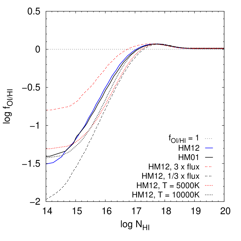
Figure 10: Plot of the neutral fraction of oxygen relative to the neutral fraction of hydrogen against H i column density. The blue curve assumes the Haardt & Madau (2012) UV backround model. We find that O i is a good tracer of H i for self-shielded gas with $\log N_{\mathrm{HI}}\ga 17$. Calculations for the Haardt & Madau (2001) model of the UV background and for decreased/increased amplitude of the UV background and constant temperature of the gas of 5000K and 10000K are also shown. The dashed line shows $f_{\mathrm{OI}/\mathrm{HI}}=1$.

References

- Abel et al. (1997) Abel T., Anninos P., Zhang Y., Norman M. L., 1997, New A, 2, 181
- Akerman et al. (2005) Akerman C. J., Ellison S. L., Pettini M., Steidel C. C., 2005, A&A, 440, 499
- Asplund et al. (2009) Asplund M., Grevesse N., Sauval A. J., Scott P., 2009, ARA&A, 47, 481
- Bahcall & Peebles (1969) Bahcall J. N., Peebles P. J. E., 1969, ApJ, 156, L7
- Becker & Bolton (2013) Becker G. D., Bolton J. S., 2013, MNRAS, 436, 1023
- Becker, Rauch & Sargent (2007) Becker G. D., Rauch M., Sargent W. L. W., 2007, ApJ, 662, 72
- Becker et al. (2011) Becker G. D., Sargent W. L. W., Rauch M., Calverley A. P., 2011, ApJ, 735, 93
- Boisse et al. (1998) Boisse P., Le Brun V., Bergeron J., Deharveng J.-M., 1998, A&A, 333, 841
- Bolton & Becker (2009) Bolton J. S., Becker G. D., 2009, MNRAS, 398, L26
- Bolton & Haehnelt (2007) Bolton J. S., Haehnelt M. G., 2007, MNRAS, 374, 493
- Bolton & Haehnelt (2013) Bolton J. S., Haehnelt M. G., 2013, MNRAS, 429, 1695
- Calverley et al. (2011) Calverley A. P., Becker G. D., Haehnelt M. G., Bolton J. S., 2011, MNRAS, 412, 2543
- Centurión et al. (2003) Centurión M., Molaro P., Vladilo G., Péroux C., Levshakov S. A., D’Odorico V., 2003, A&A, 403, 55
- Churchill et al. (2000) Churchill C. W., Mellon R. R., Charlton J. C., Jannuzi B. T., Kirhakos S., Steidel C. C., Schneider D. P., 2000, ApJS, 130, 91
- Dessauges-Zavadsky et al. (2004) Dessauges-Zavadsky M., Calura F., Prochaska J. X., D’Odorico S., Matteucci F., 2004, A&A, 416, 79
- Dessauges-Zavadsky et al. (2007) Dessauges-Zavadsky M., Calura F., Prochaska J. X., D’Odorico S., Matteucci F., 2007, A&A, 470, 431
- Dessauges-Zavadsky et al. (2001) Dessauges-Zavadsky M., D’Odorico S., McMahon R. G., Molaro P., Ledoux C., Péroux C., Storrie-Lombardi L. J., 2001, A&A, 370, 426
- Dessauges-Zavadsky et al. (2006) Dessauges-Zavadsky M., Prochaska J. X., D’Odorico S., Calura F., Matteucci F., 2006, A&A, 445, 93
- Ellison et al. (2007) Ellison S. L., Hennawi J. F., Martin C. L., Sommer-Larsen J., 2007, MNRAS, 378, 801
- Ellison et al. (2001) Ellison S. L., Pettini M., Steidel C. C., Shapley A. E., 2001, ApJ, 549, 770
- Fan et al. (2006) Fan X. et al., 2006, AJ, 132, 117
- Ferland et al. (1998) Ferland G. J., Korista K. T., Verner D. A., Ferguson J. W., Kingdon J. B., Verner E. M., 1998, PASP, 110, 761
- Finlator et al. (2013) Finlator K., Muñoz J. A., Oppenheimer B. D., Oh S. P., Özel F., Davé R., 2013, MNRAS, 436, 1818
- Fumagalli et al. (2013) Fumagalli M., O’Meara J. M., Prochaska J. X., Worseck G., 2013, ApJ, 775, 78
- Green (2011) Green D. A., 2011, Bulletin of the Astronomical Society of India, 39, 289
- Haardt & Madau (2001) Haardt F., Madau P., 2001, in Clusters of Galaxies and the High Redshift Universe, Neumann D. M., Tran J. T. V., eds.
- Haardt & Madau (2012) Haardt F., Madau P., 2012, ApJ, 746, 125
- Haehnelt, Steinmetz & Rauch (1998) Haehnelt M. G., Steinmetz M., Rauch M., 1998, ApJ, 495, 647
- Jorgenson, Wolfe & Prochaska (2010) Jorgenson R. A., Wolfe A. M., Prochaska J. X., 2010, ApJ, 722, 460
- Khare et al. (2004) Khare P., Kulkarni V. P., Lauroesch J. T., York D. G., Crotts A. P. S., Nakamura O., 2004, ApJ, 616, 86
- Kohler & Gnedin (2007) Kohler K., Gnedin N. Y., 2007, ApJ, 655, 685
- Kulkarni et al. (2013) Kulkarni G., Rollinde E., Hennawi J. F., Vangioni E., 2013, ApJ, 772, 93
- Kulkarni et al. (2005) Kulkarni V. P., Fall S. M., Lauroesch J. T., York D. G., Welty D. E., Khare P., Truran J. W., 2005, ApJ, 618, 68
- Ledoux, Bergeron & Petitjean (2002) Ledoux C., Bergeron J., Petitjean P., 2002, A&A, 385, 802
- Ledoux et al. (2006) Ledoux C., Petitjean P., Fynbo J. P. U., Møller P., Srianand R., 2006, A&A, 457, 71
- Ledoux, Petitjean & Srianand (2003) Ledoux C., Petitjean P., Srianand R., 2003, MNRAS, 346, 209
- Ledoux, Srianand & Petitjean (2002) Ledoux C., Srianand R., Petitjean P., 2002, A&A, 392, 781
- Levshakov et al. (2002) Levshakov S. A., Dessauges-Zavadsky M., D’Odorico S., Molaro P., 2002, ApJ, 565, 696
- Lopez & Ellison (2003) Lopez S., Ellison S. L., 2003, A&A, 403, 573
- Lopez et al. (2002) Lopez S., Reimers D., D’Odorico S., Prochaska J. X., 2002, A&A, 385, 778
- Lopez et al. (1999) Lopez S., Reimers D., Rauch M., Sargent W. L. W., Smette A., 1999, ApJ, 513, 598
- Lu, Sargent & Barlow (1998) Lu L., Sargent W. L. W., Barlow T. A., 1998, AJ, 115, 55
- Lu et al. (1996) Lu L., Sargent W. L. W., Barlow T. A., Churchill C. W., Vogt S. S., 1996, ApJS, 107, 475
- Maio, Ciardi & Müller (2013) Maio U., Ciardi B., Müller V., 2013, MNRAS, 435, 1443
- McQuinn et al. (2008) McQuinn M., Lidz A., Zaldarriaga M., Hernquist L., Dutta S., 2008, MNRAS, 388, 1101
- McQuinn, Oh & Faucher-Giguère (2011) McQuinn M., Oh S. P., Faucher-Giguère C.-A., 2011, ApJ, 743, 82
- Meiring et al. (2006) Meiring J. D. et al., 2006, MNRAS, 370, 43
- Meiring et al. (2007) Meiring J. D., Lauroesch J. T., Kulkarni V. P., Péroux C., Khare P., York D. G., Crotts A. P. S., 2007, MNRAS, 376, 557
- Meiring et al. (2011) Meiring J. D. et al., 2011, ApJ, 732, 35
- Mesinger (2010) Mesinger A., 2010, MNRAS, 407, 1328
- Meyer, Lanzetta & Wolfe (1995) Meyer D. M., Lanzetta K. M., Wolfe A. M., 1995, ApJ, 451, L13
- Miralda-Escudé, Haehnelt & Rees (2000) Miralda-Escudé J., Haehnelt M., Rees M. J., 2000, ApJ, 530, 1
- Molaro et al. (2000) Molaro P., Bonifacio P., Centurión M., D’Odorico S., Vladilo G., Santin P., Di Marcantonio P., 2000, ApJ, 541, 54
- Molaro et al. (2001) Molaro P., Levshakov S. A., D’Odorico S., Bonifacio P., Centurión M., 2001, ApJ, 549, 90
- Mortlock et al. (2011) Mortlock D. J. et al., 2011, Nature, 474, 616
- Nestor et al. (2008) Nestor D. B., Pettini M., Hewett P. C., Rao S., Wild V., 2008, MNRAS, 390, 1670
- Noterdaeme et al. (2008) Noterdaeme P., Ledoux C., Petitjean P., Srianand R., 2008, A&A, 481, 327
- Noterdaeme et al. (2012) Noterdaeme P. et al., 2012, A&A, 547, L1
- Oh (2002) Oh S. P., 2002, MNRAS, 336, 1021
- O’Meara et al. (2013) O’Meara J. M., Prochaska J. X., Worseck G., Chen H.-W., Madau P., 2013, ApJ, 765, 137
- Péroux et al. (2006) Péroux C., Meiring J. D., Kulkarni V. P., Ferlet R., Khare P., Lauroesch J. T., Vladilo G., York D. G., 2006, MNRAS, 372, 369
- Péroux et al. (2008) Péroux C., Meiring J. D., Kulkarni V. P., Khare P., Lauroesch J. T., Vladilo G., York D. G., 2008, MNRAS, 386, 2209
- Petitjean, Srianand & Ledoux (2000) Petitjean P., Srianand R., Ledoux C., 2000, A&A, 364, L26
- Petitjean, Srianand & Ledoux (2002) Petitjean P., Srianand R., Ledoux C., 2002, MNRAS, 332, 383
- Pettini et al. (1999) Pettini M., Ellison S. L., Steidel C. C., Bowen D. V., 1999, ApJ, 510, 576
- Pettini et al. (2000) Pettini M., Ellison S. L., Steidel C. C., Shapley A. E., Bowen D. V., 2000, ApJ, 532, 65
- Prochaska & Burles (1999) Prochaska J. X., Burles S. M., 1999, AJ, 117, 1957
- Prochaska, Gawiser & Wolfe (2001) Prochaska J. X., Gawiser E., Wolfe A. M., 2001, ApJ, 552, 99
- Prochaska et al. (2003a) Prochaska J. X., Gawiser E., Wolfe A. M., Castro S., Djorgovski S. G., 2003a, ApJ, 595, L9
- Prochaska et al. (2003b) Prochaska J. X., Gawiser E., Wolfe A. M., Cooke J., Gelino D., 2003b, ApJS, 147, 227
- Prochaska & Wolfe (1996) Prochaska J. X., Wolfe A. M., 1996, ApJ, 470, 403
- Prochaska & Wolfe (1997) Prochaska J. X., Wolfe A. M., 1997, ApJ, 474, 140
- Prochaska & Wolfe (2000) Prochaska J. X., Wolfe A. M., 2000, ApJ, 533, L5
- Prochaska & Wolfe (2002) Prochaska J. X., Wolfe A. M., 2002, ApJ, 566, 68
- Prochaska & Wolfe (2009) Prochaska J. X., Wolfe A. M., 2009, ApJ, 696, 1543
- Prochaska et al. (2007) Prochaska J. X., Wolfe A. M., Howk J. C., Gawiser E., Burles S. M., Cooke J., 2007, ApJS, 171, 29
- Prochaska et al. (2001) Prochaska J. X. et al., 2001, ApJS, 137, 21
- Rafelski et al. (2012) Rafelski M., Wolfe A. M., Prochaska J. X., Neeleman M., Mendez A. J., 2012, ApJ, 755, 89
- Rahmati et al. (2013a) Rahmati A., Pawlik A. H., Raičevic̀ M., Schaye J., 2013a, MNRAS, 430, 2427
- Rahmati et al. (2013b) Rahmati A., Schaye J., Pawlik A. H., Raičevic̀ M., 2013b, MNRAS, 431, 2261
- Rao et al. (2005) Rao S. M., Prochaska J. X., Howk J. C., Wolfe A. M., 2005, AJ, 129, 9
- Rao & Turnshek (2000) Rao S. M., Turnshek D. A., 2000, ApJS, 130, 1
- Rao, Turnshek & Nestor (2006) Rao S. M., Turnshek D. A., Nestor D. B., 2006, ApJ, 636, 610
- Ribaudo, Lehner & Howk (2011) Ribaudo J., Lehner N., Howk J. C., 2011, ApJ, 736, 42
- Schaye (2001) Schaye J., 2001, ApJ, 559, 507
- Schaye et al. (2003) Schaye J., Aguirre A., Kim T.-S., Theuns T., Rauch M., Sargent W. L. W., 2003, ApJ, 596, 768
- Seyffert et al. (2013) Seyffert E. N., Cooksey K. L., Simcoe R. A., O’Meara J. M., Kao M. M., Prochaska J. X., 2013, ArXiv e-prints
- Simcoe (2011) Simcoe R. A., 2011, ApJ, 738, 159
- Simcoe et al. (2012) Simcoe R. A., Sullivan P. W., Cooksey K. L., Kao M. M., Matejek M. S., Burgasser A. J., 2012, Nature, 492, 79
- Songaila (2004) Songaila A., 2004, AJ, 127, 2598
- Songaila & Cowie (2002) Songaila A., Cowie L. L., 2002, AJ, 123, 2183
- Songaila & Cowie (2010) Songaila A., Cowie L. L., 2010, ApJ, 721, 1448
- Springel (2005) Springel V., 2005, MNRAS, 364, 1105
- Srianand, Petitjean & Ledoux (2000) Srianand R., Petitjean P., Ledoux C., 2000, Nature, 408, 931
- Turnshek et al. (2004) Turnshek D. A., Rao S. M., Nestor D. B., Vanden Berk D., Belfort-Mihalyi M., Monier E. M., 2004, ApJ, 609, L53
- Vladilo et al. (2011) Vladilo G., Abate C., Yin J., Cescutti G., Matteucci F., 2011, A&A, 530, A33
- Wolfe et al. (1994) Wolfe A. M., Fan X.-M., Tytler D., Vogt S. S., Keane M. J., Lanzetta K. M., 1994, ApJ, 435, L101
- Wolfe et al. (2008) Wolfe A. M., Prochaska J. X., Jorgenson R. A., Rafelski M., 2008, ApJ, 681, 881
- Wyithe & Bolton (2011) Wyithe J. S. B., Bolton J. S., 2011, MNRAS, 412, 1926