The VMC Survey. VIII. First results for Anomalous Cepheids

Abstract

The VISTA near-infrared $YJK_{\mathrm{s}}$ survey of the Magellanic Clouds System (VMC, PI M.-R. L. Cioni) is collecting deep $K_{\mathrm{s}}$–band time–series photometry of the pulsating variable stars hosted in the system formed by the two Magellanic Clouds and the Bridge connecting them. In this paper we present for the first time $K_{\mathrm{s}}$–band light curves for Anomalous Cepheid (AC) variables. In particular, we have analysed a sample of 48 Large Magellanic Cloud ACs, for which identification and optical magnitudes were obtained from the OGLE III and IV catalogues. The VMC $K_{\mathrm{s}}$–band light curves for ACs are well sampled, with the number of epochs ranging from 8 to 16, and allowing us to obtain very precise mean $K_{\mathrm{s}}$ magnitudes with errors on average of the order of 0.01 mag. The $\langle K_{\mathrm{s}}\rangle$ values were used to build the first Period–Luminosity and Period–Wesenheit relations in the near-infrared for fundamental-mode and first overtone ACs. At the same time we exploited the optical ($V,I$) OGLE data to build accurate Period–Luminosity, Period–Luminosity–Colour and Period-Wesenheit relations both for fundamental-mode and first overtone ACs. For the first time these relations were derived from a sample of pulsators which uniformly cover the whole AC instability strip. The application of the optical Period–Wesenheit relation to a sample of dwarf galaxies hosting a significant population of ACs revealed that this relation is a valuable tool for deriving distances within the Local Group. Due to its lower dispersion, we expect the $K_{\mathrm{s}}$ Period–Wesenheit relations first derived in this paper to represent a valuable tool for measuring accurate distances to galaxies hosting ACs when more data in near-infrared filters become available.

1 Introduction

The Magellanic Clouds (MCs) play a fundamental role in the context of stellar populations and galactic evolution studies (see e.g. Harris & Zaritsky, 2004, 2009). Together with the Milky Way they form the closest example of ongoing complex interaction among galaxies (see e.g. Putman et al., 1998; Muller et al., 2004; Stanimirović et al., 2004; Bekki & Chiba, 2007; Venzmer, Kerp & Kalberla, 2012; For, Staveley-Smith & McClure-Griffiths, 2013). Moreover, since they are more metal poor than our Galaxy and host a significant population of younger populous clusters, the MCs represent an ideal laboratory for testing physical and numerical assumptions of stellar evolution codes (see e.g. Matteucci et al., 2002; Brocato et al., 2004; Neilson & Langer, 2012).

In the framework of the extragalactic distance scale, the Large Magellanic Cloud (LMC) represents the first crucial step on which the calibration of Classical Cepheid (CC) Period-Luminosity ($P$–$L$) relations and in turn of secondary distance indicators relies (see e.g. Freedman et al., 2001; Walker, 2012; Riess et al., 2011; de Grijs, 2011, and references therein). Similarly, the LMC hosts several thousand RR Lyrae variables, which represent the most important Population II standard candles through the well known $M_{V}(\rm RR)$–[Fe/H] and near-infrared (NIR) metal dependent $P$–$L$ relations. Hence, the LMC is the ideal place to compare the distance scales derived from Population I and II indicators (see e.g. Clementini et al., 2003; Walker, 2012, and references therein).

In this context NIR observations of pulsating stars (see e.g. Ripepi et al., 2012a; Moretti et al., 2013, and references therein) are very promising. Such observations over the whole Magellanic system, including the relatively unexplored Bridge connecting the two Clouds, represent one of the most important aims of the VISTA near-infrared $YJK_{\mathrm{s}}$ survey of the Magellanic Clouds system (VMC; Cioni et al., 2011, hereinafter Paper I). The VMC ESO public survey is acquiring deep NIR photometric data in the $Y$, $J$ and $K_{\mathrm{s}}$ filters on a wide area across the Magellanic system, with the VIRCAM camera (Dalton et al., 2006) of the ESO VISTA telescope (Emerson, McPherson & Sutherland, 2006). The principal scientific aims of VMC are the reconstruction of the spatially-resolved star-formation history (SFH) and the determination of the 3D structure of the whole Magellanic system. The observational strategy, planned to go as deep as $K_{\mathrm{s}}\sim 20.3$ mag (Vega) at Signal to Noise ratio (S/N)=10, will allow us to detect sources encompassing most phases of stellar evolution, namely the main-sequence, the subgiant branch, the upper and lower red giant branch (RGB), the red clump, the RR Lyrae and Cepheid location, the asymptotic giant branch (AGB), the post-AGB and planetary nebulae (PNe) phases, but also supernova remnants (SNRs), etc. These different stellar populations will allow us to study age and metallicity distributions within the whole MC system.

The properties of the CCs and RR Lyrae stars observed by the VMC survey are addressed by Ripepi et al. (2012a, b). In these papers, the authors provide important results on the calibration of the distance scales for both these important standard candles. Beyond these two classes of variables, other kinds of pulsating stars play an important role both as distance indicators and stellar population tracers. In particular, Anomalous Cepheids (ACs) are Pop.II stars, according to their low metallicity, with periods shorter than 2 days and brighter than RR Lyrae stars by an amount that typically ranges from 0.3 mag for the shortest period to 2 mag for the longest period pulsators (see e.g. Caputo, 1998; Marconi et al., 2004; Caputo et al., 2004, and references therein). From the evolutionary point of view these variables are usually associated with the central He burning phase of stars with masses from $\sim$1.3 to $\sim$2.1 $M_{\odot}$ and metallicities lower than $Z=0.0004$ ([Fe/H]$\approx$$-$1.7 dex, for $Z_{\odot}=0.02$) (see Caputo, 1998; Marconi et al., 2004, for details). In this low metallicity regime the Zero Age Horizontal Branch (ZAHB) is predicted to show a turnover at lower effective temperatures. Indeed, as the mass increases along the ZAHB, the effective temperature decreases down to a minimum value beyond which both the effective temperature and the luminosity increase up to the values corresponding to the transition mass limit (see e.g. Caputo, 1998, for details). Above this limit, the star ignites the triple–$\alpha$ reaction quiescently and burns central Helium along the blue loop phase, becoming a CC when crossing the instability strip. The location of the ACs in a period magnitude plane is therefore the downward extension of the distribution of metal poor classical Cepheids, and in the short period range the discrimination between the two classes can be risky, as extensively discussed in Caputo et al. (2004). These authors have also demonstrated that both the predicted limiting magnitude for massive pulsators and the magnitude of RR Lyrae stars, depend on the assumed metallicity, with the difference between these magnitudes increasing with the metal content.

In the LMC there are 86 ACs (Soszyński et al., 2008, 2012). An investigation of the properties of these pulsators in the optical bands has been recently presented by Fiorentino & Monelli (2012), using these objects as stellar population tracers. These authors derived pulsation constraints on their mode identification and mass estimate. Nevertheless, optical Period–Luminosity–Colour ($P$–$L$–$C$) and Wesenheit ($P$–$W$) relations (see Madore, 1982; Madore & Freedman, 1991, for a detailed discussion) for the LMC ACs are still lacking in the literature. These relations are important tools providing an alternative and independent estimate of the distance to the LMC. Furthermore, for the reasons discussed above, we expect significant advantages when deriving similar relations in the NIR bands.

The VMC data for the ACs are presented in Section 2. The $P$–$L$, $P$–$W$, and $P$–$L$–$C$ relations in the optical (on the basis of the OGLE data) and in the NIR (on the basis of the VMC data) derived for Fundamental-mode (F) and First Overtone (FO) ACs are discussed in Sections 3 and 4. The zero-point calibrations of the AC $P$–$L$, $P$–$W$, and $P$–$L$–$C$ relations and their application are presented in Section 5. Finally, a summary of the main results is presented in Section 6.

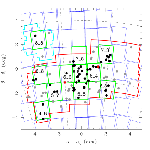
Figure 1: Distribution of the known ACs over the LMC (projected in the sky adopting $\alpha_{0}=81.0$ deg and $\delta_{0}=-69.0$ deg). Grey and black filled circles show the ACs observed by OGLE and those falling in the VMC tiles considered in this paper, respectively. The red filled circles represent the only two stars without a VMC counterpart within 1.0 arcsec (see text). Thin blue and thick green squares (distorted by the projection into the sky) show part of the VMC tiles in the LMC and the 11 tiles treated in this paper, respectively. The thick red and light blue lines show the areas covered by OGLE III and IV (released up to now), respectively.

2 Anomalous Cepheids in the VMC survey

ACs in the LMC were identified and characterized in the optical bands by Soszyński et al. (2008, and references therein) as part of the OGLE III project. For the LMC tile 8_8 (including the South Ecliptic Pole, or SEP) which lies outside the area imaged by OGLE III, we used results of an early release of stage IV of the OGLE survey (Soszyński et al., 2012). In these surveys, a total of 86 ACs were found (83 by OGLE III and 3 by OGLE IV), of which 66 are F and 20 are FO pulsators.

In this paper we present results for the ACs included in eleven“tiles” (1.5 sq. deg.) completely or nearly completely observed, processed and catalogued by the VMC survey as of March 2013, namely the tiles LMC 4_8, 5_3, 5_5, 5_7, 6_4, 6_5, 6_6, 6_8, 7_3, 7_5, and 8_8 (see Fig. 1). Tile LMC 6_6 is centred on the well known 30 Dor star forming region, tiles LMC 5_5, 6_4 and 6_5 are placed on the bar of the LMC, whereas the remaining tiles lie in less crowded regions of the galaxy. We note that tile LMC 8_8 encompasses the South Ecliptic Pole (SEP) which will be observed by the Gaia satellite during its commissioning phase (Lindegren & Perryman 1996; Lindegren 2010).

The general observing strategy of the VMC survey is described in detail in Paper I, whereas the procedures specifically applied to the variable stars can be found in Moretti et al. (2013). Here we only recall that to obtain well sampled light curves, the VMC $K_{\mathrm{s}}$-band time series observations were scheduled in 12 separate epochs distributed over ideally several consecutive months. The VMC data, processed through the pipeline (Irwin et al., 2004) of the VISTA Data Flow System (VDFS, Emerson et al., 2004) are in the VISTA photometric system (Vegamag=0). The time-series photometry used in this paper was retrieved from the VISTA Science Archive (VSA, Cross et al., 2012). For our analysis we used the VMC data acquired until the end of March 2013.

According to OGLE III/IV, 48 ACs are expected to lie in the 11 tiles analysed in this paper. Figure 1 and Tab. 1 show the distribution of such stars in the VMC tiles. The OGLE III and IV catalogues of ACs were cross-correlated against the VMC catalogue to obtain the $K_{\mathrm{s}}$ light curves for these variables.

All but one of the 48 ACs were found to have a counterpart in the VMC catalogue (see Tab. 2). The only object without VMC counterpart in the VSA within 3 arcsec (see Fig. 2) is OGLE-LMC-ACEP-024, which is expected to fall well within the tile LMC 6_4. This star has has a luminosity $I$=17.679 mag and $V$=17.986 mag and no remarks in the OGLEIII catalogue. There is a match if we enlarge the pairing radius to 5 arcsec, but the corresponding star is clearly too bright ($K_{\mathrm{s}}\sim$12.8 mag). An inspection of the VMC image reveals that the star is placed in the outskirts of the cluster NGC 1252, in a rather crowded region. This could explain the lack of a detection. For one of the objects with VMC identification, i.e. OGLE-LMC-ACEP-065 in tile LMC 6_6, the VSA database did not return any time-series data. This is likely because the star is located at the very edge of the frame, where the sensitivity is low and the target cannot be detected in the single epoch frames. Looking in more detail at this object on the VMC image (see Fig. 2), it appears that some crowding is present but the target should be easily detected at least in the neighbour tile LMC 5_6 which was not observed yet.

As shown in Tab. 2, the sample of ACs discussed here includes 36 F and 10 FO-mode pulsators. This sample represents more than 50% of the total number of ACs in the LMC. The VMC time-series $K_{\mathrm{s}}$ photometry for these 46 objects is provided in Table 3, which is published in its entirety in the on-line version of the paper.

Table 1: Number of Anomalous Cepheids in the 11 VMC tiles analyzed in this paper, according to OGLE III/IV.

Tile	RA (center)	DEC (center)	#ACs	Epochs	OGLE
LMC	J(2000)	J(2000)		(VMC)
4_8	06:06:32.95	$-$72:08:31.2	2	10	III
5_3	04:58:11.66	$-$70:35:28.0	4	11	III
5_5	05:24:30.34	$-$70:48:34.2	8	15	III
5_7	05:51:04.87	$-$70:47:31.2	3	8	III
6_4	05:12:55.80	$-$69:16:39.4	8	14	III
6_5	05:25:16.27	$-$69:21:08.3	10	9	III
6_6	05:37:40.01	$-$69:22:18.1	3	14	III
6_8	06:02:21.98	$-$69:14:42.4	2	14	III
7_3	05:02:55.20	$-$67:42:14.8	6	16	III
7_5	05:25:58.44	$-$67:53:42.0	1	14	III
8_8	05:59:23.14	$-$66:20:28.7	1	16	IV

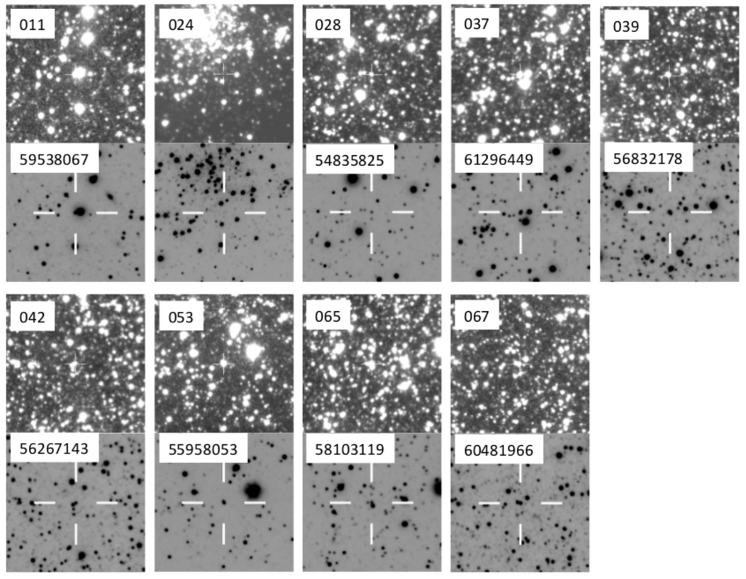
Figure 2: Sky pictures for nine problematic stars extracted from the VMC (lower panels) and the OGLE III (upper panels) archives. The target is identified in the single-epoch VMC images by a label showing the last 8 digits of the VMC identification. Similarly the corresponding OGLE III identification is reported with three digits (i.e. without the prefix “OGLE-LMC-AC-”).

Table 2: Cross-identification and main characteristics of the Anomalous Cepheids in the 11 “tiles” analysed in this paper. The columns report: 1) OGLE identification; 2) right ascension (OGLE); 3) declination (OGLE); 4) mode of pulsation; 5) period; 6) epoch of maximum light; 7) intensity–averaged $I$ magnitude (OGLE); 8) intensity–averaged $V$ magnitude (OGLE); 9) VMC identification; 10) VMC Tile; 11) Number of $K_{\mathrm{s}}$ epochs; 12) Notes on individual stars

ID	RA	DEC	M	Period	Epoch	$\langle I\rangle$	$\langle V\rangle$	VMC-ID	Tile	nEpochs	Notes
	J2000	J2000		d	d	mag	mag
(1)	(2)	(3)	(4)	(5)	(6)	(7)	(8)	(9)	(10)	(11)	(12)
OGLE-LMC-ACEP-035	5:18:22.19	$-$69:03:38.4	FO	0.446049	52115.88331	18.143	18.658	558355019633	6_4	14
OGLE-LMC-ACEP-013	4:59:56.62	$-$70:42:24.9	FO	0.500923	52166.70918	17.963	18.488	558359106778	5_3	11
OGLE-LMC-ACEP-043	5:24:35.40	$-$68:48:22.6	FO	0.50647	52167.59135	17.913	18.593	558356009732	6_5	9
OGLE-LMC-ACEP-028	5:13:10.02	$-$68:46:11.9	FO	0.599253	50457.56427	17.574	18.322	558354835825	6_4	14	a
OGLE-LMC-ACEP-068	5:51:09.02	$-$70:45:42.6	F	0.625645	52194.18981	18.265	18.809	558360489508	5_7	8
OGLE-LMC-ACEP-049	5:28:03.58	$-$69:39:15.2	F	0.644796	52167.32917	18.011	18.451	558356666394	6_5	9
OGLE-LMC-ACEP-071	5:54:43.24	$-$70:10:16.1	FO	0.676209	52187.35869	17.330	17.755	558360071488	5_7	8
OGLE-LMC-ACEP-045	5:26:24.68	$-$68:57:55.0	F	0.678431	52167.43289	18.325	18.976	558356105371	6_5	9
OGLE-LMC-ACEP-051	5:30:14.23	$-$68:42:31.1	F	0.708606	52167.2697	18.200	18.845	558355948009	6_5	9
OGLE-LMC-ACEP-023	5:07:52.42	$-$68:50:28.8	FO	0.723433	50726.2685	17.194	17.763	558354917807	6_4	14
OGLE-LMC-ACEP-034	5:17:11.15	$-$69:58:33.1	F	0.734298	52123.77557	17.874	18.474	558355708277	6_4	14
OGLE-LMC-ACEP-008	4:58:24.59	$-$71:05:11.5	FO	0.749068	52166.14121	17.300	17.911	558359341685	5_3	11
OGLE-LMC-ACEP-024	5:08:44.05	$-$68:46:01.2	F	0.794464	50726.76849	17.679	17.986	558354864345	6_4	0	b
OGLE-LMC-ACEP-009	4:58:51.29	$-$67:44:23.9	FO	0.80008	52166.34228	17.344	17.913	558351428166	7_3	16
OGLE-LMC-ACEP-081	6:09:38.40	$-$69:34:04.1	F	0.800838	52194.39949	17.917	18.504	558354433783	6_8	14
OGLE-LMC-ACEP-067	5:48:22.08	$-$70:45:49.3	F	0.820921	52168.84504	17.786	18.451	558360481966	5_7	7	c
OGLE-LMC-ACEP-010	4:59:00.10	$-$68:14:01.1	F	0.834201	52166.34125	18.068	18.723	558351741077	7_3	16
OGLE-LMC-ACEP-078	6:06:58.20	$-$72:52:08.7	FO	0.856556	52187.11324	16.979	17.417	558367620049	4_8	10
OGLE-LMC-ACEP-041	5:21:14.35	$-$70:29:39.5	F	0.878142	50831.14818	17.625	18.200	558361532603	5_5	15
OGLE-LMC-ACEP-063	5:37:54.39	$-$69:19:28.7	F	0.893031	52187.44348	18.013	18.756	558357554473	6_6	14
OGLE-LMC-ACEP-007	4:57:31.48	$-$70:15:53.6	F	0.896399	52166.18452	17.688	18.247	558358821009	5_3	11
OGLE-LMC-ACEP-017	5:02:03.13	$-$68:09:30.4	F	0.929995	52166.07849	17.585	18.190	558351666932	7_3	16
OGLE-LMC-ACEP-040	5:21:13.22	$-$70:34:20.7	F	0.960577	50831.32386	17.433	18.037	558361590075	5_5	15
OGLE-LMC-ACEP-054	5:31:06.72	$-$68:22:29.8	F	0.980222	52167.47834	17.901	18.798	558353586650	7_5	14
OGLE-LMC-ACEP-039	5:20:44.47	$-$69:47:46.5	F	0.992407	50455.25698	17.660	18.245	558356832178	6_5	9	c
OGLE-LMC-ACEP-011	4:59:38.09	$-$70:37:45.5	F	0.99859	51999.6182	17.671	18.254	558359538067	5_3	3	c
OGLE-LMC-ACEP-050	5:28:57.71	$-$70:07:15.5	FO	1.044691	50454.74962	16.609	17.049	558361189093	5_5	15
OGLE-LMC-ACEP-042	5:23:34.60	$-$69:10:58.2	F	1.079036	52167.36992	17.897	18.715	558356267143	6_5	5	c
LMC571.05.5070	6:01:41.77	$-$65:58:53.5	F	1.087061	55557.82471	17.181	17.686	558349409852	8_8	16
OGLE-LMC-ACEP-077	6:04:35.73	$-$71:40:35.8	F	1.122498	52187.66068	17.459	18.099	558367137280	4_8	10
OGLE-LMC-ACEP-056	5:31:49.45	$-$70:33:22.6	F	1.124003	52167.63676	17.284	17.877	558361558150	5_5	15
OGLE-LMC-ACEP-079	6:07:02.01	$-$69:31:55.2	F	1.15517	52176.92756	17.149	17.634	558354405855	6_8	14
OGLE-LMC-ACEP-037	5:19:16.67	$-$70:11:58.4	F	1.25774	52156.5207	17.132	17.743	558361296449	5_5	15	a
OGLE-LMC-ACEP-036	5:18:58.85	$-$69:26:47.8	F	1.257982	50455.67396	17.160	17.787	558355324744	6_4	23
OGLE-LMC-ACEP-052	5:31:01.53	$-$70:42:22.2	F	1.262555	52167.0715	17.008	17.577	558361664456	5_5	15
OGLE-LMC-ACEP-046	5:26:27.17	$-$69:58:57.0	F	1.263717	50454.39955	17.264	17.851	558356990050	6_5	9
OGLE-LMC-ACEP-021	5:06:37.49	$-$68:23:40.3	F	1.295843	50725.62518	17.188	17.827	558351789022	7_3	16
OGLE-LMC-ACEP-044	5:25:54.11	$-$69:26:52.9	F	1.308509	50455.10639	17.052	17.609	558356474792	6_5	9
OGLE-LMC-ACEP-032	5:15:56.13	$-$69:01:29.1	F	1.316022	50456.81167	17.167	17.780	558355007611	6_4	14
OGLE-LMC-ACEP-065	5:40:03.04	$-$70:04:47.8	F	1.3215432	50725.78028	17.041	17.508	558358103119	6_6	0	b
OGLE-LMC-ACEP-016	5:01:36.69	$-$67:51:33.1	F	1.54567	52166.4502	16.926	17.448	558351480147	7_3	16
OGLE-LMC-ACEP-048	5:27:12.12	$-$69:37:19.6	F	1.545893	50454.48193	16.718	17.324	558356636279	6_5	9
OGLE-LMC-ACEP-055	5:31:41.11	$-$68:44:37.7	F	1.606665	52189.7241	17.011	17.603	558357237330	6_6	14
OGLE-LMC-ACEP-057	5:31:49.88	$-$70:46:30.0	F	1.710008	52167.36219	16.813	17.455	558361710363	5_5	15
OGLE-LMC-ACEP-026	5:10:42.62	$-$68:48:19.6	F	1.738745	50457.22581	16.816	17.483	558354874727	6_4	14
OGLE-LMC-ACEP-053	5:31:06.20	$-$68:43:45.3	F	1.888099	52166.63019	16.738	17.299	558355958053	6_5	23	a
OGLE-LMC-ACEP-047	5:27:05.27	$-$71:23:33.4	F	2.177985	52166.33026	16.881	17.482	558362082677	5_5	15
OGLE-LMC-ACEP-014	5:00:08.26	$-$67:54:04.3	F	2.291346	52164.63844	16.639	17.241	558351518318	7_3	16
(a) stars showing significant blending but with useful light curves (see Figs.  2,  3, and Fig. 4)
(b) stars without $K_{\mathrm{s}}$ VMC data (see Fig. 2)
(c) stars showing significant blending and having unusable light curves (see Fig.  2 and  5)

Table 3: $K_{\mathrm{s}}$ time-series photometry of the ACs

HJD-2 400 000	$K_{\mathrm{s}}$	$\sigma_{K_{\mathrm{s}}}$
AC OGLE-LMC-ACEP-007
56267.81039	17.118	0.039
56316.64476	16.921	0.032
56318.55354	16.899	0.030
56322.63275	17.170	0.036
56328.57027	16.925	0.030
56334.54372	16.933	0.036
56341.53132	17.200	0.042
56347.56046	17.036	0.032
56371.53252	16.923	0.034
56372.51981	16.952	0.034
56375.52238	17.112	0.034

Table 3 is published in its entirety only in the electronic edition of the journal. A portion is shown here for guidance regarding its form and content.

Periods and Epochs of maximum light available from the OGLE III catalogue were used to fold the $K_{\mathrm{s}}$–band light curves produced by the VMC observations. The OGLE IV catalogue provides only the period for the AC LMC571.05.5070, hence we obtained the Epoch of maximum from the analysis of the star $V$-band light curve. The $K_{\mathrm{s}}$–band light curves for a sample of 42 ACs with useful light curves are shown in Figs. 3 and 4. Apart from a few cases these light curves are generally well sampled and nicely shaped. Intensity-averaged $\langle K_{\mathrm{s}}\rangle$ magnitudes were derived from the light curves simply using custom software written in C, that performs a spline interpolation to the data with no need of using templates. Some evidently discrepant data points in the light curves were excluded from the fit but were plotted in the figure for completeness (note that most of these “bad” data points belong to observations collected during nights that did not strictly meet the VMC quality criteria). The final spline fit to the data is shown by a solid line in Figs.  3 and 4. Final $\langle K_{\mathrm{s}}\rangle$ magnitudes are provided in Table 4.

Four objects in our sample were excluded, namely: OGLE-LMC-ACEP-011, 039, 042, 067. Their light curves are displayed in Fig. 5, whereas their finding charts are shown in Fig. 2. A quick analysis of the finding charts reveals that all these stars have significant problems of crowding/blending (particularly, star 011).

Table 4: Results for the 42 Anomalous Cepheids with useful light curves analysed in this paper. The columns report: 1) OGLE identification; 2) mode of pulsation; 3) period; 4) intensity–averaged $K_{\mathrm{s}}$ magnitude; 5) uncertainty on the $\langle K_{\mathrm{s}}\rangle$; 6) peak–to–peak amplitude in $K_{\mathrm{s}}$ ; 7) adopted reddening; 8) correction in magnitude due to the deprojection.

ID	M	Period	$\langle K_{\mathrm{s}}\rangle$	$\sigma_{\langle K_{\mathrm{s}}\rangle}$	$Amp(K_{\mathrm{s}})$	$E($V-I$)$	$\Delta$
		d	mag	mag	mag	mag	mag
(1)	(2)	(3)	(4)	(5)	(6)	(7)	(8)
OGLE-LMC-ACEP-035	FO	0.446049	17.585	0.026	0.17	0.07	0.026
OGLE-LMC-ACEP-013	FO	0.500923	17.334	0.033	0.06	0.03	0.068
OGLE-LMC-ACEP-043	FO	0.50647	17.186	0.051	0.08	0.09	0.013
OGLE-LMC-ACEP-028	FO	0.599253	16.399	0.010	0.08	0.06	0.040
OGLE-LMC-ACEP-068	F	0.625645	17.490	0.049	0.26	0.06	$-$0.042
OGLE-LMC-ACEP-049	F	0.644796	17.412	0.028	0.12	0.04	0.003
OGLE-LMC-ACEP-071	FO	0.676209	16.790	0.015	0.12	0.07	$-$0.053
OGLE-LMC-ACEP-045	F	0.678431	17.499	0.045	0.33	0.11	0.008
OGLE-LMC-ACEP-051	F	0.708606	17.437	0.023	0.17	0.10	0.000
OGLE-LMC-ACEP-023	FO	0.723433	16.444	0.005	0.13	0.08	0.052
OGLE-LMC-ACEP-034	F	0.734298	17.186	0.022	0.26	0.13	0.028
OGLE-LMC-ACEP-008	FO	0.749068	16.567	0.007	0.14	0.08	0.072
OGLE-LMC-ACEP-009	FO	0.80008	16.575	0.014	0.16	0.06	0.081
OGLE-LMC-ACEP-081	F	0.800838	17.147	0.017	0.13	0.07	$-$0.090
OGLE-LMC-ACEP-010	F	0.834201	17.225	0.015	0.35	0.11	0.077
OGLE-LMC-ACEP-078	FO	0.856556	16.372	0.018	0.16	0.09	$-$0.057
OGLE-LMC-ACEP-041	F	0.878142	16.790	0.020	0.17	0.09	0.021
OGLE-LMC-ACEP-063	F	0.893031	16.990	0.026	0.20	0.18	$-$0.020
OGLE-LMC-ACEP-007	F	0.896399	17.002	0.020	0.25	0.06	0.073
OGLE-LMC-ACEP-017	F	0.929995	16.810	0.015	0.25	0.06	0.070
OGLE-LMC-ACEP-040	F	0.960577	16.644	0.012	0.18	0.09	0.021
OGLE-LMC-ACEP-054	F	0.980222	16.781	0.029	0.17	0.26	$-$0.000
OGLE-LMC-ACEP-050	FO	1.044691	16.016	0.011	0.14	0.07	0.003
LMC571.05.5070	F	1.087061	16.479	0.007	0.25	0.08	$-$0.072
OGLE-LMC-ACEP-077	F	1.122498	16.608	0.002	0.08	0.07	$-$0.062
OGLE-LMC-ACEP-056	F	1.124003	16.527	0.019	0.19	0.06	$-$0.002
OGLE-LMC-ACEP-079	F	1.15517	16.471	0.013	0.26	0.05	$-$0.085
OGLE-LMC-ACEP-037	F	1.25774	15.332	0.007	0.04	0.08	0.024
OGLE-LMC-ACEP-036	F	1.257982	16.388	0.022	0.13	0.08	0.023
OGLE-LMC-ACEP-052	F	1.262555	16.316	0.011	0.27	0.07	0.001
OGLE-LMC-ACEP-046	F	1.263717	16.570	0.016	0.35	0.03	0.008
OGLE-LMC-ACEP-021	F	1.295843	16.377	0.027	0.20	0.07	0.058
OGLE-LMC-ACEP-044	F	1.308509	16.380	0.024	0.48	0.06	0.007
OGLE-LMC-ACEP-032	F	1.316022	16.360	0.010	0.20	0.06	0.032
OGLE-LMC-ACEP-016	F	1.54567	16.261	0.006	0.30	0.05	0.073
OGLE-LMC-ACEP-048	F	1.545893	15.958	0.018	0.25	0.07	0.005
OGLE-LMC-ACEP-055	F	1.606665	16.188	0.010	0.26	0.08	$-$0.003
OGLE-LMC-ACEP-057	F	1.710008	16.006	0.017	0.43	0.07	$-$0.001
OGLE-LMC-ACEP-026	F	1.738745	15.932	0.011	0.27	0.08	0.046
OGLE-LMC-ACEP-053	F	1.888099	15.682	0.011	0.26	0.11	$-$0.002
OGLE-LMC-ACEP-047	F	2.177985	16.181	0.009	0.31	0.07	0.012
OGLE-LMC-ACEP-014	F	2.291346	15.862	0.008	0.29	0.04	0.076

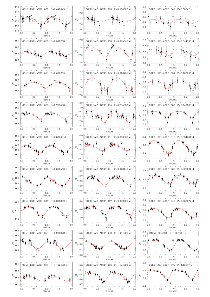
Figure 3: $K_{\mathrm{s}}$–band light curves for 27 of the 42 ACs with usable data discussed in this paper. Stars are displayed in order of increasing period. Solid lines represent spline best-fits to the data (see text). In each panel we report OGLE’s identification number and period.

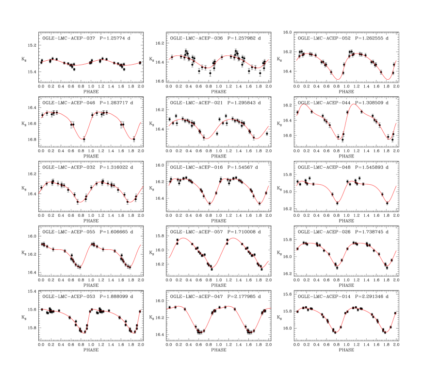
Figure 4: As in Fig. 3 but for the remaining 15 ACs of our sample.

It is important to remember that all the $K_{\mathrm{s}}$ photometry presented in this paper is in the VISTA system. To make it easy to compare our results with the widely used 2MASS system, we note that the two systems are very close to each other. In particular, the VMC $K_{\mathrm{s}}$ magnitude depends only mildly on the ($J$$-$$K_{\mathrm{s}}$) colour. Indeed, the empirical results available to date show that: ($J$$-$$K_{\mathrm{s}}$)(2MASS)=1.081($J$-$K_{\mathrm{s}}$)(VISTA) and $K_{\mathrm{s}}$(2MASS)=$K_{\mathrm{s}}$(VISTA)$-$0.011($J$-$K_{\mathrm{s}}$)(VISTA). Unfortunately, for the majority of our targets we only have a few $J$ measurements (4 phase points), hence a star-by-star correction based on the $(\langle J\rangle-\langle K_{\mathrm{s}}\rangle)$ colour is likely to introduce larger errors than the correction itself. Furthermore, since the measured ($\langle$$J$ $\rangle$$-$$\langle$ $K_{\mathrm{s}}$$\rangle$) of our AC sample typically ranges from 0.2 to 0.5 mag, the average correction over the 42 ACs considered here, is as small as $-3.0\pm$1.0 mmag and can be safely neglected. In conclusion, for ACs, as well as for CCs (see Ripepi et al., 2012b), to a very good approximation, the VISTA and 2MASS $K_{\mathrm{s}}$ can be considered equivalent.

3 Optical Period-Luminosity, Period-Luminosity-Colour and Period-Wesenheit relations

Before presenting the results in the NIR bands, in this section we derive the coefficients of the optical ($V,I$) $P$–$L$, $P$–$L$–$C$ and Wesenheit–$W(V,I)$ relations, based on the OGLE data, since they are still lacking in the literature. Indeed, neither Soszyński et al. (2008) nor Fiorentino & Monelli (2012) published these relations, although they showed them in some figures. In this case we have used the whole sample of ACs detected in the LMC by the OGLE III/IV surveys.

The first step is to correct for reddening, which unfortunately is rather variable in the LMC, hence needs to be evaluated locally. To this aim, we adopted the recent estimates by Haschke, Grebel & Duffau (2011). Individual $E$($V$$-$$I$) reddening values for the 42 ACs with useful VMC data are reported in column 7 of Table 4. In Sect. 5 we will check the soundness of these reddening values.

The second step consists of accounting for the inclination of the LMC disc-like structure by de-projecting each AC with respect to the LMC centre. We followed the procedure outlined in van der Marel & Cioni (2001) and adopted their values of the LMC centre, inclination, and position angle of the line of nodes (see column 8 of Tab. 4).

Finally, we performed least-squares fits to the data of F and FO-mode variables separately, adopting equations of the form Mag=$\alpha+\beta$ log$P$, with Mag$=V,I$. The best-fitting relationships are shown in the left panels of Fig. 6, their coefficients are provided in the first portion of Table 5. We note that in all panels of this figure, the stars plotted with crosses and open circles were rejected from the fit because they are 2.5-3 $\sigma$ off the regression line. In particular, the three objects with the longest periods, namely OGLE-LMC-ACEP-014, 033, 047 (crosses in Fig. 6) are likely not ACs but rather members of some different variable classes such as BL Herculis stars. Indeed, looking at Fig. 1 in Soszyński et al. (2008) it is clear that some confusion can be possible between ACs and BL Her pulsators at the periods of interest. Additional stars that were not used in at least one of the regressions are OGLE-LMC-ACEP-022, 024, 028, 042, 059, 083. All these objects, with the possible exception of 022, show some observational problems. In particular, the stars 024, 042, 028 will be discussed in detail in the next section, since they are problematic also in the VMC data (see Fig. 2). As for the remaining three, we inspected the OGLE images and light curves, finding that in the case of the star 083 there is a strong background variation close to the object (possibly close to an edge of the CCD) and the star light curves appear to be rather noisy. Stars 022 and 059 are surrounded by a number of close companions and both of them show a rather noisy light curve, especially star 059, that has also a large $(V-I)$ colour ($>$1.2 mag).

Figure 5: Light curves for four problematic stars (see text).

In addition to the $V,I$ $P$–$L$ relations we can also derive the $P$–$W$ and $P$–$L$–$C$ relations. The advantages of using these relations instead of a simple $P$–$L$ have been widely discussed in the literature (see e.g. Marconi et al., 2004, in the case of ACs). Briefly, these relations include a colour term with a coefficient that, in the case of the $P$–$L$–$C$ relation, takes into account the colour distribution of the variable stars within the instability strip, whereas in the case of the Wesenheit function corresponds to the ratio between total-to-selective extinction in the filter pair (Madore, 1982; Caputo, Marconi & Musella, 2000), thus making the Wesenheit relations reddening free by definition. We expect these relations to have much smaller dispersion than a simple $P$–$L$ relation, even if the scatter reduction for ACs is not as significant as in the case of CCs (see e.g. Marconi, Musella, & Fiorentino, 2005; Marconi et al., 2004). In fact, for CCs a strict Mass-Luminosity ($ML$) relation is predicted to exist by stellar evolution computations for He burning intermediate mass stars, which makes the $P$–$L$–$C$ a relation holding for each individual pulsator (see e.g. Caputo, Marconi & Musella, 2000, for details). Unfortunately, the ACs are not characterized by such a strict $ML$ relation, thus the resulting $P$–$L$–$C$ and $P$–$W$ relations include the possible effect of mass differences at fixed luminosity level.
The $P$–$W$ and $P$–$L$–$C$ relations are usually calculated using the $(V-I)$ colour. The coefficients of the relations derived with this procedure for the LMC ACs are provided in the lower portions of Table 5. The relations are shown in the right panels of Fig. 6. The dispersion of the $P$–$W$ and $P$–$L$–$C$ relations is of the order of $\sim$ 0.15 mag (see Tab. 5), hence smaller than for the $P$–$L$ relation but larger than in the case of CCs (see e.g. Soszyński et al., 2008, who found a $\sigma$=0.08 mag for the $P$–$W(V,I)$ relation).

Table 5: Optical $P$–$L$, $P$–$W$ and $P$–$L$–$C$ relations for F and FO Anomalous Cepheids. The Wesenheit function is defined as: $W(V,I)=V-2.54(V-I)$.

mode	$\alpha$	$\sigma_{\alpha}$	$\beta$	$\sigma_{\beta}$	$\gamma$	$\sigma_{\gamma}$	r.m.s.
$V^{0}$=$\alpha$+$\beta$ log$P$
F	17.90	0.03	$-$3.21	0.21			0.20
FO	17.20	0.09	$-$3.14	0.37			0.23
$I^{0}$=$\alpha$+$\beta$ log$P$
F	17.38	0.02	$-$3.22	0.19			0.18
FO	16.74	0.06	$-$3.23	0.25			0.16
$W(V,I)=\alpha+\beta$ log$P$
F	16.59	0.02	$-$3.41	0.16			0.15
FO	16.05	0.05	$-$3.44	0.22			0.13
$V^{0}=\alpha+\beta$ log$P$$+\gamma($V-I$)^{0}$
F	16.71	0.09	$-$3.40	0.14	2.34	0.16	0.14
FO	16.24	0.13	$-$3.34	0.18	2.14	0.28	0.12

Table 6: NIR $P$–$L$ and $P$–$W$ relations for F and FO-mode Anomalous Cepheids. The Wesenheit function is defined as: $W(V,K)$=$K_{\mathrm{s}}$$-$0.13 ($V$$-$$K_{\mathrm{s}}$). Note that all the results are in the VISTA photometric system.

mode	$\alpha$	$\sigma_{\alpha}$	$\beta$	$\sigma_{\beta}$	$\gamma$	$\sigma_{\gamma}$	r.m.s.
$K_{\mathrm{s}}^{0}$=$\alpha$+$\beta$ log$P$
F	16.74	0.02	$-$3.54	0.15			0.10
FO	16.06	0.07	$-$4.18	0.33			0.10
$W(V,K_{\mathrm{s}})=\alpha+\beta$ log$P$
F	16.58	0.02	$-$3.58	0.15			0.10
F	15.93	0.07	$-$4.14	0.33			0.10

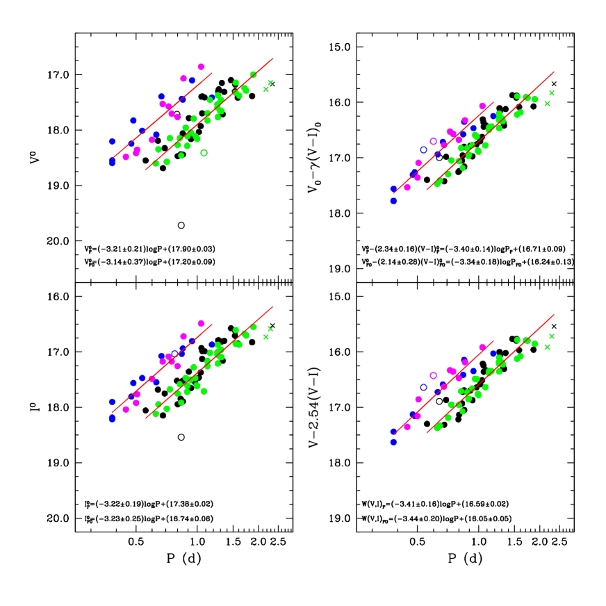
Figure 6: Optical $P$–$L$, $P$–$W$ and $P$–$L$–$C$ relations for F and FO Anomalous Cepheids. The Wesenheit function is defined as: $W(V,I)=V-2.54(V-I)$. In each panel, green and black filled circles are OGLE F pulsators, blue and magenta filled circles are OGLE FO pulsators, with (in green and magenta) or without (in black and blue) VMC $K_{\mathrm{s}}$ measurements. Empty circles and crosses mark pulsators that were discarded in the derivation of the $P$–$L$ and $P$–$W$ (and the optical $P$–$L$–$C$) relations. In particular, the three stars with longest periods (crosses) likely are not ACs and rather belong to a different type of variability. In all panels, the red lines show the best-fits to the data, with the corresponding relationships labelled at the bottom.

4 $K_{\mathrm{s}}$-band Period-Luminosity and Period-Wesenheit relations

By analogy to the optical $V,I$ bands, we can calculate the $P$–$L$, and $P$–$W$ relationships in the $K_{\mathrm{s}}$-band. Our sample consist of 32 F-mode and 10 FO-mode ACs that are sufficient to provide statistically meaningful $P$–$L$ and $P$–$W$ relations. For both modes of pulsation our sample maps the whole range of periods covered by the LMC ACs, as shown in Fig. 6, where we have plotted in green and magenta colours the F and FO-mode objects observed by VMC, respectively. The $K_{\mathrm{s}}$-band $P$–$L$ and $P$–$W$ relations obtained are displayed in Fig. 7, whereas their coefficients are summarized in Tab. 6. Three F-mode and one FO-mode stars were excluded from the fit because they are more than 2$\sigma$ off the regression lines. The stars OGLE-LMC-ACEP-037 and 028, a F and FO-mode pulsators respectively, are shown with empty circles in Fig. 7. They have rather “normal” light curves, but at least the star 037 is clearly blended (see Fig. 2). The star 028 also exhibit an unusual colour (see Sect. 5 and Fig. 9) and we hypothesize that it may be blended, however, we do not have enough resolution to detect the contaminant star. The two additional F-Mode ACs excluded from the fit (namely, OGLE-LMC-ACEP-014 and OGLE-LMC-ACEP-047, shown as crosses in Fig. 7) are the stars with the longest periods. They were excluded also in the optical analysis as we suspect they could possibly belong to a separate class of variables. We note that, as for CCs, moving to the NIR the dispersion of the AC $P$–$L$ and $W(V,K_{\mathrm{s}})$ relations decreases. We also made an attempt to calculate $P$–$L$–$C$ relations in the form $K_{\mathrm{s}}^{0}$=$f({\rm log}P,(V-K_{\mathrm{s}})_{0})$, but the colour term coefficient turned out to be statistically equal to zero. This is not very surprising given the relatively small number of pulsators and the almost identical dispersions of the $P$–$L$ and $P$–$W$ relations. Hence, according to this dataset, in the NIR filters it seems that there is no great advantage in using the AC $P$–$L$–$C$ or pseudo $P$–$L$–$C$ relations instead of the $P$–$L$.

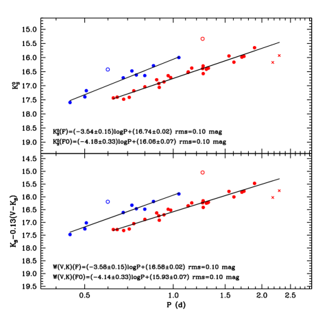
Figure 7: Top panel: $K_{\mathrm{s}}$-band $P$–$L$ relation for F and FO-mode ACs (red and blue symbols, respectively). Filled circles show the objects used for the least square fits. Stars marked by open circles and crosses were discarded (see text for detail). The solid lines is the least squares fit to the data. Bottom panel: as for the top panel but for the Wesenheit function, which is defined as labelled in the figure.

5 Comparison with literature and application to real cases

To compare our $P$–$L$s for ACs with the relations available in the literature, we first need to set the absolute zero points. This can be done by assuming a proper value for the distance to the host galaxy, the LMC. We have adopted our own evaluation based on the absolute calibrations of the $P$–$L$, $P$–$L$–$C$ and $W(V,K_{\mathrm{s}})$ relations for CCs in the LMC presented in Ripepi et al. (2012b). In that paper we used the trigonometric parallaxes of Galactic Cepheids as well as Baade-Wesselink measurements of Cepheids in the LMC to evaluate $DM_{\rm LMC}^{0}=18.46\pm 0.03$ mag (see Ripepi et al., 2012b, for full details.). This distance modulus is in very good agreement with current literature estimates for the distance to the LMC as nicely reviewed by Walker (2012), and with the very recent and precise value by Pietrzyński et al. (2013), based on eclipsing binaries. Results of this comparison in the optical are summarized in the first part of Tab. 7 and graphically shown in Fig. 8 for the $P$–$L$ and the Wesenheit relations, respectively.

The upper panel of Fig. 8 shows the comparison of our $P$–$L$s with the relations derived empirically by Pritzl et al. (2002) and Marconi et al. (2004) on the basis of a few tens of ACs belonging to a number of dwarf Spheroidal galaxies (dSph) orbiting the Milky Way and M31 spirals. There is a clear disagreement between our results and the literature. This is likely due to a number of reasons: i) the very different coverage of the AC instability strip, which is much more uniformly and completely covered in the LMC sample; ii) at shorter periods (P$\sim$0.4-0.5 d) it is easy to confuse F– and FO–mode pulsators, especially in the dSphs where samples are generally rather small; iii) the non-homogeneous dSph sample. A better agreement, at least for the F-mode pulsators, can be seen in the bottom panel of Fig. 8, where we compare our $W(V,I)$ function with those by Marconi et al. (2004), the only published relation to date. The better agreement in this case is probably due to the much lower dependence of the $W(V,I)$ with respect to the $P$–$L$ on the way the pulsators populate the instability strip.

Marconi et al. (2004) also published mass-dependent, $P$–$L$–$C$ and Wesenheit (the latter only for F-mode pulsators) relations for ACs calculated on the basis of non–linear, non–local time-dependent convective pulsation models. The lower portion of Tab. 7 reports the comparison between Marconi et al. (2004) theoretical models and our results. There is good agreement for the slope of the $P$–$W(V,I)$ relations, however, our zero point implies a stellar mass of $M\sim 1.3M_{\odot}$, at the lower end of the allowed range for ACs.

As for the $P$–$L$–$C$, both the slopes and the zero point disagree by more than 1 $\sigma$. We do not have a clear explanation for these discrepancies, however, if the reddening values we have adopted for the ACs are correct, the disagreement could in principle be related to uncertainties in the theoretical colour-temperature relations.

There are no other empirical NIR relations in the literature we are aware of, hence we can compare our results only with the colour-colour and the $P$–$W(V,K_{\mathrm{s}})$ relations derived by Marconi et al. (2004) from the theory of stellar pulsation. The top panel of Fig. 9 shows this comparison for the 42 pulsators analysed in this paper in the $(V-I)_{0}$$-$$(V-K_{\mathrm{s}})_{0}$ plane. Overall the agreement is very satisfactory. The residual discrepancy can be minimized by a difference in the adopted reddening of only $\langle\Delta E(V-I)\rangle=-0.01\pm 0.02$ mag. This is a confirmation that the reddening values adopted in this paper are well–established. An inspection of the figure confirms that the two stars OGLE-LMC-ACEP-037 and 028 (empty circles), previously excluded from the $P$–$L$ and $P$–$W$ derivation, are highly deviant also in the colour-colour plane. In addition, we find a third discrepant star in this plane: OGLE-LMC-ACEP-053 (empty star). Also this object is clearly blended (see Fig. 2), so that its strange position in the colour-colour plane can be easily explained. Since this AC shows a rather normal light curve and it is not deviant e.g. in the $P$–$L$ relation, we conclude that its photometry is only mildly affected by the blending star.

The lower panel of Fig. 9 shows the comparison between our F-mode $P$–$W(V,K_{\mathrm{s}})$ relation and theoretical predictions (not available for FO-mode pulsators), for three different choices of the AC mass encompassing approximately the whole range of allowed values for this parameter, namely $M=1.3,1.6$ and $1.9M_{\odot}$. There is a good agreement for the slope of the $P$–$W(V,K_{\mathrm{s}})$ relations, whereas, as already found for the optical $P$–$W(V,I)$, our zero-point seems to favor the smallest value of $M=1.3M_{\odot}$, for the mass.

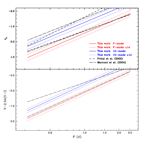
Figure 8: Comparison between the optical $P$–$L$ (top panel) and $P$–$W(V,I)$ relations (bottom panel) for F and FO-mode ACs derived in this paper with the literature results.

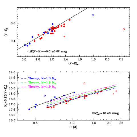
Figure 9: Top panel: $(V-I)_{0}$ versus $(V-K_{\mathrm{s}})_{0}$ plot for the F-mode ACs analysed in this paper. Symbols are as in Fig. 7. The solid line represents the theoretical relation by Marconi et al. (2004). The theoretical $(V-K_{\mathrm{s}})_{0}$ was converted to the 2MASS system using the relations in Tab. 7. Bottom panel: comparison between the observed Wesenheit $K_{\mathrm{s}}$-band relation for F-mode (solid line; note that the FO-mode relation is shown, too) and the predictions by Marconi et al. (2004) for three different choices of the pulsator mass (dashed lines, see labels).

Table 7: Literature values for the coefficients of the $P$–$L$, $P$–$W$ and $P$–$L$–$C$ relations, for F and FO Anomalous Cepheids. The Wesenheit functions are defined as: $W(V,I)=V-2.54(V-I)$ and $W(V,K_{\mathrm{s}})=K_{\mathrm{s}}-0.13(V-K_{\mathrm{s}})$. In the $K_{\mathrm{s}}$, the photometry of previous studies was converted to the 2MASS system, for consistency with our results (see Section 2).

mode	$\alpha$	$\sigma_{\alpha}$	$\beta$	$\sigma_{\beta}$	$\gamma$	$\sigma_{\gamma}$	r.m.s.	source
$M_{V}^{0}$=$\alpha$+$\beta$ log$P$
F	$-0.56$	0.04	$-3.21$	0.21			0.20	This paper
F	$-0.71$	0.03	$-2.64$	0.17				Pritzl et al. (2002)
F	$-0.70$	0.14	$-2.73$				0.14	Marconi et al. (2004)(a)
FO	$-1.26$	0.09	$-3.14$	0.37			0.23	This paper
FO	$-1.61$	0.07	$-3.74$	0.20			0.25	Pritzl et al. (2002)
FO	$-1.58$	0.25	$-2.95$				0.25	Marconi et al. (2004)(a)
$W(V,I)=\alpha+\beta$ log$P$
F	$-1.87$	0.04	$-3.41$	0.16			0.15	This paper
F	$-1.93$	0.20	$-3.34$				0.20	Marconi et al. (2004)(a)
F	$-1.74-1.83$$\log{M}$	0.20	$-3.34$				0.20	Marconi et al. (2004)(b)
FO	$-2.41$	0.06	$-3.44$	0.22			0.13	This paper
FO	$-2.52$	0.20	$-2.51$				0.20	Marconi et al. (2004)(a)
$M_{V}^{0}=\alpha+\beta$ log$P+\gamma(V-I)_{0}$
F	$-1.75$	0.09	$-3.40$	0.14	2.34	0.16	0.14	This paper
F	$-1.83-1.89$$\log{M}$		$-2.93$		2.73		0.01	Marconi et al. (2004)(b)
FO	$-2.22$	0.13	$-3.34$	0.18	2.14	0.28	0.12	This paper
FO	$-2.24-1.73$$\log{M}$		$-3.09$		2.67		0.01	Marconi et al. (2004)(b)
$K_{\mathrm{s}}=\alpha+\beta$ log$P$
F	$-1.72$	0.04	$-3.54$	0.15			0.10	This paper
FO	$-2.40$	0.07	$-4.18$	0.33			0.10	This paper
$W(V,K_{\mathrm{s}})=\alpha+\beta$ log$P$
F	$-1.88$	0.04	$-3.58$	0.15			0.10	This paper
F	$-1.71-1.83$$\log{M}$		$-2.93$				0.04	Marconi et al. (2004)(b,c)
FO	$-2.53$	0.07	$-4.14$	0.33			0.10	This paper
(a) Empirical
(b) Theoretical, the value of the mass ranges from 1.3 to 1.9 $M_{\odot}$
(c) Models transformed to the Johnson system: for ACs $K$(Johnson) $\approx K$(SAAO)
(see Bessell & Brett, 1988). $K_{\mathrm{s}}$(2MASS)$=K$(SAAO)$+0.02(J-K)$(SAAO)$-0.025$ (Carpenter, 2001)

5.1 Application of the optical $P$–$W$ relation

In the previous sections we have shown that the $P-W(V,I)$ relation is likely the best tool we have to use the ACs as standard candles. Indeed, the $P-W(V,I)$ relation does not depend on the reddening and on how the pulsators populate the instability strip. This obviously holds also for the $P-W(V,K_{\mathrm{s}})$. However, at present the lack of NIR observations of ACs in other galaxies limits severely the use of this relation. On the contrary, $V,I$ data are available for a significant number of ACs belonging to a few dwarf galaxies in the Local Group that can be used to verify the ability of our $P-W(V,I)$ to estimate the distance to the host systems by comparing AC-based and RR Lyrae-based distance determinations.

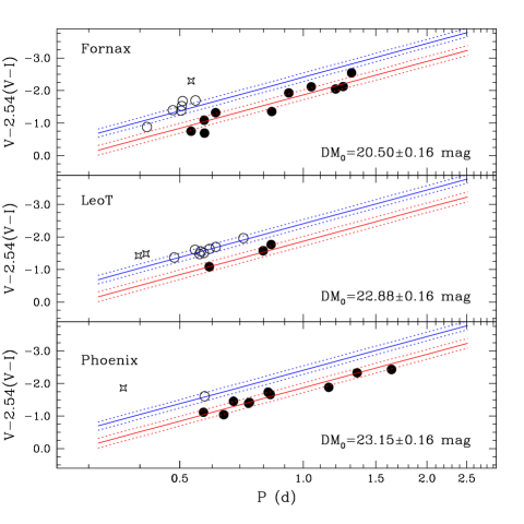
Figure 10: Optical $P-W(V,I)$ relations for ACs in a number of Local Group dwarf galaxies in comparison with the results obtained in this paper. F and FO-mode ACs are marked by filled and empty circles, respectively; starred symbols refer to objects with uncertain classification that were not used in calculating the distances. Red and blue lines show present work $P-W(V,I)$ for F and FO-mode ACs, respectively. True distance moduli estimated from these relations are labelled.

To our knowledge, there are only three dwarf galaxies with a significant number of ACs measured in the $V,I$ bands, namely, Fornax (Bersier & Wood, 2002), Leo T (Clementini et al., 2012), and Phoenix (Gallart et al., 2004). There is no clear separation between F and FO-mode pulsators in these galaxies (see Pritzl et al., 2002; Marconi et al., 2004), hence we used our own $P$–$W$ relation to perform a tentative subdivision of the samples into the two modes. The result of the overall procedure is shown in Fig. 10, where the different panels report the results for the three afore-mentioned galaxies. The distance moduli labelled in the figures were obtained trying to adjust simultaneously F-mode and FO-mode pulsators, and weighting the results to take into account the number of pulsators in each of the two modes. Errors on the derived distances are dominated by the dispersion of the LMC $P-W(V,I)$, whereas the uncertainty of the LMC distance is significantly smaller.

In Table 8 we compare the distances obtained from the ACs and literature values based on RR Lyrae or other distance indicators. Our distance modulus for the Fornax dSph is systematically smaller than all the other determinations, but still in agreement with most of them within 1$\sigma$. On the contrary, the agreement is rather good for Leo T and excellent for Phoenix. On this basis, it is not easy to explain why we find such shorter distances for Fornax dSph. New observations, including the complete sample of ACs belonging to this very large galaxy are needed to clarify this point.

Concluding, the $P-W(V,I)$ derived in this paper is a reliable tool for the determination of the distance to galaxies hosting significant samples of ACs.

Table 8: Comparison between distances derived from the ACs in this paper and the literature values for the Fornax, Leo T, and Phoenix Local Group dwarf.

method	$DM_{0}$	Reference
Fornax: $DM_{0}$(ACs)=20.50$\pm$0.16 mag (15 ACs)
TRGB	20.76$\pm$0.20	(1)
Red Clump	20.66	(2)
TRGB	20.65$\pm$0.11	(2)
Red Clump	20.86$\pm$0.01	(3)
RR Lyrae	20.72$\pm$0.10	(4)
TRGB	20.75$\pm$0.19	(5)
HB	20.70$\pm$0.12	(6)
TRGB	20.84$\pm$0.18	(7)
RR Lyrae	20.66$\pm$0.07	(8)
Leo T: $DM_{0}$(ACs)=22.88$\pm$0.16 mag (11 ACs)
TRGB	23.1$\pm$0.2	(9)
SFH-Fitting	23.05	(10)
RR Lyrae	23.06$\pm$0.15	(11)
Phoenix: $DM_{0}$(ACs)=23.15$\pm$0.16 mag (11 ACs)
TRGB	23.0$\pm$0.1	(12)
TRGB	23.21$\pm$0.08	(13)
TRGB	23.11	(14)
Mira	23.10$\pm$0.18	(15)
TRGB	23.09$\pm$0.10	(16)
(1) Buonanno et al. (1999); (2) Bersier (2000);
(3) Pietrzyński, Gieren, & Udalski (2003); (4) Greco et al. (2005);
(5) Gullieuszik et al. (2007); (6) Rizzi et al. (2006);
(7) Pietrzyński et al. (2009); (8) Greco et al. (2009);
(9) Irwin et al. (2007); (10) Weisz et al. (2012);
(11) Clementini et al. (2012);
(12) Martínez-Delgado, Gallart & Aparicio (1999);
(13) Held, Saviane & Momany (1999);
(14) Holtzman, Smith & Grillmair (2000);
(15) Menzies et al. (2008); (16) Hidalgo et al. (2009);

6 Summary and Conclusions

We have presented the first light curves in the NIR $K_{\mathrm{s}}$-band for Anomalous Cepheids. In particular, our sample consists of 46 AC pulsators (36 F-mode and 10 FO-mode) located in the LMC and observed by the VMC survey. Our light curves are well sampled with the number of epochs ranging from 8 to 23. In spite of the faintness of the LMC ACs, these data allowed us to obtain very precise mean $K_{\mathrm{s}}$ magnitudes for the pulsators, with average errors of the order of 0.01 mag.

The $\langle K_{\mathrm{s}}\rangle$ magnitudes were used to build the first $P$–$L$ and $P$–$W$ relations in the NIR for F and FO-mode ACs. At the same time we exploited the OGLE optical ($V,I$) data for ACs to construct accurate optical $P$–$L$, $P$–$L$–$C$ and $P$–$W$ relations both for F- and FO-mode ACs. These relations were obtained for the first time from a sample of pulsators covering in a uniform and complete way the AC instability strip.

The application of the $P$–$W(V,I)$ relation to three dwarf galaxies hosting significant populations of ACs, revealed that this relation is a valuable tool for deriving distances within the Local Group. Due to the lower dispersion, we expect that the $P$–$W(V,K_{\mathrm{s}})$ first derived in this paper will become an even better tool for measuring distances to galaxies hosting ACs. More NIR ($K_{\mathrm{s}}$-band in particular) data for ACs in other Local Group galaxies are needed to properly exploit the properties of the $P$–$W(V,K_{\mathrm{s}})$ relation.

References

- Bekki & Chiba (2007) Bekki K., Chiba M., 2007, MNRAS, 381, L16
- Bersier (2000) Bersier, D., 2000, ApJ, 534, L23
- Bersier & Wood (2002) Bersier D., & Wood P. R. 2002, AJ, 123, 840
- Bessell & Brett (1988) Bessell, M. S., Brett, J. M., 1988, PASP, 100, 1134
- Brocato et al. (2004) Brocato E., Caputo F., Castellani V., Marconi M., Musella I., 2004, AJ, 128, 1597
- Buonanno et al. (1999) Buonanno R., Corsi C.E., Castellani M., Marconi G., Fusi Pecci F., Zinn R., 1999, AJ, 118, 1671
- Caputo (1998) Caputo F. 1998, A&ARv, 9, 33
- Caputo, Marconi & Musella (2000) Caputo F., Marconi M., Musella I., 2000, A&A, 354, 610
- Caputo et al. (2004) Caputo F., Castellani V., Degl’Innocenti S., Fiorentino G., Marconi M. 2004, A&A, 424, 927
- Carpenter (2001) Carpenter J.M., 2001, AJ, 121, 2851
- Cioni et al. (2011) Cioni M.-R. L., Clementini G., Girardi L., et al., 2011, A&A, 527, 116
- Clementini et al. (2003) Clementini G., Gratton R., Bragaglia A., Carretta E., Di Fabrizio L., Maio M. 2003, AJ, 125, 1309
- Clementini et al. (2012) Clementini G., Cignoni M., Contreras Ramos R. et al. 2012, ApJ, 756, 108
- Cross et al. (2012) Cross, N. J. G., Collins, R. S., Mann, R. G., et al. 2012, A&A, 548, A119
- Dalton et al. (2006) Dalton G. B., Caldwell M., Ward A.K., et al. 2006, in Society of Photo-Optical Instrumentation Engineers (SPIE) Conference Series, Vol. 6269, Society of Photo-Optical Instrumentation Engineers (SPIE) Conference Series
- de Grijs (2011) de Grijs R., 2011 ”An Introduction to Distance Measurement in Astronomy”, Wiley-Blackwell Academic Publishers; ISBN: 978-0470511794
- Emerson et al. (2004) Emerson J. P., Irwin M. J., Lewis J., et al., 2004,SPIE, 5493, 401, 41
- Emerson, McPherson & Sutherland (2006) Emerson J. P., McPherson A., Sutherland W., 2006, The Messenger, 126, 41
- Fiorentino & Monelli (2012) Fiorentino, G., & Monelli, M. 2012, A&A, 540, A102
- For, Staveley-Smith & McClure-Griffiths (2013) For B.-Q., Staveley-Smith L., & McClure-Griffiths N. M. 2013, ApJ, 764, 74
- Freedman et al. (2001) Freedman, W. L. et al., 2001, ApJ, 553, 47
- Gallart et al. (2004) Gallart C., Aparicio A., Freedman W. L., Madore B. F., Martínez-Delgado D., Stetson P. B. 2004, AJ, 127, 1486
- Gieren, Fouqué & Gomez (2007) Gieren W. P., Fouqué P., Gomez, M. I., 1997, ApJ, 488, 74
- Greco et al. (2005) Greco C., Clementini G., Held E.V., et al., 2005, Proceedings of “Resolved Stellar Populations”, Cancun, Mexico.
- Greco et al. (2009) Greco C., Clementini G., Catelan M., et al. 2009, ApJ, 701, 1323
- Gullieuszik et al. (2007) Gullieuszik M., Held E.V., Rizzi L., Saviane I., Momani Y., Ortolani S., 2007, A&A, 467, 1025
- Harris & Zaritsky (2004) Harris J., Zaritsky D., 2004, AJ, 127, 1531
- Harris & Zaritsky (2009) Harris J., Zaritsky, D., 2009, AJ, 138, 1243
- Haschke, Grebel & Duffau (2011) Haschke R., Grebel E. K., Duffau, S., 2011, AJ, 141, 158
- Held, Saviane & Momany (1999) Held E. V., Saviane I., & Momany Y. 1999, A&A, 345, 747
- Hidalgo et al. (2009) Hidalgo S. L., Aparicio A., Martínez-Delgado D., & Gallart C. 2009, ApJ, 705, 704
- Holtzman, Smith & Grillmair (2000) Holtzman J. A., Smith G. H., & Grillmair C. 2000, AJ, 120, 3060
- Irwin et al. (2004) Irwin M. J., Lewis J., Hodgkin S., et al., 2004, SPIE, 5493, 411
- Irwin et al. (2007) Irwin M. J., Belokurov V., Evans N. W., et al. 2007, ApJ, 656, L13
- Lindegren & Perryman (1996) Lindegren, L., & Perryman, M. A. C. 1996, Ap&SS, 116, 579
- Lindegren (2010) Lindegren, L. 2010, IAU Symposium, 261, 296
- Madore (1982) Madore B. F., 1982, ApJ, 253, 575
- Madore & Freedman (1991) Madore B. F. , Freedman W., 1991, PASP, 103, 933
- Marconi et al. (2004) Marconi M., Fiorentino G., Caputo F. 2004, A&A, 417, 1101
- Marconi, Musella, & Fiorentino (2005) Marconi M., Musella I., Fiorentino G., 2005, ApJ, 632, 590
- Martínez-Delgado, Gallart & Aparicio (1999) Martínez-Delgado D., Gallart C., & Aparicio A. 1999, AJ, 118, 862
- Matteucci et al. (2002) Matteucci A., Ripepi V., Brocato E., & Castellani V. 2002, A&A, 387, 861
- Menzies et al. (2008) Menzies J., Feast M., Whitelock P., et al. 2008, MNRAS, 385, 1045
- Moretti et al. (2013) Moretti M. I., Clementini G., Muraveva T., et al., 2013, MNRAS, submitted (M13)
- Muller et al. (2004) Muller E., Stanimirović S., Rosolowsky E., Staveley-Smith L., 2004, ApJ, 616, 845
- Neilson & Langer (2012) Neilson H. R., Langer N., 2012, A&A, 537, 26
- Pietrzyński, Gieren, & Udalski (2003) Pietrzyński G., Gieren W., and Udalski A., 2003, AJ, 125, 2494
- Pietrzyński et al. (2009) Pietrzyński, G., Górski, M., Gieren, W., Ivanov V. D., Bresolin F., Kudritzki R.-P. 2009, AJ, 138, 459
- Pietrzyński et al. (2013) Pietrzyński G., Graczyk D., Gieren W., et al. 2013, Nature, 495, 76
- Pritzl et al. (2002) Pritzl B. J., Armandroff T. E., Jacoby G. H., Da Costa G. S. 2002, AJ, 124, 1464
- Putman et al. (1998) Putman M. E., et al., 1998, Nature, 394, 752
- Riess et al. (2011) Riess A. et al., 2011, ApJ, 730, 119
- Ripepi et al. (2012a) Ripepi V., Moretti M. I., Clementini G., Marconi M., Cioni M.-R. L., Marquette J. B., Tisserand P., 2012a, Ap&SS, 341, 51
- Ripepi et al. (2012b) Ripepi V., Moretti M. I., Marconi M., et al. 2012b, MNRAS, 424, 1807
- Rizzi et al. (2006) Rizzi L., Bresolin F., Kudritzki R.P., Gieren W., Pietrzyński G., 2006, ApJ, 638, 766
- Soszyński et al. (2008) Soszyński I., Poleski R., Udalski A., et al., 2008, Acta Astron., 58, 293
- Soszyński et al. (2012) Soszyński I., Udalski A., Poleski R., et al. 2012, Acta Astron., 62, 219
- Stanimirović et al. (2004) Stanimirović S., Staveley-Smith L., Jones P. A., 2004, ApJ, 604, 176
- van der Marel & Cioni (2001) van der Marel R. P., Cioni M.-R. L., 2001, AJ, 122, 1807
- Venzmer, Kerp & Kalberla (2012) Venzmer M. S., Kerp J., & Kalberla, P. M. W. 2012, A&A, 547, A12
- Walker (2012) Walker A., 2012, Ap&SS, 341, 43
- Weisz et al. (2012) Weisz D. R., Zucker D. B., Dolphin A. E., et al. 2012, ApJ, 748, 88