On applications of Mathematica Package “FAPT” in QCD

Abstract

We consider computational problems in the framework of nonpower Analityc Perturbation Theory and Fractional Analytic Perturbation Theory that are the generalization of the standard QCD perturbation theory. The singularity-free, finite couplings ${\cal A}_{\nu}(Q^{2}),{\mathfrak{A}}_{\nu}(s)$ appear in these approaches as analytic images of the standard QCD coupling powers $\alpha_{s}^{\nu}(Q^{2})$ in the Euclidean and Minkowski domains, respectively. We provide a package “FAPT” based on the system Mathematica for QCD calculations of the images ${\mathcal{A}}_{\nu}(Q^{2})$, ${\mathfrak{A}}_{\nu}(s)$ up to N³LO of renormalization group evolution. Application of these approaches to Bjorken sum rule analysis and $Q^{2}$-evolution of higher twist $\mu_{4}^{p-n}$ is considered.

1 Introduction

The QCD perturbation theory (PT) in the region of space-like momentum transfer $Q^{2}=-q^{2}>0$ is based on expansions in a series in powers of the running coupling $\alpha_{\rm s}(\mu^{2}=Q^{2})$ which in the one-loop approximation is given by $\alpha_{\rm s}^{(1)}(Q^{2})=(4\pi/b_{0})/L$ with $b_{0}$ being the first coefficient of the QCD beta function, $L=\ln(Q^{2}/\Lambda^{2})$, and $\Lambda$ is the QCD scale. The one-loop solution $\alpha_{\rm s}^{(1)}(Q^{2})$ has a pole singularity at $L=0$ called the Landau pole. The $\ell$-loop solution $\alpha_{\rm s}^{(\ell)}(Q^{2})$ of the renormalization group (RG) equation has an $\ell$-root singularity of the type $L^{-1/\ell}$ at $L=0$, which produces the pole as well in the $\ell$-order term $d_{\ell}\,\alpha_{\rm s}^{\ell}(Q^{2})$. This prevents the application of perturbative QCD in the low-momentum space-like regime, $Q^{2}\sim\Lambda^{2}$, with the effect that hadronic quantities, calculated at the partonic level in terms of a power-series expansion in $\alpha_{\rm s}(Q^{2})$, are not everywhere well defined.

In 1997, Shirkov and Solovtsov discovered couplings $\mathcal{A}_{1}(Q^{2})$ free of unphysical singularities in the Euclidean region [1], and Milton and Solovtsov discovered couplings $\mathfrak{A}_{1}(s)$ in the Minkowski region [2]. Due to the absence of singularities of these couplings, it is suggested to use this systematic approach, called Analytic Perturbation Theory (APT), for all $Q^{2}$ and $s$. The APT yields a sensible description of hadronic quantities in QCD (see reviews [3, 4, 5]), though there are alternative approaches to the singularity of effective charge in QCD — in particular, with respect to the deep infrared region $Q^{2}<\Lambda^{2}$. One of the main advantages of the APT analysis is much faster convergence of the APT nonpower series as compared with the standard PT power series (see [6]). Recently, the analytic and numerical methods, necessary to perform calculations in two- and three-loop approximations, were developed [7, 8, 9]. The APT approach was applied to calculate properties of a number of hadronic processes, including the width of the inclusive $\tau$ lepton decay to hadrons [10, 11, 12, 13, 14], the scheme and renormalization-scale dependencies in the Bjorken [15, 16] and Gross–Llewellyn Smith [17] sum rules, the width of $\Upsilon$ meson decay to hadrons [18], meson spectrum [19], etc.

The generalization of APT for the fractional powers of an effective charge was done in [20, 21] and called the Fractional Analytic Perturbation Theory (FAPT). The important advantage of FAPT in this case is that the perturbative results start to be less dependent on the factorization scale. This reminds the results obtained with the APT and applied to the analysis of the pion form factor in the $O(\alpha_{\rm s}^{2})$ approximation, where the results also almost cease to depend on the choice of the renormalization scheme and its scale (for a detailed review see [22] and references therein). The process of the Higgs boson decay into a $b\bar{b}$ pair of quarks was studied within a FAPT-type framework in the Minkowski region at the one-loop level in [23] and within the FAPT at the three-loop level in [21]. The results on the resummation of nonpower-series expansions of the Adler function of scalar $D_{S}$ and a vector $D_{V}$ correlators within the FAPT were presented in [24]. The interplay between higher orders of the perturbative QCD expansion and higher-twist contributions in the analysis of recent Jefferson Lab data on the lowest moment of the spin-dependent proton structure function, $\Gamma_{1}^{p}(Q^{2})$, was studied in [25] using both the standard PT and APT/FAPT. The FAPT technique was also applied to analyse the structure function $F_{2}(x)$ behavior at small values of $x$ [26, 27] and calculate binding energies and masses of quarkonia [28]. All these successful applications of APT/FAPT necessitate to have a reliable mathematical tool for extending the scope of these approaches. In this paper, we present the theoretical background which is necessary for the running of ${\mathcal{A}}_{\nu}[L]$ and ${\mathfrak{A}}_{\nu}[L]$ in the framework of APT and its fractional generalization, FAPT, and which is collected in the easy-to-use Mathematica package “FAPT” [29]. This task has been partially realized for APT as the Maple package QCDMAPT in [30] and as the Fortran package QCDMAPT_F in [31]. We have organized “FAPT” in the same manner as the well-known package “RunDec” [32]. A few examples of APT and FAPT applications are given.

2 Theoretical framework

Let us start with the standard definitions used in “FAPT” for standard PT calculations. The QCD running coupling, $\alpha_{\text{s}}(\mu^{2})=\alpha_{\text{s}}[L]$ with $L=\ln[\mu^{2}/\Lambda^{2}]$, is defined through

$$\frac{d\alpha_{\text{s}}[L]}{dL} = \beta\left(\alpha_{\text{s}}[L];n_{f}\right)\,\,=\,\,-\,\alpha_{\text{s}}[L]\,\sum_{k\geq 0}b_{k}(n_{f})\,\left(\frac{\alpha_{\text{s}}[L]}{4\pi}\right)^{k+1}\,,$$ (1)

where $n_{f}$ is the number of active flavours. The $\beta$-function coefficients are given by (see [33])

$$b_{0}(n_{f}) = 11-\frac{2}{3}n_{f}\,,$$

$$b_{1}(n_{f}) = 102-\frac{38}{3}n_{f}\,,$$

$$b_{2}(n_{f}) = \frac{2857}{2}-\frac{5033}{18}n_{f}+\frac{325}{54}n_{f}^{2}\,,$$

$$b_{3}(n_{f}) = \frac{149753}{6}+3564\,\zeta_{3}-\left[\frac{1078361}{162}+\frac{6508}{27}\,\zeta_{3}\right]n_{f}$$ (2)

$$+\left[\frac{50065}{162}+\frac{6472}{81}\,\zeta_{3}\right]n_{f}^{2}+\frac{1093}{729}n_{f}^{3}\,.$$

$\zeta$ is Riemann’s zeta function. We introduce the following notation:

$$\beta_{f}\equiv\frac{b_{0}(n_{f})}{4\pi}\,,\quad a(\mu^{2};n_{f})\equiv\beta_{f}\,\alpha_{\text{s}}(\mu^{2};n_{f})\quad\text{and}\quad c_{k}(n_{f})\equiv\frac{b_{k}(n_{f})}{b_{0}(n_{f})^{k+1}}\,.$$ (3)

Then Eq. (1) in the $l$-loop approximation can be rewritten as:

$$\frac{da_{(\ell)}[L;n_{f}]}{dL} = -\,\left(a_{(\ell)}[L;n_{f}]\right)^{2}\,\left[1+\sum_{k\geq 1}^{\ell}c_{k}(n_{f})\,\left(a_{(\ell)}[L;n_{f}]\right)^{k}\right]\,.$$ (4)

In the one-loop ($\ell=1$) approximation ($c_{k}(n_{f})=b_{k}(n_{f})=0$ for all $k\geq 1$) we have the solution

$$a_{(1)}[L] = \frac{1}{L}$$ (5)

with the Landau pole singularity at $L\to 0$. In the two-loop ($\ell=2$) approximation ($c_{k}(n_{f})=b_{k}(n_{f})=0$ for all $k\geq 2$) the exact solution of Eq. (1) is also known [34]

$$a_{(2)}[L;n_{f}]=\frac{-c_{1}^{-1}(n_{f})}{1+W_{-1}\left(z_{W}[L]\right)}\quad\text{with}\quad z_{W}[L]=-c_{1}^{-1}(n_{f})\,e^{-1-L/c_{1}(n_{f})}\,,$$ (6)

where $W_{-1}[z]$ is the appropriate branch of the Lambert function.

The three- ($c_{k}(n_{f})=b_{k}(n_{f})=0$ for all $k\geq 3$) and higher-loop solutions $a_{(\ell)}[L;n_{f}]$ can be expanded in powers of the two-loop one, $a_{(2)}[L;n_{f}]$, as has been suggested and investigated in [8, 9, 14]:

$$a_{(\ell)}[L;n_{f}]=\sum_{n\geq 1}C_{n}^{(\ell)}\,\left(a_{(2)}[L;n_{f}]\right)^{n}.$$ (7)

The coefficients $C_{n}^{(\ell)}$ can be evaluated recursively. As has been shown in [9], this expansion has a finite radius of convergence, which appears to be sufficiently large for all values of $n_{f}$ of practical interest. Note here that this method of expressing the higher-$\ell$-loop coupling in powers of the two-loop one is equivalent to the ’t Hooft scheme, where one puts by hand all coefficients of the $\beta$-function, except $b_{0}$ and $b_{1}$, equal to zero and effectively takes into account all higher coefficients $b_{i}$ by redefining perturbative coefficients $d_{i}$ (see for more detail [35]).

The basic objects in the Analytic approach are the analytic couplings in the Euclidian ${\mathcal{A}}_{\nu}^{(\ell)}[L;n_{f}]$ and Minkowskian ${\mathfrak{A}}_{\nu}^{(\ell)}[L_{s};n_{f}]$ domains calculated with the spectral densities ${\rho_{\nu}^{(\ell)}}(\sigma;n_{f})$ which enter into the Källen–Lehmann spectral representation:

$${\mathcal{A}}_{\nu}^{(\ell)}[L;n_{f}]\! \!=\! \!\int_{0}^{\infty}\!\frac{\rho_{\nu}^{(\ell)}(\sigma;n_{f})}{\sigma+Q^{2}}\,d\sigma=\int_{-\infty}^{\infty}\!\frac{\rho_{\nu}^{(\ell)}[L_{\sigma};n_{f}]}{1+\exp(L-L_{\sigma})}\,dL_{\sigma}\,,$$ (8)

$${\mathfrak{A}}_{\nu}^{(\ell)}[L_{s};n_{f}]\! \!=\! \!\int_{s}^{\infty}\!\frac{\rho_{\nu}^{(\ell)}(\sigma;n_{f})}{\sigma}\,d\sigma=\int_{L_{s}}^{\infty}\!\rho_{\nu}^{(\ell)}[L_{\sigma};n_{f}]\,dL_{\sigma}\,.$$ (9)

It is convenient to use the following representation for spectral functions:

$$\rho_{\nu}^{(\ell)}[L;n_{f}]\equiv\frac{1}{\pi}\,\textbf{Im}{}\left(\alpha_{\text{s}}^{(\ell)}\left[L-i\pi;n_{f}\right]\right)^{\nu}=\frac{\sin[\nu\,\varphi_{(\ell)}[L;n_{f}]]}{\pi\,(\beta_{f}\,R_{(\ell)}[L;n_{f}])^{\nu}}\,.$$ (10)

In the one-loop approximation the corresponding functions have the simplest form

$$\varphi_{(1)}[L]=\arccos\left(\frac{L}{\sqrt{L^{2}+\pi^{2}}}\right)\,,~{}~{}R_{(1)}[L]=\sqrt{L^{2}+\pi^{2}}\,,$$ (11)

whereas at the two-loop order they have a more complicated form

$$R_{(2)}[L;n_{f}] = c_{1}(n_{f})\,\Big{|}1+W_{1}\left(z_{W}[L-i\pi;n_{f}]\right)\Big{|}\,,$$ (12)

$$\varphi_{(2)}[L;n_{f}] = \arccos\left[\textbf{Re}\left(\frac{-R_{(2)}[L;n_{f}]}{1+W_{1}\left(z_{W}[L-i\pi;n_{f}]\right)}\right)\right]$$ (13)

with $W_{1}[z]$ being the appropriate branch of Lambert function.

In the three- ($\ell=3$) and four-loop ($\ell=4$) approximation we use Eq. (7) and then obtain

$$R_{(\ell)}[L] = \left|\frac{e^{i\,\varphi_{(2)}[L]}}{R_{(2)}[L]}+\sum_{k\geq 3}C_{k}^{(\ell)}\,\frac{e^{i\,k\,\varphi_{(2)}[L]}}{R_{(2)}^{k}[L]}\right|^{-1}\,,~{}~{}~{}$$ (14)

$$\varphi_{(\ell)}[L] = \arccos\left[\frac{R_{(\ell)}[L]\cos\left(\varphi_{(2)}[L]\right)}{R_{(2)}[L]}+\sum_{k\geq 3}C_{k}^{(\ell)}\,\frac{R_{(\ell)}[L]\cos\left(k\,\varphi_{(2)}[L]\right)}{R_{(2)}^{k}[L]}\right]\,.$$ (15)

Here we do not show explicitly the $n_{f}$ dependence of the corresponding quantities — it goes inside through $R_{(2)}[L]=R_{(2)}[L;n_{f}]$, $\varphi_{(2)}[L]=\varphi_{(2)}[L;n_{f}]$, $C_{k}^{(3)}=C_{k}^{(3)}[n_{f}]$, $C_{k}^{(4)}=C_{k}^{(4)}[n_{f}]$, $c_{k}=c_{k}(n_{f})$.

The package “FAPT” performs the calculations of the basic required objects: $\left({\alpha}_{\rm s}^{(\ell)}[L,n_{f}]\right)^{\nu}$ in Eqs. (5), (6) and (7), ${\mathcal{A}}_{\nu}^{(\ell)}[L,n_{f}]$ in Eq. (8) and ${\mathfrak{A}}_{\nu}^{(\ell)}[L,n_{f}]$ in Eq. (9) up to the N³LO approximation ($\ell=4$) with a fixed number of active flavours $n_{f}$ and the global one with taking into account all heavy-quark thresholds (for more details and description of procedures see [29]). As an example, we present here the following Mathematica realizations for analytic coupling ${\mathcal{A}}_{\nu}^{(\ell)}[L,n_{f}]$ and ${\mathfrak{A}}_{\nu}^{(\ell)}[L,n_{f}]$:

• AcalBar$\ell$[L,Nf,Nu] computes the $\ell$-loop $n_{f}$-fixed analytic coupling ${\mathcal{A}}_{\nu}^{(\ell)}[L,n_{f}]$ in the Euclidean domain, where the logarithmic argument L=$\ln[Q^{2}/\Lambda^{2}]$, the number of active flavors Nf=$n_{f}$, and the power index Nu=$\nu$;

• UcalBar$\ell$[L,Nf,Nu] computes the $\ell$-loop $n_{f}$-fixed analytic coupling ${\mathfrak{A}}_{\nu}^{(\ell)}[L,n_{f}]$ in the Minkowski domain, where the logarithmic argument L=$\ln[s/\Lambda^{2}]$, the number of active flavors Nf=$n_{f}$, and the power index Nu=$\nu$.

3 APT and FAPT applications

As an example of the APT application, we present the Bjorken sum rule (BSR) analysis (see for more details [39]). The BSR claims that the difference between the proton and neutron structure functions integrated over all possible values

$$\Gamma^{p-n}_{1}(Q^{2})\,=\,\int_{0}^{1}\,\ \left[g_{1}^{p}(x,Q^{2})-g_{1}^{n}(x,Q^{2})\right]dx\,,$$ (16)

of the Bjorken variable $x$ in the limit of large momentum squared of the exchanged virtual photon at $Q^{2}\to\infty$ is equal to $g_{A}/6$, where the nucleon axial charge $g_{A}=1.2701\pm 0.0025$ [33]. Commonly, one represents the Bjorken integral in Eq. (16) as a sum of perturbative and higher twist contributions

$$\Gamma^{p-n}_{1}(Q^{2})=\frac{g_{A}}{6}\biggl{[}1-\Delta_{\rm Bj}(Q^{2})\biggr{]}+\sum_{i=2}^{\infty}\frac{\mu^{p-n}_{2i}}{Q^{2i-2}}\,.$$ (17)

The perturbative QCD correction $\Delta_{\rm Bj}(Q^{2})$ has a form of the power series in the QCD running coupling $\alpha_{\rm s}(Q^{2})$. At the up-to-date four-loop level in the massless case in the modified minimal subtraction ($\overline{\rm{MS}}$) scheme, for three active flavors, $n_{f}=3$, it looks like [36]

$$\Delta_{\rm Bj}^{\rm PT}(Q^{2})=0.3183\,\alpha_{\rm s}(Q^{2})\,+\,0.3631\,\alpha_{\rm s}^{2}(Q^{2})+0.6520\,\alpha_{\rm s}^{3}(Q^{2})+\,1.804\,\alpha_{\rm s}^{4}(Q^{2}).$$ (18)

The perturbative representation (18) violates analytic properties due to the unphysical singularities of $\alpha_{\rm s}(Q^{2})$. To resolve the issue, we apply APT. In particular, the four-loop APT expansion for the perturbative part $\Delta_{\rm Bj}^{\rm PT}(Q^{2})$ is given by the formal replacement

$$\Delta_{\rm Bj}^{\rm PT}(Q^{2})=\sum_{k\leq 4}\,\,c_{k}\,\alpha_{\rm s}^{k}(Q^{2})\quad\Rightarrow\quad\Delta_{\rm Bj}^{\rm APT}(Q^{2})=\sum_{k\leq 4}\,\,c_{k}\,{\mathcal{A}}_{k}(Q^{2})\,.$$ (19)

Clearly, at low $Q^{2}$ a value of $\alpha_{\rm s}$ is quite large, questioning the convergence of perturbative QCD series (18). The qualitative resemblance of the coefficients pattern to the factorial growth did not escape our attention although more definite statements, if possible, would require much more efforts. This observation allows one to estimate the value of $\alpha_{\rm s}\sim 1/3$ providing a similar magnitude of three- and four- loop contributions to the BSR. To test that, we present in Figs. 2 and 2 the relative contributions of separate $i$-terms in the four-loop expansion in Eq. (18) for the PT case and in Eq. (19) for APT.

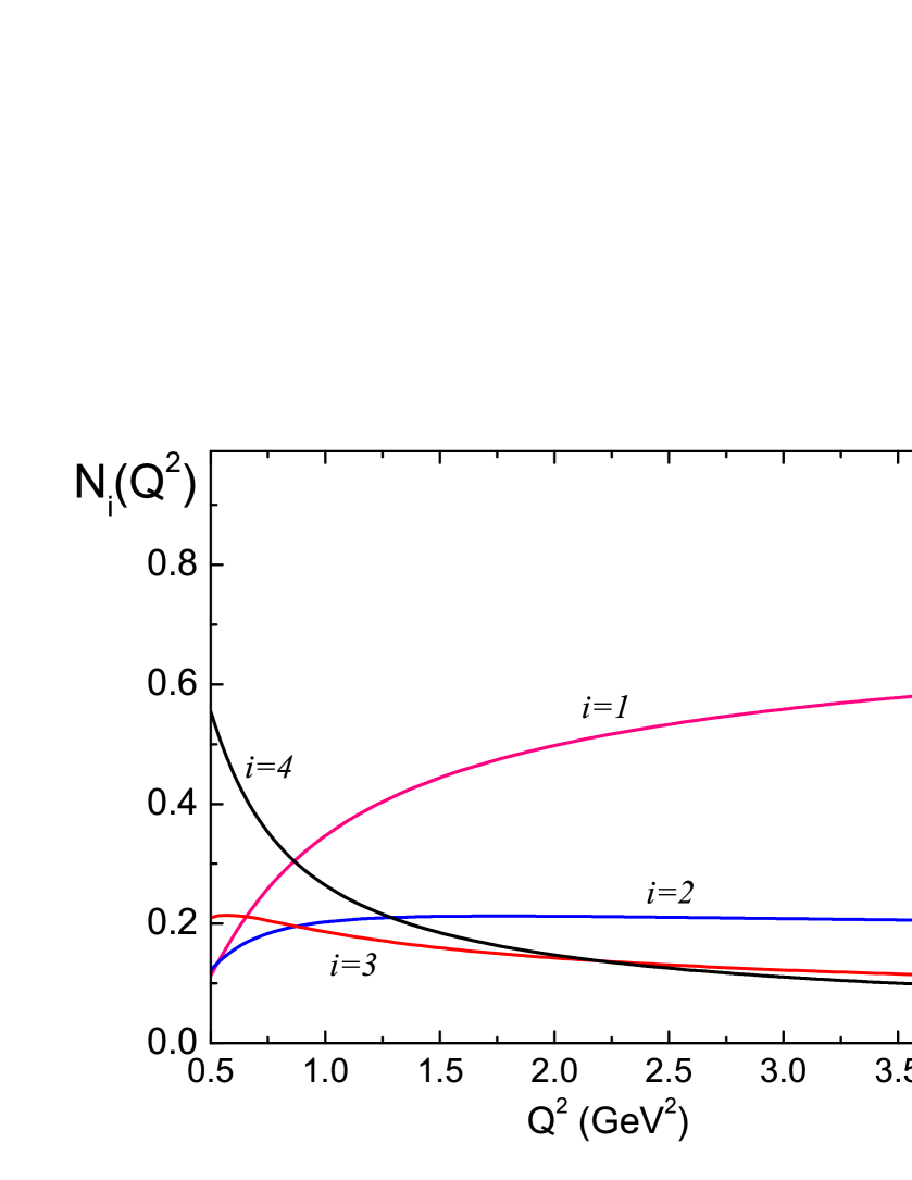
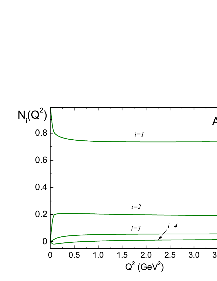
Figure 1: The $Q^{2}$-dependence of the relative contributions at the four-loop level in the PT approach.

      Figure 2: The $Q^{2}$-dependence of the relative contributions of the perturbative expansion terms in Eq. (19) in the APT approach.

As it is seen from Fig. 2, in the region $Q^{2}<1\,\text{GeV}^{2}$ the dominant contribution to the pQCD correction $\Delta_{\rm Bj}(Q^{2})$ comes from the four-loop term $\sim\alpha_{\rm s}^{4}$. Moreover, its relative contribution increases with decreasing $Q^{2}$. In the region $Q^{2}>2\,\text{GeV}^{2}$ the situation changes – the major contribution comes from one- and two-loop orders there. Analogous curves for the APT series given by Eq. (19) are presented in Fig. 2.

Figures 2 and 2 demonstrate the essential difference between the PT and APT cases, namely, the APT expansion obeys much better convergence than the PT one. In the APT case, the higher order contributions are stable at all $Q^{2}$ values, and the one-loop contribution gives about 70 %, two-loop – 20 %, three-loop – not exceeds 5%, and four-loop – up to 1 %.

One can see that the four-loop PT correction becomes equal to the three-loop one at $Q^{2}=2\,\text{GeV}^{2}$ and noticeably overestimates it (note that the slopes of these contributions are quite close in the relatively wide $Q^{2}$ region) for $Q^{2}\sim 1\,\text{GeV}^{2}$ which may be considered as an extra argument supporting an asymptotic character of the PT series in this region. In the APT case, the contribution of the higher loop corrections is not so large as in the PT one. The four-loop order in APT can be important, in principle, if the theoretical accuracy to better than 1 % will be required.

Now we briefly discuss how the APT applications affect the values of the higher-twist coefficients $\mu_{2i}^{p-n}$ in Eq. (17) extracted from Jlab data. Previously, a detailed higher-twist analysis of the four-loop expansions in powers of $\alpha_{\rm s}$ was performed in [39]. In Figs. 4 and 4 we present the results of 1- and 3-parametric fits in various orders of the PT and APT. The corresponding fit results for higher twist terms $\mu_{2i}^{p-n}$, extracted in different orders of the PT and APT, are given in Table 3 (all numerical results are normalized to the corresponding powers of the nucleon mass $M$).

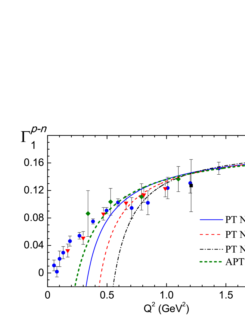
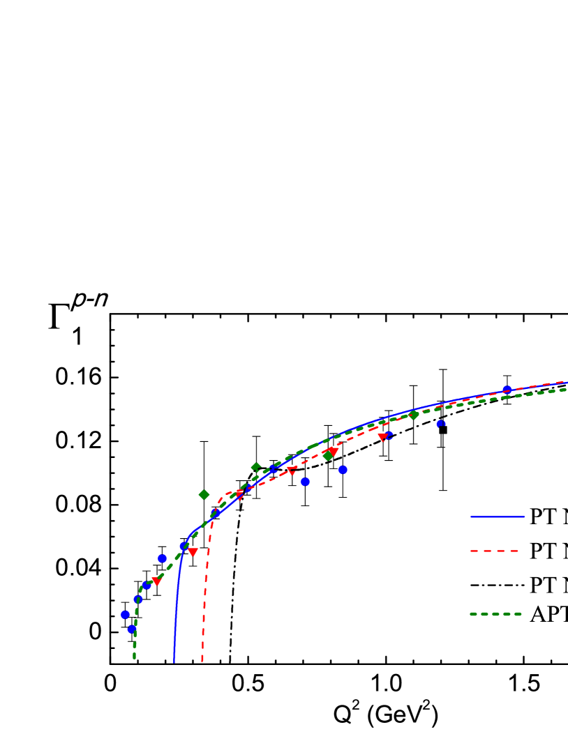
Figure 3: The one-parametric $\mu^{p-n}_{4}$-fits of the BSR JLab data in various (NLO, N²LO, N³LO) orders of the PT and the all-order APT expansions.

      Figure 4: The three-parametric $\mu^{p-n}_{4,6,8}$-fits of the BSR JLab data in various (NLO, N²LO, N³LO) orders of the PT and the all-order APT expansions.

Table 1: Results of higher twist extraction from the JLab data on BSR in various (NLO, N²LO, N³LO) orders of the PT and all orders of APT.

Method	$Q_{min}^{2},\,$	$\mu^{p-n}_{4}/M^{2}$	$\mu^{p-n}_{6}/M^{4}$	$\mu^{p-n}_{8}/M^{6}$
The best $\mu^{p-n}_{4}$-fit results
PT NLO	$0.5$	$-0.028(5)$	$-$	$-$
PT N2LO	$0.66$	$-0.014(7)$	$-$	$-$
PT N3LO	$0.71$	$~{}~{}0.006(9)$	$-$	$-$
APT	$~{}0.47$	$-0.050(4)$	$-$	$-$
The best $\mu^{p-n}_{4,6,8}$-fit results
PT NLO	$~{}0.27$	$-0.03(1)$	$-0.01(1)$	$0.008(4)$
PT N2LO	$0.34$	$~{}~{}0.01(2)$	$-0.06(4)$	$0.04(2)~{}$
PT N3LO	$0.47$	$~{}~{}0.05(4)$	$-0.2(1)~{}$	$0.12(6)~{}$
APT	$~{}0.08$	$-0.061(4)$	$0.009(1)$	$-0.0004(1)$

From these figures and Table 3 one can see that APT allows one to move down up to $Q^{2}\sim 0.1\,\text{GeV}^{2}$ in description of the experimental data [39]. At the same time, in the framework of the standard PT the lower border shifts up to higher $Q^{2}$ scales when increasing the order of the PT expansion. This is caused by extra unphysical singularities in the higher-loop strong coupling. It should be noted that the magnitude of $\mu^{p-n}_{4}/M^{2}$ decreases with an order of the PT and becomes compatible to zero at the four-loop level. It is interesting to mention that a similar decreasing effect has been found in the analysis of the experimental data for the neutrino-nucleon DIS structure function $xF_{3}$ [37] and for the charged lepton-nucleon DIS structure function $F_{2}$ [38].

Consider the application of the FAPT approach by the example of the RG-evolution of the non-singlet higher-twist $\mu^{p-n}_{4}(Q^{2})$ in Eq. (17). The evolution of the higher-twist terms $\mu^{p-n}_{6,8,\,...}$ is still unknown. The RG-evolution of $\mu^{p-n}_{4}(Q^{2})$ in the standard PT reads

$$\mu_{4,PT}^{p-n}(Q^{2}) = \mu_{4,PT}^{p-n}(Q_{0}^{2})\left[\frac{\alpha_{\rm s}(Q^{2})}{\alpha_{\rm s}(Q_{0}^{2})}\right]^{\nu}\,,\quad\nu=\gamma_{0}/\left(8\pi\beta_{0}\right)\,,\quad\gamma_{0}=\frac{16}{3}C_{F}\,,\quad C_{F}=\frac{4}{3}.$$ (20)

In the framework of FAPT the corresponding expression reads as follows:

$$\mu_{4,APT}^{p-n}(Q^{2})=\mu_{4,APT}^{p-n}(Q_{0}^{2})\,\frac{{\mathcal{A}}_{\nu}^{(1)}(Q^{2})}{{\mathcal{A}}_{\nu}^{(1)}(Q_{0}^{2})}.$$ (21)

We present in Table 2 the best fits for $\mu^{p-n}_{4}(Q_{0}^{2})$ taking into account the corresponding RG-evolution with $Q^{2}_{0}=1\,\text{GeV}^{2}$ as a normalization point and without the RG-evolution.

Table 2: Results of higher twist extraction from the JLab data on BSR with inclusion and without inclusion of the RG-evolution of $\mu_{4}^{p-n}(Q^{2})$ normalized at $Q^{2}_{0}=1\,\text{GeV}^{2}$.

$Method$	$Q_{min}^{2},\,\text{GeV}^{2}$	$\mu_{4}^{p-n}/M^{2}$	$\mu_{6}^{p-n}/M^{4}$	$\mu_{8}^{p-n}/M^{6}$
	0.47	$-0.055(3)$	0	0
NNLO APT	0.17	$-0.062(4)$	0.008(2)	0
no evolution	0.10	$-0.068(4)$	0.010(3)	$-0.0007(3)$
	0.47	$-0.051(3)$	0	0
NNLO APT	0.17	$-0.056(4)$	0.0087(4)	0
with evolution	0.10	$-0.058(4)$	0.0114(6)	$-0.0005(8)$

We do not take into account the RG-evolution in $\mu_{4}^{p-n}$ for the standard PT calculations and compare with FAPT since the only effect of that would be the enhancement of the Landau singularities by extra divergencies at $Q^{2}\sim\Lambda^{2}$, whereas at higher $Q^{2}\sim 1\,\text{GeV}^{2}$ the evolution is negligible with respect to other uncertainties. We see from Table 2 that the fit results become more stable with respect to $Q_{min}$ variations, which reduces the theoretical uncertainty of the BSR analysis.

4 Summary

To summarize, APT and FAPT are the closed theoretical schemes without unphysical singularities and additional phenomenological parameters which allow one to combine RG-invariance, $Q^{2}$-analyticity, compatibility with linear integral transformations and essentially incorporate nonperturbative structures. The APT provides a natural way for the coupling constant and related quantities. These properties of the coupling constant are the universal loop-independent infrared limit and weak dependence on the number of loops. At the same time, FAPT provides an effective tool to apply the Analytic approach for RG improved perturbative amplitudes. This approaches are used in many applications. In particular, in this paper we consider the application of APT and FAPT to the RG-evolution of nonsinglet structure functions and Bjorken sum rule higher-twist analysis at the scale $Q^{2}\sim\Lambda^{2}$ considered.

The singularity-free, finite couplings ${\cal A}_{\nu}(Q^{2}),{\mathfrak{A}}_{\nu}(s)$ appear in APT/FAPT as analytic images of the standard QCD coupling powers $\alpha_{\rm s}^{\nu}(Q^{2})$ in the Euclidean and Minkowski domains, respectively. In this paper, we presented the theoretical background, used in a package “FAPT” [29] based on the system Mathematica for QCD calculations in the framework of APT/FAPT, which are needed to compute these couplings up to N³LO of the RG running. We hope that this will expand the use of these approaches.

Acknowledgments

I am grateful to the organizers and conveniers of the ACAT2013 workshop for the invitation and for arranging such a nice even. In addition, I would like to thank Alexander Bakulev , Sergei Mikhailov and Andrei Kataev for stimulating discussions and useful remarks. This work was supported in part by the Belarussian state fundamental research programm “Convergency”, BelRFBR grants under Grant No. F12D-002 and No. F13M-143 and by RFBR Grant No. 11-01-00182.

References

References

- [1] Shirkov D V and Solovtsov I L 1997 Phys. Rev. Lett. 79 1209
- [2] Milton K A and Solovtsov I L 1997 Phys. Rev. D55 5295
- [3] Solovtsov I L and Shirkov D V 1999 Theor. Math. Phys. 120 1220
- [4] Shirkov D V 2001 Theor. Math. Phys. 127 409
- [5] Shirkov D V and Solovtsov I L 2007 Theor. Math. Phys. 150 132
- [6] Shirkov D V 2012 Nucl. Phys. Proc. Suppl. 225-227 5
- [7] Magradze B A 2000 Int. J. Mod. Phys. A15 2715
- [8] Kourashev D S and Magradze B A 2003 Theor. Math. Phys. 135 531
- [9] Magradze B A 2006 Few Body Syst. 40 71
- [10] Milton K A, Solovtsov I L, Solovtsova O P and Yasnov V I 2000 Eur. Phys. J. C14 495
- [11] Milton K A, Solovtsov I L and Solovtsova O P 2002 Phys. Rev. D65 076009
- [12] Cvetic G and Valenzuela C 2006 Phys. Rev. D74 114030
- [13] Cvetic G, Kogerler R and Valenzuela C 2010 J. Phys. G37 075001
- [14] Magradze B A 2010 Few Body Syst. 48 143
- [15] Milton K A, Solovtsov I L and Solovtsova O P 1998 Phys. Lett. B439 421
- [16] Pasechnik R S, Shirkov D V and Teryaev O V 2008 Phys. Rev. D78 071902
- [17] Milton K A, Solovtsov I L and Solovtsova O P 1999 Phys. Rev. D60 016001
- [18] Shirkov D V and Zayakin A V 2007 Phys. Atom. Nucl. 70 775
- [19] Baldicchi M, Nesterenko A V, Prosperi G M, Shirkov D V and Simolo C 2007 Phys. Rev. Lett. 99 242001
- [20] Bakulev A P, Mikhailov S V and Stefanis N G 2005 Phys. Rev. D72 074014, 2005 Erratum: ibid. D72 119908(E)
- [21] Bakulev A P, Mikhailov S V and Stefanis N G 2007 Phys. Rev. D75 056005, 2008 Erratum: ibid. D77 079901(E)
- [22] Bakulev A P 2009 Phys. Part. Nucl. 40 715
- [23] Broadhurst D J, Kataev A L and Maxwell C J 2001 Nucl. Phys. B592 247
- [24] Bakulev A P, Mikhailov S V and Stefanis N G 2010 JHEP 1006 085
- [25] Pasechnik R S, Shirkov D V, Teryaev O V, Solovtsova O P and Khandramai V L 2010 Phys. Rev. D81 016010
- [26] Cvetic G, Illarionov A Y, Kniehl B A and Kotikov A V 2009 Phys. Lett. B679 350
- [27] Kotikov A V, Krivokhizhin V G and Shaikhatdenov B G 2012 Phys. Atom. Nucl. 75 507
- [28] Ayala C and Cvetic G 2013 Phys. Rev. D87 054008
- [29] Bakulev A P and Khandramai V L 2013 Comput. Phys. Commun. 184 183
- [30] Nesterenko A V and Simolo C 2010 Comput. Phys. Commun. 181 1769
- [31] Nesterenko A V and Simolo C 2011 Comput. Phys. Commun. 182 2303
- [32] Chetyrkin K G, Kuhn J H and Steinhauser M 2000 Comput. Phys. Commun. 133 43
- [33] Beringer J et al. (Particle Data Group Collaboration) 2012 Phys. Rev. D86 010001
- [34] Gardi E, Grunberg G and Karliner M 1998 JHEP 07 007
- [35] Garkusha A V and Kataev A L 2011 Phys. Lett. B705 400
- [36] Baikov P A, Chetyrkin K G and Kühn J H 2010 Phys. Rev. Lett. 104 132004
- [37] Kataev A L, Parente G and Sidorov A V 2003 Phys. Part. Nucl. 34 20
- [38] Blumlein J 2013 Prog. Part. Nucl. Phys. 69 28
- [39] Khandramai V L, Pasechnik R S, Shirkov D V, Solovtsova O P and Teryaev O V 2012 Phys. Lett. B706 340