A Parametric Study Examining the Effects of Reshock in RMI

Abstract

The compression of a cylindrical gas bubble by an imploding molten lead (Pb) shell may be accompanied by the development of the Richtmyer-Meshkov (RM) instability at the liquid-gas interface due to the initial imperfection of the interface. A converging pressure wave impinging upon the interface causes a shell of liquid to detach and continue to travel inwards, compressing the gas bubble. The efficiency of compression and collapse evolution can be affected by development of the RM instability. Investigations have been performed in the regime of extreme Atwood number $A=-1$ with the additional complexity of modeling liquid cavitation in the working fluid. Simulations have been performed using the open source CFD software OpenFOAM on a set of parameters relevant to the prototype compression system under development at General Fusion Inc. for use as a Magnetized Target Fusion (MTF) driver.

After validating the numerical setup in planar geometry, simulations have been carried out in 2D cylindrical geometry for both initially smooth and perturbed interfaces. Where possible, results have been validated against existing theoretical models and good agreement has been found. While our main focus is on the effects of initial perturbation amplitude and azimuthal mode number, we also address differences between this problem and those usually considered, such as RM instability at an interface between two gases with a moderate density ratio. One important difference is the formation of narrow molten lead jets rapidly propagating inwards during the final stages of the collapse. Jet behaviour has been observed for a range of azimuthal mode numbers and perturbation amplitudes.

s

1 Introduction

When the interface between two fluids of different densities is subjected to rapid acceleration, e.g. by a shock passing through the interface, perturbations present at the interface prior to the passage of the wave grow with time. This phenomenon is known as the Richtmyer-Meshkov instability (RM) [1, 2], and has been extensively studied in the last couple of decades, mainly in the field of astrophysics. Recently, a renewed interest in RM was triggered by innovations in magnetized target fusion (MTF).

In this paper we study the cylindrical collapse of a gas cavity by an imploding liquid shell, where the development of interface instabilities is known to affect the compression efficiency. In this study we focus on the RM instability [1, 2], which is the first instability to develop on the liquid-gas interface during collapse. The MTF driver in development at General Fusion Inc. will compress a plasma-filled cylindrical cavity by using pneumatic pistons to initiate a converging pressure wave in molten lead (Pb). As the pressure wave reaches the liquid-plasma interface, the interface undergoes rapid acceleration and travels toward the center, compressing the plasma cavity. In our prototype device, the cavity is instead filled with argon gas. Perturbations existing at the liquid-gas interface prior to the passage of the pressure wave may seed the development of hydrodynamic instabilities. In this study, we concentrate on the parameter space relevant to our prototype device so as to define requirements for the smoothness of the initial liquid-gas interface for efficient compression.

The growth characteristics of initially small-amplitude sinusoidal perturbations can be divided into two regimes: (i) the linear regime, in which the contribution of nonlinear effects is negligible and evolution of the disturbance can be adequately described by the linearized equations, and (ii) the nonlinear regime, in which the perturbation growth decreases and finally saturates due to nonlinear effects. In the linear regime, initial perturbation growth can be reasonably predicted by the simple impulse models [1, 2] as $\dot{h}=h_{0}A\Delta U$, where $h_{0}$ is the initial perturbation amplitude, $\Delta U$ is the difference in the velocity of the interface before and after the passage of the shock wave, and $A$ is the Atwood number defined as $A=(\rho_{2}-\rho_{1})/(\rho_{2}+\rho_{1})$, where $\rho_{1}$ and $\rho_{2}$ are the fluid densities.

In literature, a characteristic pattern of RM instability is usually described in terms of fingers of one fluid penetrating into another. A finger of light fluid poking into heavy fluid is usually called a ‘bubble’, and that of heavy into light is called a ‘spike’. Bubbles and spikes grow at the same rate during the linear stage. However during the nonlinear stage, spikes undergo acceleration whereas bubbles tend to stagnate. The disparity in growth rates becomes more prominent at high Atwood numbers ($A\approx 1$), see e.g. Dimonte and Ramaprabhu [3], and in this regime a vast majority of the existing models also perform poorly.

Once the passing shock wave and the interface begin to interact, the evolution of the initially perturbed interface can be explained in terms of vorticity deposition. If the interface is perturbed, the pressure gradient of the shock is misaligned with the density gradient across the interface. This results in generation of the baroclinic vorticity through the term $\nabla\rho\times\nabla p$ in the vorticity equation. The sign of the generated vorticity (clockwise or counter clockwise) depends on the sign of the Atwood number, i.e. whether the shock travels from light fluid to heavy or vice versa [4, 5]. As such, the initial perturbation may grow monotonically or first decrease and then grow in the opposite direction, a phenomenon known as phase inversion [6, 5].

Most of the work to date on the RM instability has been carried out in rectangular geometry, with fluids modeled as ideal gases, and at moderate Atwood numbers ($|A|\approx 0.5-0.8$). A lot of effort was put into understanding the underlying physics, developing models describing nonlinear stages of disturbance evolution, and investigating the effects of compressibility, sensitivity to the initial conditions, and turbulent mixing, e.g. [7, 8, 4, 9, 3, 10, 11, 12]. Recently, there has been an increase in the number of works describing the RM instability in converging geometries [6, 13, 14, 15, 16, 17], which are more relevant to fusion. The situation in converging geometries is more complex than the planar case, because the trajectories of bubbles and spikes are no longer parallel as the interface moves in the radial direction. The evolution of small amplitude perturbations in cylindrical geometry was investigated by Mikaelian [16] for the case of pure azimuthal perturbations. Lombardini [17] extended the analysis [16] to also account for axial perturbations.

In converging geometries a fair bit of attention is devoted to the secondary effects, such as so-called ‘reshock’  [6, 14]; in planar geometry ‘reshock’ has been studied by [9]. When a shock wave strikes the interface between two fluids, it is partially transmitted into the second fluid and partially reflected. The transmission ratio depends on the acoustic impedance of each fluid, defined as $z=\rho c$, where $\rho$ and $c$ are the density and sound speed of the fluid, respectively. In a converging geometry the transmitted part of the shock travels to the origin, which acts as a singular point, and then bounces back to hit the interface again affecting the perturbation growth; this phenomenon is called ‘reshock’.

One of the aspects of the RM instability that has been given little attention until recently is the regime of high Atwood number ($A\approx\pm 1$). This situation occurs when a shock wave passes, for example, between a liquid and a gas. In this case, at least one of the fluids cannot be described as an ideal gas and other equations of state must be considered. If one of the fluids is a liquid and the shock reflects off the interface, cavitation can occur when the pressure falls below the tensile strength of the liquid, further increasing the complexity of the problem. A recent numerical study of Ward and Pullin [18] looks into the role that the equation of state has on RM instability growth in a planar geometry. An experimental study by Buttler et al. [19] investigates the RM instability at metal-vacuum interfaces in planar geometry. Their focus was on developing an ejecta source term model that links to the surface perturbations of shocked materials. The main assumption of their model is that ejecta formation at a metal-vacuum interface can be viewed as a special limiting case of the RM instability.

This numerical work focuses on the RM instability at a liquid-gas interface during a heavy-to-light implosion in cylindrical geometry. In this case, we have liquid $Pb$ surrounding a cylindrical cavity of air. The pressure pulse originates in the liquid and converges toward the liquid-gas interface. When the pressure pulse reaches the interface, it is almost entirely reflected because of the severe mismatch between the acoustic impedance of liquid $Pb$ and that of air. In this configuration, the reflected wave is a rarefaction wave that subjects the liquid to tension, which may cause cavitation.

The rest of this article is organized as follows. The problem statement and numerical method are described in $\S\ref{sec:method}$. The results of pulse propagation in liquid $Pb$ and collapse of the unperturbed cylindrical gas cavity are given in $\S\ref{sec:noPert}$. The effects of perturbation amplitude and azimuthal mode number on the RM instability growth rate are studied in $\S\ref{sec:RM}$. Finally, all results are summarized in $\S\ref{sec:Sum}$.

2 Problem Statement and Validation

2.1 Numerical Setup

Simulations are performed using the open source CFD code OpenFOAM [20]. A compressible multiphase solver ‘compressibleInterFoam’ is used for these simulations. This solver implements the Volume of Fluid (VoF) method for interface tracking and is suitable for the simulation of two compressible immiscible isothermal fluids. A barotropic equation of state is used to relate pressure and density for each phase:

$$\rho_{i}=\rho_{0_{i}}+\psi_{i}P,$$ (1)

where $\psi_{i}=1/c_{i}^{2}$ is the compressibility and $c_{i}$ is the speed of sound for phase $i$. For a gas (compressible) phase the nominal density $\rho_{0}$ in Eq. 1 is set to zero. This results in an ideal gas equation of state for an isothermal fluid. For a liquid (low compressibility phase) $\rho_{0}$ is set to the nominal density of the liquid under normal conditions. As such the fluid density remains essentially constant unless the liquid is subjected to very high pressures. Similar results can also be obtained using the Tait [21] equation of state for a liquid phase.

Simulations are carried out in 2D cylindrical geometry. A schematic of the numerical setup is shown in Fig. 1(a). The initial radius of the gas cavity and initial position of the interface is $R_{0}=0.2$ m. The outer boundary is at $R_{\mathrm{outer}}=1.5$ m, where a pressure pulse is imposed as a time-dependent pressure boundary condition $P(t)$. A typical pressure pulse is shown in Fig. 1(b). The maximum pressure and duration of the pulse are chosen to reflect the parameters of the prototype device, $P_{\mathrm{max}}=1.5$ GPa and $T_{\mathrm{pulse}}\approx 100$ $\mu$s in most simulations. A zero-gradient boundary condition is set for the velocity at the outer boundary allowing some mass influx into the domain. In most simulations a small central portion of the computational domain with radius $r<1$ cm has been excluded from the calculations to speed up the computations. The effect of excluding this central part was found to be negligible for the purposes of this work. The inner boundary uses an outflow boundary condition so that gas can ‘escape’ from the domain during the collapse. Both fluids are initially at rest at atmospheric pressure.

Simulations are carried out for both initially smooth and sinusoidally perturbed interfaces. The results for the unperturbed case are first validated against existing models and then used as a baseline of comparison for the growth of bubbles and spikes in perturbed interface runs.

The initial sinusoidal perturbation is defined by its initial amplitude $h_{0}$ and azimuthal mode wavenumber $n$, with a corresponding perturbation wavelength of $\lambda_{0}=2\pi R_{0}/n$.

The perturbation amplitude can be normalized relative to its wavelength, $h_{0}/\lambda_{0}$, as is done in planar geometry, or relative to the initial radius of the interface $h_{0}/R_{0}$.

Simulations with a coarse grid resolution in the radial direction ($\hat{r}$) are performed over the full azimuthal domain (Fig. 1a), while finer grid resolution runs are carried out over a restricted azimuthal angle $\theta_{\mathrm{segment}}$ (with periodic boundary conditions in the azimuthal direction) to speed up the calculations. The specific choice of $\theta_{\mathrm{segment}}$ depends on the azimuthal mode number $n$ of the perturbation used. The number of grid points in the radial direction is $N_{r}=2800$ and $N_{r}=11200$ for the coarse and fine resolution runs, respectively. The grid spacing is uniform for $r<R_{0}$ with $dr=2.375\times 10^{-4}$ m and $dr=5.9375\times 10^{-5}$ m for the coarse and fine grids, respectively. The smallest perturbation amplitude used in these simulations is $h_{0}=0.001$ m. This results in 17 fine grid points across the initial perturbation in the radial direction. The number of grid points per perturbation wavelength is set to $N_{\theta}=135$ in most simulations, although this is reduced to $N_{\theta}=55$ for high azimuthal mode perturbations.

Simulations are performed for an implosion of molten lead $Pb$ into air with the fluid properties $\rho_{Pb}=10000$ kg/m³, $c_{Pb}=2000$ m/s; $\rho_{\mathrm{air}}=1$ kg/m³, $c_{\mathrm{air}}=316$ m/s. The corresponding acoustic impedances are $z_{Pb}=2\times 10^{7}$ Rayl and $z_{\mathrm{air}}=316$ Rayl and the Atwood number is $A=(\rho_{\mathrm{air}}-\rho_{Pb})/(\rho_{\mathrm{air}}+\rho_{Pb})=-0.9998\approx-1$.

2.2 Validation Test

The numerical method and grid convergence are first tested in planar geometry on a set of parameters similar to those used in cylindrical geometry. The length of the computational domain in the streamwise direction ($\hat{x}$, normal to the interface) is $L_{x}=1.5$ m with the interface located at $X_{\mathrm{interface}}=1.3$ m. A pressure pulse $P(t)$ is prescribed at the inflow boundary at $X=0$ and an outflow (zero-gradient) boundary condition is used at $X=1.5$ m. The initial pressure pulse amplitude is $P_{max}=3.6$ GPa which roughly corresponds to the expected pressure at the interface in cylindrical geometry when the initial pulse amplitude is $P_{max}=1.5$ GPa (pressure is amplified due to the convergence). In the normal direction ($\hat{y}$, parallel to the surface of the interface) the length of the computational domain is one wavelength of a mode $n=6$ perturbation in the case of cylindrical geometry, $L_{y}=2\pi R_{0}/n=0.2094395102$ m. Periodic boundary conditions are imposed in the normal direction and the number of grid points set to be $N_{y}=135$, corresponding to the $n=6$ case in cylindrical geometry. Simulations are performed for three different grid resolutions in the streamwise direction. The grid spacing is uniform for $1.3$ m $\leq X\leq 1.5$ m and equal to $\Delta x=2.375\times 10^{-4}$, $1.1875\times 10^{-4}$ and $5.9375\times 10^{-5}$ m for grids with increasing resolution. The total number of grid points in the streamwise direction is correspondingly $N_{x}=2800$, $5600$ and $11200$.

A schematic of the flow pattern in the planar case is shown in Fig. 2. Part (a) of the figure shows propagation of the pressure pulse through $Pb$ prior to hitting the interface and part (b) illustrates the flow pattern some time after the pressure pulse hit the interface. The pressure pulse gets reflected from the interface as a rarefaction wave. This puts the liquid $Pb$ into tension and initiates cavitation behind the interface (Fig. 2b).

In planar geometry, an initially smooth interface is expected to move with constant velocity after interacting with the pressure pulse. In our case, the interface velocity $V_{\mathrm{interface}}$ can be approximated by assuming two fluids with a very large impedance ratio (see $\S 4.8$ and $\S 4.9$ in  [22]), such that,

$$V_{\mathrm{interface}}\approx 2V_{p}\,,$$ (2)

where $V_{p}$ is a particle velocity given by,

$$V_{p}=\frac{P_{\mathrm{max}}-P_{0}}{\rho_{Pb}c_{Pb}}\approx\frac{P_{\mathrm{max}}}{\rho_{Pb}c_{Pb}}.$$ (3)

The maximum pressure $P_{\mathrm{max}}$ and density $\rho_{Pb}$ of the pulse are taken just before it hits the interface. The ambient pressure is $P_{0}=1\times 10^{5}$ Pa.

The evolution of an initially smooth interface after it has been accelerated by a linearly ramped pressure pulse of infinite length is shown in Fig. 3 for two different grid resolutions. One can see that the grid resolution is sufficient to obtain well converged results. For our parameters, $P_{\mathrm{max}}\approx 3.6$ GPa, $\rho_{Pb}\approx 10500$ kg/m³ (there is a slight change in $Pb$ density as the pulse propagates through it due to compressibility) and $c_{Pb}\approx 2000$ m/s, the interface velocity predicted by Eq. 2 is $V_{\mathrm{interface}}=343$ m/s. The numerically calculated velocity (slope of the curve) is $U_{\mathrm{interface}}=344.7$ m/s, which deviates from the theoretical value by less than 0.5%.

An initially perturbed interface is also tested in planar geometry. The initial perturbation amplitude is set to $h_{0}=2$ mm (Fig. 2) and the perturbation wavelength $\lambda_{0}$ is equal to the length of the computational domain in the normal direction $\hat{y}$ leading to $h_{0}/\lambda_{0}=9.55\times 10^{-3}$.

In our analysis we follow the extrema points of the perturbations, marked by points $1$ and $2$ in Fig. 2, which we label, respectively, as bubbles and spikes throughout the entire simulation. It is important to note that during the first stage of the evolution phase inversion [6] occurs. This means that the perturbation which is initially a spike, i.e. heavy fluid surrounded by light fluid reverses to become a bubble; and vice-versa. As such our label ‘spike’ corresponds to a finger of a heavy fluid surrounded by light fluid once the phase inversion has occurred, whereas at early stages it is a finger of light fluid surrounded by heavy. The converse applies to bubbles.

Early evolution of the normalized spike amplitude is shown in Fig. 4 for pressure pulses of different duration, each with a maximum pressure of $P_{\mathrm{max}}=3.6$ GPa and modeled at the finest grid resolution. The spike amplitude has been calculated as the difference between the interface position at point $1$ for the case of a perturbed interface and the coincidental position of the initially unperturbed interface. One can see that for longer pulses ($T_{\mathrm{pulse}}\geq 200$ $\mu$s) the pulse length has no effect on the spike amplitude. However, if the pulse length falls below some threshold, the spikes’ amplitude growth slows down, clearly seen by comparing results in Fig. 4 for the shortest pulse $T_{\mathrm{pulse}}=100$ $\mu$s (red line) with those obtained for longer pulses.

Initial disturbance growth rates (indicated by the slope of the curves in Fig. 4) together with the growth rate predicted by the Richtmyer impulsive model [1] (given below by Eq. 4) for our set of parameters are listed in Table 2.

$$\dot{h}_{\mathrm{planar}}=h_{0}^{+}kA^{+}\Delta U,$$ (4)

where $k=2\pi/\lambda$ is the wave number of the perturbation, $h_{0}^{+}$ and $A^{+}$ are the initial post-shock amplitude and Atwood number, and $\Delta U$ is the velocity jump at the interface following passage of the shock. In our validation case we use $k=30$, $h_{0}^{+}=2$ mm, $A^{+}=1$, and $\Delta U=V_{\mathrm{interface}}=345$ m/s, resulting in $\dot{h}\approx 20.7$ m/s (see Table 2).

Our results for longer pulses agree well with the Richtmyer impulsive model, while for a shorter pulse the growth rate is lower.

3 Results

3.1 Pulse propagation and gas cavity collapse: unperturbed interface

In this section we study the collapse of an initially unperturbed gas cavity in 2D cylindrical geometry. The numerical results are validated against existing theoretical models and also used as a baseline for calculations of the perturbation growth for the runs with initially perturbed interfaces.

Propagation of a pressure pulse through the liquid $Pb$ from the outer boundary towards the interface in a cylindrical geometry is shown in Figure 5. The pressure pulse has a maximum initial amplitude of $P_{\mathrm{max}}=3.6$ GPa and duration $T_{\mathrm{pulse}}=100$ $\mu$s. It can be seen that the pressure pulse is amplified as it cylindrically converges in the $Pb$. This amplification is in excellent agreement with the theoretical prediction for a small amplitude (linear) pulse that is $P\sim 1/\sqrt{r}$ in cylindrical geometry [23]. (The pulse is expected to exhibit linear behaviour when the particle velocity is much less than the sound speed.) As the pulse approaches the interface and pressure becomes higher, nonlinearity starts to manifest itself by a steepening of the pulse front and a slight deviation of the amplitude from the theoretical curve. For the current set of parameters (near the interface: $P_{\mathrm{max}}\approx 3.6$ GPa, $\rho_{Pb}\approx 10500$ kg/m³ and $c_{Pb}\approx 2000$ m/s) the particle velocity of the pulse near the interface can be roughly estimated as $V_{p}\approx 171$ m/s by Eq. 3. This velocity is still relatively small (but not negligible) compared to the speed of sound ($171$ m/s compared to $2000$ m/s). Thus the pulse exhibits predominantly linear behaviour as it propagates through the $Pb$, although small nonlinear effects become noticeable near the interface. The time taken for the pulse to reach the interface $1.3$ m away is $t_{\mathrm{propagation}}=650$ $\mu$s, which agrees with the prescribed speed of sound $c_{Pb}=2000$ m/s. In subsequent results, time is defined relative to the moment the pressure pulse reaches the interface, such that $t=t_{\mathrm{sim}}-t_{\mathrm{propagation}}$.

A typical structure of the flow field during the collapse of an initially unperturbed cylindrical cavity is shown in Fig. 6 for a pressure pulse of duration $T_{\mathrm{pulse}}=100$ $\mu$s and maximum pressure $P_{\mathrm{max}}=1.5$ GPa. Parts (a) and (b) of the figure show volume of fluid (VoF) contours when the pressure pulse strikes the interface at $t=0$ and when the cavity has partially collapsed at $t=300$ $\mu$s, respectively. Part (c) shows the corresponding pressure contours at $t=300$ $\mu$s. It is worth reiterating that the imploding material is liquid $Pb$ with an acoustic impedance much larger than the air in the cavity. Therefore, the pressure pulse is almost completely reflected back into the $Pb$ as a rarefaction wave. The molten lead is then subjected to tension which causes it to cavitate. It is apparent in Fig. 6b that a $Pb$ shell is formed as a result of interaction between the pressure pulse and the liquid-gas interface. As the shell moves inwards, a cavitation region forms behind it, separating it from the rest of the molten lead. The pressure contours in Fig. 6c show that the $Pb$ shell becomes pressurized as it converges, while the pressure in the cavitation region falls to the minimum allowed by the numerical setup.

Radial profiles of the pressure, velocity and VoF at two different instances during the collapse ($t=100$ $\mu$s and $t=300$ $\mu$s) are shown in Fig. 7. We mainly focus on the behaviour of the molten lead as dynamics of the gas bubble has a very little effect on the liquid $Pb$ until the very late stages of the collapse. VoF profiles clearly show the location of the liquid-gas interface and growth of the cavitation region as the interface progresses inwards. Also evident is the increase in the thickness of the $Pb$ shell as it converges during the collapse process. From the pressure profiles we can see that the shell is pressurized as it moves toward the center. The pressure in the cavitation region becomes almost zero and the pressure inside the air increases as it is compressed. Velocity profiles indicate that the velocity gradually increases towards smaller radii both in the cavitation region and the $Pb$ shell, i.e. the inner edge of the shell is moving faster than its outer edge. During early stages of the collapse, the interface velocity (which is equal to the fluid velocity at the position of the interface) roughly corresponds to Eq. 2, but later increases due to the converging geometry.

If we look at the flow field structure inside the gas cavity one can observe a shock wave propagating through it. This shock wave is generated inside the air due to the sudden acceleration of the interface. The interface is analogous to a piston at rest that suddenly begins moving into a quiescent gas at constant velocity. In this situation, a shock front immediately appears, moving away from the piston with a constant supersonic speed. Ahead of the shock front the gas is at rest, while behind the shock it moves at the same velocity as the piston, i.e. the interface velocity in our case (see  [24] $\S 3$). Note that our numerical method is not sufficient for a high-accuracy solution of shock wave propagation inside the compressed gas. However, as mentioned earlier, the gas dynamics has little effect on the collapse therefore current numerical setup is sufficient for this study.

It is necessary to accurately predict the trajectory of the liquid-gas interface throughout the collapse so that the compression efficiency of our system can be estimated. The motion of an initially unperturbed interface in cylindrical geometry is shown in Fig. 8. The four different lines show our numerical results obtained for the pressure pulses of various durations and with maximum pressure $P_{\mathrm{max}}=1.5$ GPa. The theoretical solution of Kedrinskii ($\S$ 1.4 in  [25]) is also shown by the black solid line for comparison. One can see that the duration of the pulse influences the collapse time; longer pulses compress the cavity faster. This effect, however, diminishes as the pulse duration is increased, such that no difference in collapse time is observed for pulses with $T_{\mathrm{pulse}}\geq 400$ $\mu$s. Our results for the longer pulses are also in a very good agreement with a theoretical solution by Kedrinskii [25]) developed for studying underwater explosions. Some additional results concerning the effect of the pressure pulse amplitude as well as collapse characteristics of the initially unperturbed spherical cavity can be found in our earlier work [27].

It is worth noting that in the current numerical setup the gas never becomes sufficiently pressurized to affect the trajectory of the interface, which accelerates all the way to the axis due to geometrical convergence. In reality, however, the interface undergoes rapid deceleration during the very latest stages of compression because the gas pressure becomes comparable to the pressure in the $Pb$ shell. This deceleration is very important as the interface becomes Rayleigh-Taylor unstable during this phase.

3.2 The Richtmyer-Meshkov Instability

Now we turn our attention to the development of the RM instability during the collapse due to imperfections that may be present on the liquid-gas interface. In order to understand how various perturbations are going to affect the compression efficiency of our system, we study effects of the initial perturbation amplitude and azimuthal mode number. The parameters for each simulation are summarized in Table 2. In all cases, the pressure pulse has an amplitude of $P_{\mathrm{max}}=1.5$ GPa and a duration of $T_{\mathrm{pulse}}=100$ $\mu$s.

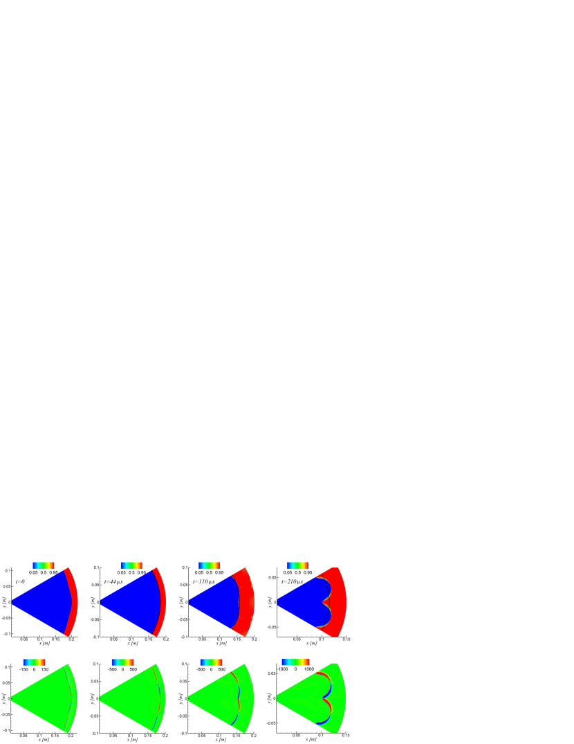
Figure 9: Early development of RM instability shown by VoF contours (first row) and contours of the vorticity component in $\hat{z}$ direction (units $[1/s]$) multiplied by VoF (second row). Initial perturbation is at azimuthal mode $n=12$ with amplitude of $h_{0}=2$ mm (Case N12A002 in Table 2). Black solid line shows interface position for initially unperturbed case. Pressure pulse has amplitude $P_{\mathrm{max}}=1.5$ GPa and duration $P_{\mathrm{pulse}}=100$ $\mu$s.

A typical perturbation evolution during the early and late stages of the collapse is shown in Figs. 9 and  10, respectively. In both figures, the VoF contours are plotted in the first row and the corresponding contours of the $\hat{z}$ vorticity component multiplied by VoF are plotted in the second row.

The position of the initially unperturbed interface is also shown by the black solid line. Results are presented for case N12A002 listed in Table 2 with an initial amplitude of $h_{0}=2$ mm and $n=12$.

One can see that once the pressure pulse interacts with the perturbed liquid-gas interface (Fig. 9 at $t=0$), vorticity is immediately generated in the vicinity of the interface because of initial misalignment of density and pressure gradients across the interface, i.e. the mechanism of baroclinic vorticity generation. For a pulse passing from a heavy fluid into a light one, the deposited vorticity initially acts in the direction opposite to that of the perturbation, smoothing the interface during the early evolution stages (Fig. 9 at $t=44$ $\mu$s). Vorticity then carries on to deflect the interface leading to the growth of the perturbation in the opposite direction, i.e. phase inversion (Fig. 9 at $t=110$ $\mu$s and $t=210$ $\mu$s). The asymmetry between the spikes and bubbles observed in Fig. 9 at $t=210$ $\mu$s indicates that the perturbation is entering a nonlinear stage of evolution.

There are two non-dimensional parameters that can be used to characterize evolution of the perturbation amplitude. The first one is the ratio of the perturbation amplitude and wavelength $h(t)/\lambda(t)$. Similar to the planar case, perturbation evolution is considered to be linear when $h(t)/\lambda(t)\ll 1$. However, in cylindrical geometry the wavelength of the perturbation decreases as the cavity is compressed so that nonlinear effects become prominent earlier. The second parameter is the ratio between the disturbance amplitude and radius of the cavity $h(t)/R(t)$. This parameter indicates how much the perturbation evolution is influenced by the curvature of the interface. For small amplitude initial disturbances parameter $h(t)/R(t)$ is small. At early stages of the collapse only low azimuthal modes are expected to be influenced by the curvature of the interface as they have significant ratios of $\lambda(t)/R(t)$, whereas early evolution of the perturbations at higher azimuthal modes is expected to be similar to that of the planar case. As the cavity continues to be compressed, however, the decrease in cavity radius increases the number of modes that are affected by curvature. Therefore, while the initial motion may be negligibly different from the planar case, we expect convergence effects to manifest themselves at some point during the collapse.

Keeping the above in mind we follow the spike evolution in Figs. 9 and 10. One can see that after phase inversion is complete ($t=110$, 210, and 312.5 $\mu$s), the spike amplitude grows, i.e. the distance increases between the crest of the perturbation and the position of the initially unperturbed interface. At later stages ($t=350$, 362.5, and 375 $\mu$s), the spike amplitude starts to decrease. This decrease in the perturbation amplitude correlates with the increase of parameter $h(t)/R(t)$. By examining the vorticity distribution, a reversal of the vorticity along the spike interface near the crest can be observed. This change in direction of rotation correlates with the direction of interface deflection, best seen by comparing times $t=210$ and 312.5 $\mu$s. One can also see the Kelvin-Helmholtz (K-H) instability that develops on the sides of the bubbles and spikes at later times $t>300$ $\mu$s, giving them a serrated appearance.

Another interesting phenomenon that can be observed in Figs. 9 and 10 is the formation of narrow molten lead jets (ribs) originating from the back of the bubble during the latest stages of the collapse ($t=350$, 362.5, and 375 $\mu$s). Formation of such jets has been observed in our simulations for perturbations with azimuthal mode numbers higher than four $(n>4)$. The prominence of the jets is dependent on the amplitude and mode of the initial perturbation. For this example case, the narrow jets only form but do not overtake the original spikes during the collapse. Instead, the spikes grew sufficiently to contact one another near the center, despite the deceleration they experience late in the collapse.

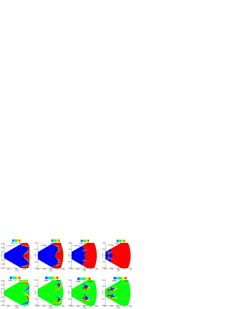
Figure 11: Formation of rib-like jets during late stages of collapse. VoF contours are shown in first row. Contours of vorticity component in $\hat{z}$ direction (units $[1/s]$) multiplied by VoF are shown in second row. Initial perturbation is mode $n=12$ with amplitude $h_{0}=1$ mm (Case N12A001 in Table 2). Black solid line shows interface position for initially unperturbed case. Pressure pulse has amplitude $P_{\mathrm{max}}=1.5$ GPa and duration $T_{\mathrm{pulse}}=100$ $\mu$s.

For the case of a perturbation with the same mode, but a lower initial amplitude, the situation is different, as shown in Fig. 11. This figure is in the same format as Fig. 10, but for case N12A001 in Table 2, which has a lower initial amplitude of $h_{0}=1$ mm. In this case these narrow molten lead jets move fast enough to overtake the original spikes and reach the center first. The results indicate that these narrow jets are also formed by redistribution of vorticity. We are not aware of such jets being observed in other works that use two gases with a moderate Atwood number as the working fluids. A very similar phenomenon has been observed, however, in the recent work of Enriquez et al. [28], in which an air cavity formed by collision of a solid body with a liquid reservoir collapses due to hydrostatic pressure (see Fig. 1 in [28]). The overall collapse process described in [28] is remarkably similar to the one obtained by our simulations.

3.2.1 Effect of Initial Perturbation Amplitude

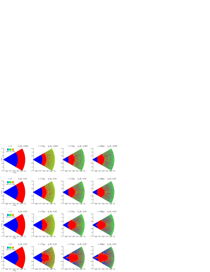
Figure 12: Effect of initial perturbation amplitude shown by VoF contours. Perturbation is mode $n=6$ and pressure pulse is $P_{\mathrm{max}}=1.5$ GPa. Each row of figure corresponds to a unique initial amplitude: $h_{0}=1$, 2, 4, and 10 mm; Cases N6A001, N6A002, N6A004, and N6A010 in Table 2.

The evolution of perturbations with various initial amplitudes is shown in Fig. 12 by VoF contours. Rows in the figure correspond to the evolution of $n=6$ perturbations with different initial amplitudes: cases N6A001, N6A002, N6A004 and N6A010 in Table 2. One can see that for the small amplitude initial perturbation (first row) no significant nonlinear effects are observed and the spikes and bubbles remain nearly symmetric throughout the time period shown. As the amplitude increases, nonlinear effects begin to manifest themselves in the growing asymmetry between the spikes and bubbles. The spike appears to accelerate and becomes sharper, whereas the bubble appears to stagnate. For the current Atwood number of $A\approx-1$, the spikes are significantly sharper than those simulated for lower Atwood numbers. This has also been observed by Tian et al. [14]. In addition, Fig. 12 illustrates that the shape of the molten lead shell surrounding the gas cavity is affected by the initial imperfections of the interface. The distortion of the shell increases as the initial perturbation amplitude is increased. For the largest tested amplitude (row four), the thickness of the shell behind the bubble almost goes to zero.

Before proceeding to the plots of the evolution of spikes and bubbles, we would like to once more clarify the notation being used in all our plots. We follow extrema of the perturbation throughout the entire simulation, therefore our notation of ‘spike’ and ‘bubble’ corresponds to that usually used in the literature from the moment the phase inversion has occurred, as explained earlier in the validation section.

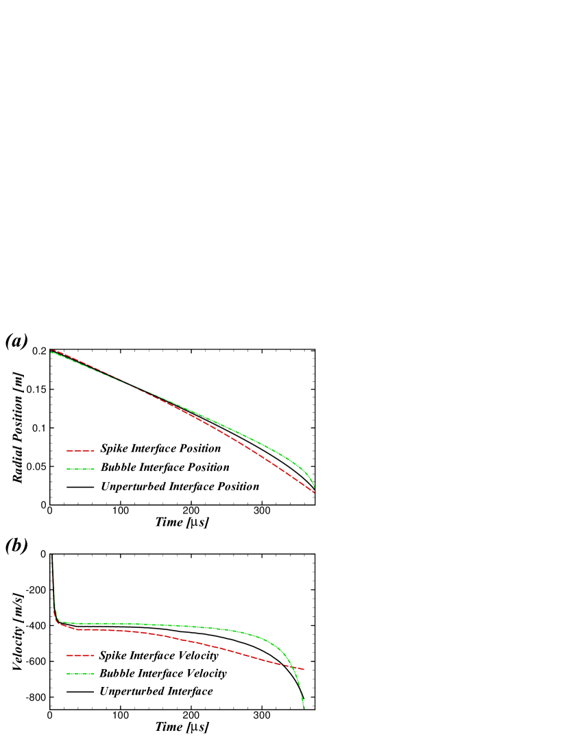
Figure 13: (a) Typical position of spike interface (red broken line), bubble interface (green dashed-dotted line), and initially unperturbed interface (black solid line); (b) Typical velocity of spike interface (red broken line), bubble interface (green dashed-dotted line), and initially unperturbed interface (black solid line). Case N6A002 in Table 2, pulse pressure $P_{\mathrm{max}}=1.5$ GPa, pulse length $T_{\mathrm{pulse}}=100$ $\mu$s.

This is illustrated in Fig. 13 for the case N6A002 in Table 2. Part (a) shows a typical evolution of the spike (red broken line) and bubble (green dash-dot line) interface position along with the position of the initially unperturbed interface (black solid line). Part (b) of the figure shows the corresponding interface velocities. Time $t=0$ corresponds to the moment when the pressure pulse hits the interface and the collapse begins. One can see that at $t=0$, the red and green lines corresponding to the maximum and minimum of the initial perturbation are above and below the radial position of the initially unperturbed interface (black line), respectively, and the difference between those lines defines the amplitude of the initial perturbation $h_{0}$. The perturbation decreases in amplitude until around $t\approx 100$ $\mu$s (when phase inversion occurs) and then starts to grow in the opposite direction. From that moment our notation of ’spike’ and ’bubble’ matches that commonly used in literature, i.e. a finger of light fluid poking into heavy fluid for a ‘bubble’, and that of heavy into light for a ‘spike’.

At late stages of the collapse the difference between red and black lines as well as between green and black lines starts to decrease again eventually accompanied by another reversal, which indicates formation of the narrow molten lead jets. Fig. 13 (b) shows the rapid acceleration of the interface resulting from its interaction with the pressure pulse. During early stages of the collapse, the velocities of the spikes, bubbles, and that of the unperturbed interface are nearly constant. Later the velocity of the unperturbed interface increases considerably due to the geometric convergence.

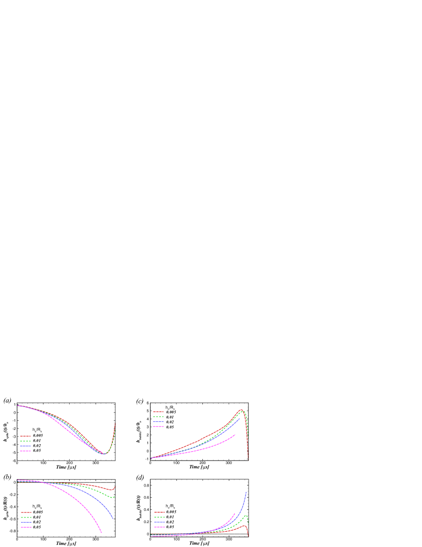
Figure 14: Effect of initial amplitude on perturbation growth. Left and right columns correspond to spike and bubble evolution. (a,c) Evolution of normalized perturbation amplitude; (b,d) Evolution of ratio between perturbation amplitude and radius of unperturbed gas cavity; Azimuthal mode number $n=6$, pressure pulse with $P_{max}=1.5$ GPa and $T_{pulse}=100$ $\mu$s.

The effect of initial amplitude on the perturbation growth is shown in Fig. 14 for cases N6A001, N6A002, N6A004 and N6A010 in Table 2. The left column (parts a and b) and the right column (parts c and d) in Fig. 14 show the amplitude evolution of the spikes and bubbles, respectively. The top row shows the amplitude normalized by its initial value $h_{0}$, while the bottom row shows the amplitude normalized by the radius of the unperturbed gas cavity $R(t)$.

Examining the growth characteristics of the spike we can observe the following: (i) at early times growth of the spikes scales well with the initial perturbation amplitude for all amplitudes under consideration, (ii) after the phase inversion when the curves cross zero for the first time, spike amplitude growth is faster for higher initial amplitudes, (iii) at large initial amplitudes the spike arrives at the center while it is still growing, so that no decrease of the spike amplitude is observed during the latest stages. For small initial amplitudes the spikes experience deceleration during late times, leading to a rapid decrease in spike amplitude. By comparing the growth characteristics of spikes and bubbles, it is apparent that the bubble amplitude does not scale as well with the initial perturbation amplitude, even early in the collapse. The bubble amplitude growth is significantly reduced for larger initial perturbations when compared to smaller ones. For the small amplitude perturbations, a decrease in bubble amplitude can be seen at the latest stages. This decrease is related to formation of the rib-like jets and their rapid propagation toward the center of the cavity, as discussed earlier.

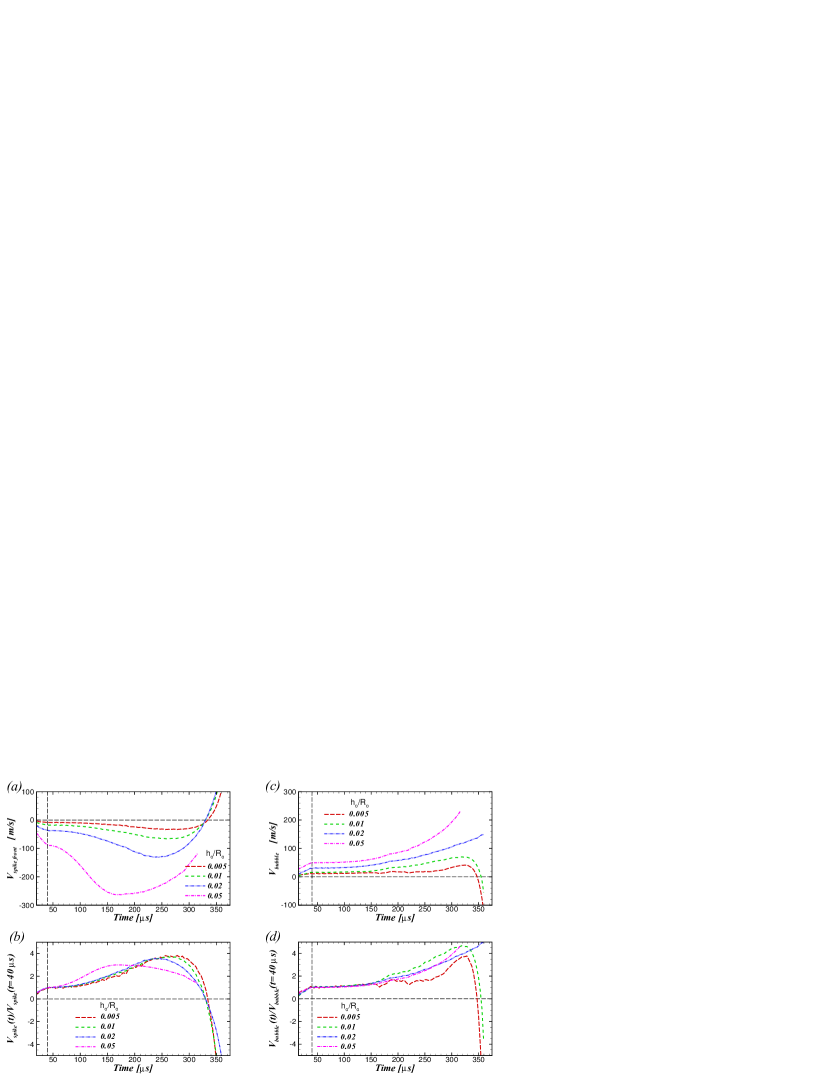
Figure 15: Effect of initial amplitude on perturbation growth rate. Left and right columns correspond to spike and bubble evolution, respectively. (a,c) Perturbation growth rate; (b,d) Perturbation growth rate normalized by its initial growth rate at $t=40$ $\mu$s. Azimuthal mode number $n=6$, pulse pressure $P_{\mathrm{max}}=1.5$ GPa, pulse length $T_{\mathrm{pulse}}=100$ $\mu$s.

The effect of initial amplitude on the growth rates of spikes and bubbles is shown in Fig. 15. The left and right columns of the figure show the velocities of the spikes and bubbles (relative to the velocity of the unperturbed interface) corresponding to the data in Fig. 14. Dimensional velocities are plotted in the first row of the figure and the same velocities normalized by the corresponding velocity at $t=40$ $\mu$s (immediately after the initial acceleration of the interface has been completed) are plotted in the second row. In Figs. 14(a) and 14(c) a negative velocity corresponds to the situation in which the perturbed interface (either spike or bubble) moves inwards faster than the initially unperturbed interface, whereas a positive velocity indicates that the perturbed interface moves inwards slower than the unperturbed interface (although it still moves inwards).

From the velocity plots one can see that after some finite initial time required to accelerate the interface from rest ($t\approx 40$ $\mu$s), the velocities of both spikes and bubbles approach a nearly constant value for a little while. This value is taken as the initial velocity that is used for scaling. Both spikes and bubbles undergo gradual acceleration until late times, when there is rapid deceleration, except for cases with large initial amplitudes in which the spikes reach the axis before this decelerate phase can occur. For all amplitudes under consideration, the bubble growth rate scales well with initial bubble velocity until the collapse is well underway. The spike growth rate also scales well, except for large amplitude perturbations, in which the growth rate saturates more quickly than the other cases.

3.2.2 Effect of Azimuthal Mode Number

The behaviour of spikes and bubbles is tested for various representative azimuthal mode numbers in the range $3\leq n\leq 32$, with the results displayed in Fig. 16. The left columns (parts a, b, and c) and the right columns (parts d, e, and f) correspond to the evolution of spikes and bubbles, respectively. The first row of the figure (parts a and d) shows amplitude evolution of spikes and bubbles normalized by the initial perturbation amplitude $h_{0}$. The second row (parts b and e) shows a zoomed-in section of the first row plot together with the theoretical model for the small amplitude perturbations of Mikaelian [16] (green dashed lines). Finally, the third row (parts c and f) show the same data when time is scaled by the mode $n$. All simulations have been carried out for an initial perturbation amplitude of $h_{0}/R_{0}=0.005$.

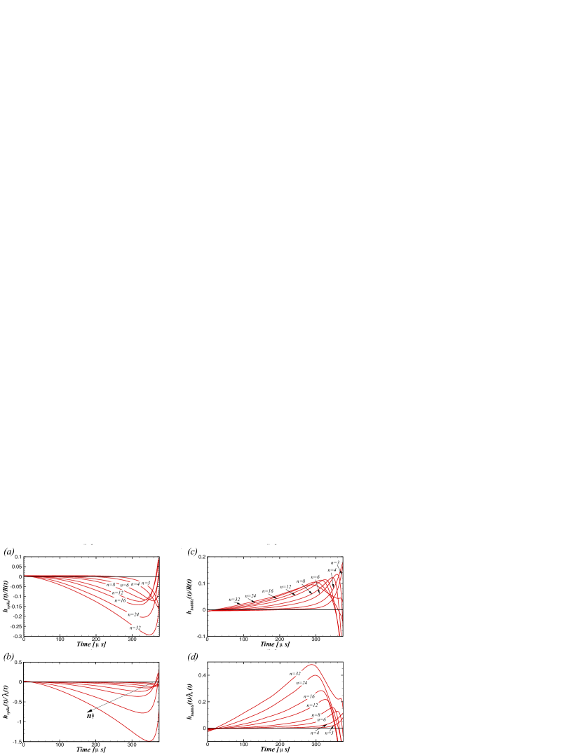
Figure 17: Effect of azimuthal mode number $n$ on perturbation evolution. Left and right columns correspond to the spike and bubble evolution, respectively. (a,c) Evolution of ratio between perturbation amplitude and radius of unperturbed gas cavity; (b,d) Evolution of the ratio between perturbation amplitude and wavelength. Pressure pulse with $P_{\mathrm{max}}=1.5$ GPa and $T_{\mathrm{pulse}}=100$ $\mu$s.

From the plots shown in Fig. 16 the following can be observed: (i) for the setup and parameters under consideration the perturbation evolution at low azimuthal numbers ($n=3,4$) differs from that at higher azimuthal mode numbers. In particular, the decrease in the perturbation amplitude (and in most cases a second phase inversion) observed at higher azimuthal modes at the latest stages of the collapse does not occur at low azimuthal mode numbers; (ii) at higher azimuthal modes ($n=24,32$) the maximum amplitude attained by spikes is significantly higher than that of bubbles; (iii) the initial evolution of spikes agrees well with Mikaelian’s theoretical model [16] for perturbations with large $n$. The predictions of the theoretical model are less favorable for bubble evolution; (iv) the phase inversion time roughly scales with the azimuthal mode number; (v) the second phase inversion, due to formation of the narrow (rib-like) jets at the head of each bubble, is clearly seen in parts (c) and (f) of the figure. However, in the case of large azimuthal mode, the cavity collapses before the second phase inversion is completed, as can be seen from the $n=32$ curves. Fig. 17 shows the same results as in Fig. 16, but with the perturbation amplitude normalized by the cavity radius $R(t)$ (first row) and perturbation wave length $\lambda(t)$ (second row). The left and right columns of the figure correspond to the spike and bubble evolution, respectively. One can see that at later stages of the collapse, both ratios, $h(t)/R(t)$ and $h(t)/\lambda(t)$ attain significant values for all perturbations being considered. This implies that both the nonlinear effects and the effect of the interface curvature become important for all perturbations at some point during the collapse.

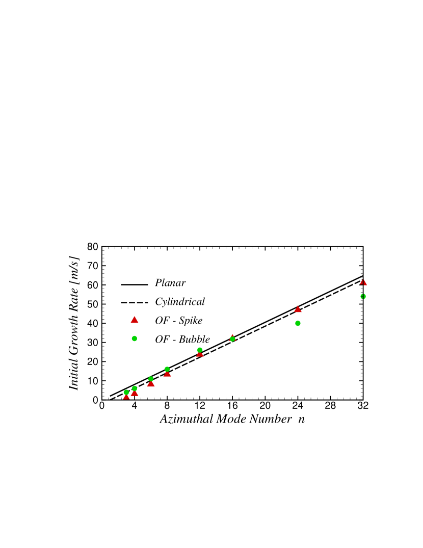
Figure 18: Effect of azimuthal mode number on perturbation early growth rate. Red triangles and green circles correspond to initial growth rates of spikes and bubbles, respectively. Solid line is planar model of Richtmyer [1] (Eq. 6). Dashed line is cylindrical model of Mikaelian [16] (Eq. 7). Pressure pulse with $P_{\mathrm{max}}=1.5$ GPa and $T_{\mathrm{pulse}}=100$ $\mu$s.

Finally, Fig. 18 shows the effect of the azimuthal mode number on the initial perturbation growth rate, taken at $t\approx 40$ $\mu$s, after the initial acceleration of the interface has been completed. The growth rates of spikes and bubbles are shown by red triangles and green circles, respectively. Here we reiterate that these initial growth rates are calculated before any of the azimuthal modes have completed phase inversion. Therefore, the ‘spikes’ and ‘bubbles’ referred to in the legend of Fig. 18 are outward and inward bulges, respectively.

The data is fitted to two linear models. The first is that of Richtmyer [1] for planar geometry,

$$\dot{h}_{\mathrm{planar}}=h_{0}kAV_{\mathrm{interface}},$$ (6)

where as usual, $h_{0}$ denotes the initial perturbation amplitude, $A$ is an Atwood number, $k=2\pi/\lambda=n/R_{0}$ is the wave number, $n$ is the azimuthal mode, and $V_{\mathrm{interface}}$ is the initial velocity of the undisturbed interface (see Eq. 2). The second model is that of Mikaelian [16] for cylindrical geometry,

$$\dot{h}_{\mathrm{cylindrical}}=(nA-1)\frac{h_{0}}{R_{0}}V_{\mathrm{interface}},$$ (7)

where $R_{o}$ is the initial radial position of the interface. The growth rate given by the planar model is shown by the solid line, while that of the cylindrical model is shown by the dashed line.

The growth rates presented in Fig. 18 show encouraging agreement with linear models for the range of perturbations being considered. It can be also seen that there is a change in the growth rates pattern for the higher azimuthal modes ($n>16$ based of the our data set). This is probably because of more pronounced nonlinear effects at those modes: in all our simulations the parameter $h_{o}/R_{o}$ has been kept constant and therefore, the parameter $h_{o}/\lambda_{o}$ increases with the increase in the azimuthal mode number of the perturbation. One can also see some mismatch in the initial growth rates of spikes and bubbles at lower azimuthal modes. This disparity becomes less pronounced as azimuthal mode of the perturbation increases (up to $n=16$).

4 Summary

In this work, the behaviour of the Richtmyer-Meshkov instability was studied for the case of a cylindrical gas (air) bubble compressed by an imploding molten lead shell. The main contribution of this work is to explore the RM instability in the extreme regime of Atwood number $A=-1$ with a liquid (molten lead) as one of a working fluids. Our motivation is to estimate the minimum smoothness required to achieve efficient compression of the gas cavity. Simulations have been performed using OpenFOAM software for a set of parameters relevant to the prototype compression system under development at General Fusion Inc. as a driver for magnetized target fusion. The main results and conclusions are summarized below:

• In the regime of Atwood number $A=-1$, there is a disparity between the growth rates of spikes and bubbles; spikes undergo acceleration while bubbles move at nearly constant velocity. This disparity in growth rates becomes more prominent as the amplitude of the initial perturbation is increased.

• The shape of the spikes obtained for the current set of parameters is different from that usually observed in the regime of moderate Atwood numbers. The spikes retain a sharp point with the Kelvin-Helmholtz instability producing serrated sides; they do not develop into the typical mushroom shape.

• During the latest stages of the collapse, when the non-dimensional parameters $\lambda(t)/R(t)$ and $h(t)/R(t)$ are no longer small, the spike amplitude starts to decrease. For some range of perturbation azimuthal modes and amplitudes, this is the onset of a second phase inversion.

• The formation of narrow molten lead jets propagating inwards and originating from the top of the bubbles has been observed during the latest stages of the collapse for modes $n>4$. To the best of our knowledge these jets have not been observed at a gas-gas interface with moderate Atwood number.

• To maintain sufficient compression efficiency, low-mode interface perturbations are not likely to be detrimental. However, high-mode perturbations are problematic and must be kept to a minimum.

This numerical setup seems to produce valuable results despite its lack of sophisticated modeling for all physical phenomena involved. It will be interesting to explore the effect of incorporating more physics into the simulation. There is also opportunity to further examine the effects of cavitation model, shock wave capturing scheme, rotation of the fluid and magnetic field on the dynamics of the gas cavity collapse.

Table 1: Planar Case: Initial Growth Rate

Case	$h_{0}[m]$	$T_{\mathrm{pulse}}\,[\mu s]$	$\dot{h}\,[m/s]$
Richtmyer model [1] (Eq. 4)	$0.002$	infinite	$20.7$
OpenFOAM simulation	$0.002$	infinite	$23.0$
OpenFOAM simulation	$0.002$	$100$	$9.8$

Table 2: List of parameters for the simulations performed

No.	Name	n	$h_{0}$ [m]	$h_{0}/R_{0}$	$h_{0}/\lambda_{0}$
1	N3A001	3	0.001	0.005	0.002387
2	N4A001	4	0.001	0.005	0.003183
3	N6A001	6	0.001	0.005	0.004775
4	N8A001	8	0.001	0.005	0.006366
5	N12A001	12	0.001	0.005	0.009549
6	N12A002	12	0.002	0.010	0.019098
7	N16A001	16	0.001	0.005	0.01273
8	N24A001	24	0.001	0.005	0.01909
9	N32A001	32	0.001	0.005	0.02546
10	N6A002	6	0.002	0.010	0.009549
11	N6A004	6	0.004	0.020	0.01909
12	N6A010	6	0.010	0.050	0.04775
13	N3A004	3	0.004	0.020	0.009549
14	N3A008	3	0.008	0.040	0.01909

Figure 1: (a) Numerical setup for 2D simulations in a cylindrical geometry; (b) Typical shape of the pressure pulse imposed on the outer boundary.

Figure 2: Schematic of a test case in planar geometry. (a) Pressure pulse propages through $Pb$ prior to hitting the $Pb$-air interface. (b) Some time after the pressure pulse hits the $Pb$-air interface.

Figure 3: Planar geometry: Evolution of the initially smooth interface for two grid resolutions. Pressure pulse is of an infinite length and amplitude $P_{\mathrm{max}}=3.6$ GPa.

Figure 4: Planar geometry: Early evolution of the normalized spike amplitude for pressure pulses with various lengths. Maximum pulse pressure is $P_{\mathrm{max}}=3.6$ GPa and initial perturbation amplitude is $h_{0}/\lambda=9.55\times 10^{-3}$ .

Figure 5: Pressure pulse propagation from the outer boundary at $r=1.5$ m towards the interface at $r=0.2$ m in cylindrical geometry. Initial pulse amplitude is $P_{\mathrm{max}}=1.5$ GPa and pulse duration is $T_{\mathrm{pulse}}=100$ $\mu$s. The pulse propagates from left to right.

Figure 6: Typical structure of the flow field during compression of initially unperturbed gas cavity by pressure pulse with $T_{\mathrm{pulse}}=100$ $\mu$s and $P_{\mathrm{max}}=1.5$ GPa. (a) Volume of fluid (VoF) contours when the pressure pulse hits the interface; (b) Volume of fluid (VoF) and (c) pressure contours when the cavity has partially collapsed at $t=300$ $\mu$s.

Figure 7: Typical structure of the flow field during compression of initially unperturbed gas cavity by pressure pulse with $T_{\mathrm{pulse}}=100$ $\mu$s and $P_{\mathrm{max}}=1.5$ GPa. Radial profiles of VoF (blue dash-dot line), pressure (green solid line), and velocity (red broken line) during the collapse. (a) $t=100$ $\mu$s and (b) $t=300$ $\mu$s.

Figure 8: Effect of pressure pulse duration $T_{\mathrm{pulse}}$ on motion of liquid-gas interface during collapse of initially unperturbed cylindrical cavity. Semi-analytical solution of Kedrinski [25] is also plotted as black solid line. Maximum pulse pressure is $P_{\mathrm{max}}=1.5$ GPa.

Figure 10: Late development of RM instability shown by VoF contours (first row) and contours of vorticity component in $\hat{z}$ direction (units $[1/s]$) multiplied by VoF (second row). Initial perturbation is at azimuthal mode $n=12$ with amplitude of $h_{0}=2$ mm (Case N12A002 in Table 2). Black solid line shows interface position for initially unperturbed case. Pressure pulse has amplitude $P_{\mathrm{max}}=1.5$ GPa and duration $P_{\mathrm{pulse}}=100$ $\mu$s.

Figure 16: Effect of the azimuthal mode number $n$ on perturbation growth. Left and right columns correspond to spike and bubble evolution, respectively. (a,d) Normalized perturbation amplitude; (b,e) zoom of (a,d) (red solid lines) along with small amplitude theoretical model of Mikaelian [16] (green broken lines); (c,f) time scaled by mode $n$. Pressure pulse with $P_{\mathrm{max}}=1.5$ GPa and $T_{\mathrm{pulse}}=100$ $\mu$s.

References

- [1] R. D. Richtmyer, Taylor instability in shock acceleration of compressible fluids, Commun. Pure Appl. Math. 13 (1960) 297–319.
- [2] E. E. Meshkov, Instability of the interface of two gases accelerated by a shock wave, Fluid Dyn. 4(5) (1969) 101–104.
- [3] G. Dimonte, P. Ramaprabhu, Simulations and model of the nonlinear Richtmyer-Meshkov instability, Phys. Fluids 22 (2010) 014104.
- [4] M. Brouillette, The Richtmyer-Meshkov instability, Annu. Rev. Fluid Mech. 34 (2002) 445–468.
- [5] N. J. Zabusky, Vortex paradigm for accelerated inhomogeneous flows: Visiometrics for the Rayleigh-Taylor and Richtmyer-Meshkov environments, Annu. Rev. Fluid Mech. 31 (1999) 495–536.
- [6] Q. Zhang, M. J. Graham, A numerical study of Richtmyer-Meshkov instability driven by cylindrical shocks, Phys. Fluids 10 (1998) 974–992.
- [7] Y. Yang, Q. Zhang, D. H. Sharp, Small amplitude theory of Richtmyer-Meshkov instability, Phys. Fluids 6 (1994) 1856–1873.
- [8] R. L. Holmes, G. Dimonte, B. Fryxell, M. L. Gittings, J. W. Grove, M. Schneider, D. H. Sharp, A. L. Velikovich, R. P. Weaver, Q. Zhang, Richtmyer-Meshkov instability growth: experiment, simulation and theory, J. Fluid Mech. 389 (1999) 55–79.
- [9] M. Latini, O. Schilling, W. S. Don, High-resolution simulations and modeling of reshocked single-mode Richtmyer-Meshkov instability: Comparison to experimental data and to amplitude growth model predictions, Phys. Fluids 19 (2007) 024104.
- [10] K. Nishihara, J. G. Wouchuk, C. Matsuoka, R. Ishizaki, V. V. Zhakhovsky, Richtmyer-Meshkov instability: theory of linear and nonlinear evolution, Phil. Trans. R. Soc. A 368 (2010) 1769–1807.
- [11] B. Thornber, D. Drikakis, D. L. Youngs, R. J. R. Williams, The influence of initial conditions on turbulent mixing due to Richtmyer-Meshkov instability, J. Fluid Mech. 654 (2010) 99–139.
- [12] R. H. Cohen, W. P. Dannevik, A. M. Dimits, D. E. Eliason, A. A. Mirin, Y. Zhou, Three-dimensional simulation of a Richtmyer-Meshkov instability with a two-scale initial perturbation, Phys. Fluids 14 (2002) 3692–3709.
- [13] J. R. Fincke, N. E. Lanier, S. H. Batha, R. M. Hueckstaedt, G. R. Magelssen, S. D. Rothman, K. W. Parker, C. J. Horsfield, Postponement of saturation of the Richtmyer-Meshkov instability in a convergent geometry, Phys. Rev. Letters 93(11) (2004) 115003.
- [14] B. Tian, D. Fu, Y. Ma, Numerical investigation of Richtmyer-Meshkov instability driven by cylindrical shocks, Acta Mech Sinica 22 (2006) 9–16.
- [15] R. Krechetnikov, Rayleigh-Taylor and Richtmyer-Meshkov instabilities of flat and curved interfaces, J. Fluid Mech. (2009) 625–387.
- [16] K. O. Mikaelian, Rayleigh-Taylor and Richtmyer-Meshkov instabilities and mixing in stratified cylindrical shells, Phys. Fluids 17 (2005) 094105.
- [17] M. Lombardini, D. I. Pullin, Small-amplitude perturbations in the three-dimensional cylindrical Richtmyer-Meshkov instability, Phys. Fluids 21 (2009) 114103.
- [18] G. M. Ward, D. I. Pullin, A study of planar Richtmyer-Meshkov instability in fluids with Mie-Gruneisen equations of state, Phys. Fluids 23 (2011) 076101.
- [19] W. T. Buttler, D. M. Oro, D. L. Preston, K. O. Mikaelian, F. J. Cherne, R. S. Hixson, F. G. Mariam, C. Morris, J. B. Stone, G. Terrones, D. Tupa, Unstable Richtmyer-Meshkov growth of solid and liquid metals in vacuum, J. Fluid Mech. 703 (2012) 60–84.
- [20] OpenFOAM, Manual, www.openfoam.org.
- [21] P. G. Tait, Report on some of the physical properties of fresh water and sea water, Rept. Sci. Results Voy., H.M.S. Challenger, Phys. Chem. 2 (1888) 1–76.
- [22] P. A. Thompson, Compressible Fluid Dynamics, Maple Press Company, 1984.
- [23] L. D. Landau, E. M. Lifshitz, Fluid Mechanics, 2nd Edition, Pergamon Press, 1987.
- [24] R. Courant, K. O. Friedrichs, Supersonic Flow and Shock Waves, Springer-Verlag, 1976.
- [25] V. K. Kedrinskii, Hydrodynamics of Explosion, Springer-Verlag, 2005.
- [26] R. H. Cole, Underwater Explosions, Dover, New York, 1965.
- [27] V. Suponitsky, S. Barsky, A. Froese, On the collapse of a gas cavity by an imploding molten lead shell and Richtmyer-Meshkov instability, In Proceedings of the 20th Annual conference of the CFD Society of Canada, Canmore, Alberta, Canada, May 9-11, 2012.
- [28] O. R. Enriquez, I. R. Peters, S. Gekle, L. E. Schmidt, M. Versluis, et al., Collapse of nonaxisymmetric cavities, Phys. Fluids 22 (2010) 091104.