A High Order Time Splitting Method Based on Integral Deferred Correction for Semi-Lagrangian Vlasov Simulations

Andrew Christlieb , Wei Guo , Maureen Morton , Jing-Mei Qiu

Abstract. Semi-Lagrangian schemes with various splitting methods, and with different reconstruction/interpolation strategies have been applied to kinetic simulations. For example, the order of spatial accuracy of the algorithms proposed in [Qiu and Christlieb, J. Comp. Phys., 2010] is very high (as high as ninth order). However, the temporal error is dominated by the operator splitting error, which is second order for Strang splitting. It is therefore important to overcome such low order splitting error, in order to have numerical algorithms that achieve higher orders of accuracy in both space and time. In this paper, we propose to use the integral deferred correction (IDC) method to reduce the splitting error. Specifically, the temporal order accuracy is increased by $r$ with each correction loop in the IDC framework, where $r=1,\,2$ for coupling the first order splitting and the Strang splitting, respectively. The proposed algorithm is applied to the Vlasov-Poisson system, the guiding center model, and two dimensional incompressible flow simulations in the vorticity stream-function formulation. We show numerically that the IDC procedure can automatically increase the order of accuracy in time. We also investigate numerical stability of the proposed algorithm via performing Fourier analysis to a linear model problem.

Keywords: Vlasov-Poisson system; Guiding center model; Operator/dimensional splitting; Semi-Lagrangian method; WENO reconstruction; Integral deferred correction.

1 Introduction

In this paper, we propose a semi-Lagrangian (SL) algorithm for Vlasov simulations, that is designed to be high order accurate in both space and time. In the proposed scheme, we utilize the high order weighted essentially non-oscillatory (WENO) spatial reconstructions [29, 30, 31], coupled to a dimensional splitting SL framework, originally proposed in [6], with an integral deferred correction (IDC) framework [14, 12].

A simple collisionless model in describing plasma is given by the Vlasov-Poisson (VP) system,

$$f_{t}+{\bf v}\cdot\nabla_{\bf x}f+{\bf E}(t,{\bf x})\cdot\nabla_{\bf v}f =0,$$ (1.1)

$${\bf E}(t,{\bf x})=-\nabla_{\bf x}\phi,\quad-\Delta_{\bf x}\phi =-1+\rho(t,{\bf x}),$$ (1.2)

where $f(t,{\bf x},{\bf v})$ describes the probability of finding a particle with velocity ${\bf v}\in\mathcal{R}^{3}$ at position ${\bf x}\in\mathcal{R}^{3}$ at time $t$, ${\bf E}$ is the electrostatic field, $\phi$ is the self-consistent electrostatic potential, and $\rho(t,{\bf x})=\int{f(t,{\bf x},{\bf v})d{\bf v}}$ is the electron charge density and the $1$ represents the uniformly distributed infinitely massive ions in the background. All physical constants in (1.1) have been normalized to one.

Popular numerical approaches in solving the VP system can be classified as three types: Eulerian, Lagrangian and SL. The Lagrangian type particle methods, e.g. particle-in-cell (PIC) [3, 23, 40], evolve the solution by following the trajectories of some sampled macro-particles, while the Eulerian approach [43, 8, 7] evolves the state variable according to the PDE on a fixed numerical grid. The SL approach is a mixed approach of Lagrangian and Eulerian in the sense that it has a fixed numerical grid; however, over each time step the state variable is evolved by propagating information along characteristics. The Eulerian and the SL approaches can be designed to be of very high order accuracy, an advantage when compared with the Lagrangian approach. On the other hand, because of the evolution mechanism, the SL method does not suffer the CFL time step restriction as in the explicit Eulerian approach, allowing for extra large time step evolution, and therefore less computational effort.

The SL approach is very popular in numerical weather prediction [36, 18] and kinetic simulations [1, 2, 24, 15, 39], among many others. In kinetic simulations of plasma, a very popular approach is the Strang splitting SL method, first proposed by Cheng and Knorr [6]. The advantage of performing such a splitting is that the decoupled lower dimensional equations of spatial advection and velocity ac/decelaration respectively are linear and are much easier to evolve numerically. Because of this, numerical schemes with high order of spatial accuracy have been designed, and demonstrated numerically to be more efficient than lower order schemes in finite difference framework with different reconstruction/interpolation strategies, such as, the cubic spline interpolation [35], the cubic interpolated propagation [27], the WENO interpolation [5, 29, 30]; in finite volume framework for the VP system [16] and for the guiding center Vlasov equation [13]; and in finite element discontinuous Galerkin framework [33, 32]. On the other hand, the numerical error in time is dominated by the splitting error, which is relatively low order ($\mathcal{O}(\Delta t^{2})$). In this paper, we will adopt the idea of integral deferred correction (IDC) to correct lower order dimensional splitting error.

The IDC methods are considered one-step, multi-stage integrators for solving initial value problems (IVPs). They are motivated by the defect/deferred correction (DC) methods [37, 17, 28], and more recently the spectral deferred correction (SDC) methods [14]. By construction, the IDC framework can systematically extend simple low order time integrators to high order ones by correcting provisional solutions. The DC/SDC/IDC methods and their variants have been applied to many application areas such as chemical rate equations, reactive flow [25, 4], hyperbolic equations [41], and parabolic equations [9]. Additionally, recent developments in IDC algorithms have opened up new possibilities for increased computational speed via parallelization [10].

In this paper, we investigate applying the IDC framework to correct the dimensional splitting error in solving the VP system, and guiding center models with plasma applications, as well as in simulating incompressible flows. We choose the dimensional splitting SL finite difference WENO scheme [29, 30] as the base solver in the prediction and correction steps of IDC, but point out that SL finite difference schemes with different reconstruction procedures such as those in [35, 26, 5] can also be used. In the IDC framework, the low order temporal accuracy from dimensional splitting is increased by iteratively approximating error functions via solving error equations. In particular, the temporal error accuracy is lifted by $r$ in each correction loop, where $r=1,\,2$ for coupling the first order splitting and the Strang splitting, respectively. Our proposed SL scheme coupled with the IDC method enjoys the simplicity of the dimensional splitting algorithm, maintains the high order spatial accuracy, and can be designed to be of high order in time. However, the IDC methods with correction steps will render some CFL time step restrictions. We perform linear stability analysis via the classic Fourier approach and provide upper bounds of the CFL numbers for the proposed schemes. The CFL time step restriction is comparable to that for Eulerian methods using Runge-Kutta time discretization, leading to the computational cost at a similar scale.

We would like to remark that prior to the proposed IDC method in correcting the dimensional splitting error, several constructions of high order splitting methods have been developed. The methods proposed in [42, 20] are in the spirit of composition methods, requiring backward steppings (negative time steps). The number of intermediate stages, hence the computational cost, increases exponentially with the order of the splitting method. A fourth order splitting in [42] is applied to the VP system in [33]. Higher order splitting methods that do not require backward steppings by using complex coefficients are proposed in [21]. The number of intermediate stages scales similarly to [42]. A fourth order splitting method for a linear Vlasov equation was presented in [34]. However, the generalization of this fourth order method to a nonlinear problem is not straightforward.

The paper is organized as follows. Section 2 is a review of the dimensional splitting SL WENO method for the VP system. Section 3 first reviews the IDC method for IVPs in Section 3.1, then formulates the error equations for the dimensional splitting algorithm for the VP system in Section 3.2. The algorithm is then extended to guiding center models in Section 3.3. Section 4 investigates the numerical stability via symbolic Fourier analysis for a linear model problem. Section 5 demonstrates the performance of the proposed schemes in simulating the VP system, the guiding center model, and advection in incompressible flow. Finally, a conclusion is given in Section 6.

2 Dimensional splitting SL WENO method for the VP system

This section is a brief review of the dimensional splitting SL WENO algorithm for solving the VP system [29, 30]. The proposed algorithm is up to ninth order accurate in phase space, but subject to dimensional splitting error. The main procedures are outlined below. For simplicity, we consider the problem with only 1-D in space and 1-D in velocity. The domain $(x,v)\in[0,L]\times[-v_{max},v_{max}]$. The boundary condition is periodic in the $x$-direction, and zero boundary condition is assumed in the $v$-direction.

Dimensional splitting. The time splitting form of equation (1.1) is,

$$f_{t}+v\cdot f_{x}=0~{},~{}$$ (2.1)

$$f_{t}+E(t,{x})\cdot f_{v}=0~{}.~{}$$ (2.2)

The splitting form of equation (1.1) is first order accurate if one evolves equation (2.1) for a full time step, then solving the Poisson’s equation (1.2) for electrostatic field $E({x})$ and finally evolves equation (2.2) for another full time step in a sequential way. It can be designed to be second order accurate in time by solving equation (2.1) for a half time step, the solving the Poisson’s equation for $E({x})$, then solving equation (2.2) for a full time step, followed by solving equation (2.1) for a second half time step, i.e., Strang splitting [38].

SL WENO scheme. The splitting strategy decouples the nonlinearity of the Vlasov equation into two linear hyperbolic equations (2.1) and (2.2). The linearity of 1-D equations allows for a simple implementation of high order SL methods. For example, the conservative SL finite difference WENO schemes proposed for 1-D equations such as equation (2.1) or (2.2) have been shown to be successful due to the conservative nature of the scheme formulation, the flexibility of working with point values, the stability and robustness of WENO reconstruction and the large time step efficiency of SL methods [30]. We briefly review the methodology below and refer readers to [30] for more details.

We adopt the following notations for the numerical discretization. The phase space is discretized by the following uniformly distributed grid points

$$0=x_{0}<\cdots<x_{i}\cdots<x_{N_{x}}=L,$$

$$-v_{max}=v_{0}<\cdots<v_{j}<\cdots<v_{N_{v}}=v_{max},$$

where $x_{i}=i\cdot\Delta x$ with mesh size $\Delta x=L/N_{x}$ and $v_{j}=-v_{max}+j\cdot\Delta v$ with mesh size $\Delta v=2v_{max}/N_{v}$. Let $x_{i+1/2}=(x_{i}+x_{i+1})/2$, $v_{j+1/2}=(v_{j}+v_{j+1})/2$. Let $f^{n}_{ij}$ be the point value of numerical solution at $x=x_{i}$, $v=v_{j}$ and $t=n\Delta t:=t_{n}$.

Take equation (2.1) for example: the SL finite difference WENO scheme is based on integrating the conservative form of equation (2.1) for some fixed $v_{j}$, over $[t_{n},t_{n+1}]$,

$$f(t_{n+1},x,v_{j})=f(t_{n},x,v_{j})-\left(\int_{t_{n}}^{t_{n+1}}v_{j}f(\tau,x,v_{j})d\tau\right)_{x}.$$

For simplicity of notation, we omit the $v_{j}$-dependence below under the dimensional splitting framework. Let $f^{n}_{i}\doteq f(t^{n},x_{i},v_{j})$. Evaluating the above equation at the grid point $x_{i}$ gives

$$f^{n+1}_{i} =f^{n}_{i}-\left.\left(\int_{t_{n}}^{t_{n+1}}vf(\tau,x)d\tau\right)_{x}\right|_{x=x_{i}}=f^{n}_{i}-\mathcal{F}_{x}\Big{|}_{x=x_{i}},$$ (2.3)

where $\mathcal{F}(x)\doteq\int_{t_{n}}^{t_{n+1}}vf(\tau,x)d\tau$. Let $\mathcal{H}(x)$ be a function whose sliding average is $\mathcal{F}(x)$, i.e.,

$$\mathcal{F}(x)=\frac{1}{\Delta x}\int_{x-\frac{\Delta x}{2}}^{x+\frac{\Delta x}{2}}\mathcal{H}(\xi)d\xi.$$ (2.4)

Taking the $x$ derivative of the above equation gives

$$\mathcal{F}_{x}=\frac{1}{\Delta x}\left(\mathcal{H}(x+\frac{\Delta x}{2})-\mathcal{H}(x-\frac{\Delta x}{2})\right).$$

Therefore the equation (2.3) can be written in a conservative form as

$$f^{n+1}_{i}=f^{n}_{i}-\frac{1}{\Delta x}(\mathcal{H}(x_{i+\frac{1}{2}})-\mathcal{H}(x_{i-\frac{1}{2}})),$$ (2.5)

where $\mathcal{H}(x_{i+\frac{1}{2}})$ is called the flux function. By following information along characteristics, $\mathcal{F}(x_{i})=\int_{t_{n}}^{t_{n+1}}vf(\tau,x_{i})d\tau=\int_{x_{i}^{\star}}^{x_{i}}fd\xi$ can be evaluated by reconstructing function $f$ at $t_{n}$ from neighboring point values. We denote this reconstruction procedure as $\mathcal{R}_{1}$. Similar to the idea in the finite difference WENO scheme, $\mathcal{H}(x_{i+\frac{1}{2}})$ can be reconstructed in high order from several of its neighboring cell averages

$$\bar{\mathcal{H}}_{k}=\frac{1}{\Delta x}\int_{x_{k-\frac{1}{2}}}^{x_{k+\frac{1}{2}}}\mathcal{H}(\xi)d\xi\stackrel{{\scriptstyle\eqref{eq: H}}}{{=}}\mathcal{F}(x_{k}),\quad k=i-p,\cdots,i+q.$$

We denote this reconstruction procedure as $\mathcal{R}_{2}$. In summary, a SL finite difference scheme in evolving equation (2.1) from $t_{n}$ to $t_{n+1}$ can be designed as follows:

1. At each of the grid points at time level $t_{n+1}$, say $(x_{i},t_{n+1})$, trace the characteristic back to time level $t_{n}$ at $x^{\star}_{i}=x_{i}-v\Delta t$.

2. Reconstruct $\mathcal{F}(x_{i})=\int_{t_{n}}^{t_{n+1}}vf(\tau,x_{i})d\tau=\int_{x_{i}^{\star}}^{x_{i}}fd\xi$ from $\{f^{n}_{i}\}_{i=1}^{N_{x}}$. We use $\mathcal{R}_{1}$ to denote this reconstruction procedure $\mathcal{R}_{1}[x_{i}^{\star},x_{i}](f^{n}_{i-p_{1}},\cdots,f^{n}_{i+q_{1}})$ in approximating $\mathcal{F}(x_{i})$, where $(i-p_{1},\cdots,i+q_{1})$ indicates the stencil used in the reconstruction. $\mathcal{R}_{1}[a,b]$ indicates the reconstruction of $\int_{a}^{b}f(t,\xi)d\xi$.

3. Reconstruct $\{\mathcal{H}(x_{i+\frac{1}{2}})\}_{i=0}^{N_{x}}$ from $\{\bar{\mathcal{H}}_{i}\}_{i=1}^{N_{x}}$. We use $\mathcal{R}_{2}$ to denote this reconstruction procedure $\hat{F}_{i+\frac{1}{2}}\doteq\mathcal{R}_{2}(\bar{\mathcal{H}}_{i-p_{2}},\cdots,\bar{\mathcal{H}}_{i+q_{2}})$ in approximating $\mathcal{H}(x_{i+\frac{1}{2}})$, where $(i-p_{2},\cdots,i+q_{2})$ indicates the stencil used in the reconstruction.

4. Update the solution $\{f^{n+1}_{i}\}_{i=1}^{N_{x}}$ by

   $$f^{n+1}_{i}=f^{n}_{i}-\frac{1}{\Delta x}(\hat{F}_{i+\frac{1}{2}}-\hat{F}_{i-\frac{1}{2}}),$$ (2.6)

   with numerical fluxes $\hat{F}_{i\pm\frac{1}{2}}$ computed in the previous step.

When the reconstruction stencils in $\mathcal{R}_{1}$ and $\mathcal{R}_{2}$ above only involve one neighboring point value of the solution, then the scheme is first order accurate in space. In fact, the scheme reduces to a first order upwind scheme when the time step is within CFL restriction. The proposed SL finite difference scheme can be designed to be of high order accuracy by including more points in the stencil for $\mathcal{R}_{2}\circ\mathcal{R}_{1}$, the composition of $\mathcal{R}_{1}$ and $\mathcal{R}_{2}$, to reconstruct the numerical flux

$$\hat{F}_{i+\frac{1}{2}}=\mathcal{R}_{2}\circ\mathcal{R}_{1}(f^{n}_{i-p},\cdots,f^{n}_{i+q}),$$ (2.7)

where $(i-p,\cdots,i+q)$ indicates the stencil used in the reconstruction process. The WENO mechanism can be introduced in reconstruction procedures as a stable and non-oscillatory method to capture fine scale structures. The details of the design of high order SL WENO algorithm are described in [30]. It is numerically demonstrated in [29, 30, 31] that the proposed high order SL WENO method works very well in Vlasov simulations with extra large time step evolution.

The computational procedure for the first order dimensional splitting SL finite difference WENO scheme for the VP system is summarized by the flow chart below.

Algorithm 1: A first order dimensional splitting SL finite difference WENO scheme for the VP system: 1. Evolve the solution $f^{n}$ by solving equation (2.1) to advect in $x$-direction for a time step $\Delta t$ with a SL finite difference WENO scheme (2.6), where the numerical flux $\hat{F}_{i+\frac{1}{2}}$ is reconstructed by (2.7) in a WENO fashion. Denote the solution after the evolution by $f^{n,*}$. 2. Solve electrostatic field $E^{n,*}$ induced by $f^{n,*}$ from the Poisson’s equation using a fast Fourier transform (FFT). 3. Evolve the solution $f^{n,*}$ by solving equation (2.2) to advect in $v$-direction for a time step $\Delta t$ to get $f^{n+1}$ as step 1.

Remark 2.1.

Algorithm 1 can be improved into second order in time by adopting Strang splitting as we mentioned at the beginning of Section 2.

Remark 2.2.

There are different conservative SL finite difference procedures proposed in [29, 30, 31]. These approaches have similar performance for linear advection equations with constant coefficients. However, we choose to review the SL procedure from [30], as it is more general in the sense that it can be applied to linear advection equations with variable coefficients. For solving the VP system, the methodologies proposed in [29, 30, 31] can be applied. However, for the guiding center model in Section 3.3, the dimensional splitting equations have variable coefficients. Hence, the above reviewed procedure from [30] is needed.

3 IDC methods for improving the temporal order of accuracy

In this section, we first briefly review the IDC procedure for initial value problems [14, 12]. Then we introduce the proposed IDC scheme in reducing the dimensional splitting error for the VP system in Section 3.2 and for the guiding center model in Section  3.3.

3.1 Overview of IDC methods

We provide a brief review of IDC methods [12], designed for scalar/system of initial value problems in the following form,

$$\left\{\begin{array}[]{l}\displaystyle y^{\prime}(t)=g(t,y),\quad t\in[0,T],\\ \displaystyle y(0)=y_{0}.\end{array}\right.$$ (3.1)

The time domain, $[0,T]$, is discretized into intervals,

$$0=t_{1}<t_{2}<\cdots<t_{n}<\cdots<t_{N}=T,$$

and each interval, $I_{n}=[t_{n},t_{n+1}]$, is further discretized into sub-intervals,

$$t_{n}=t_{n,0}<t_{n,1}<\cdots<t_{n,m}<\cdots<t_{n,M}=t_{n+1}.$$ (3.2)

The IDC method on each time interval $[t_{n},t_{n+1}]$ is described below. We drop the subscript $n$, e.g., $\tau_{0}:=t_{n,0}$ in (3.2), with the understanding that the IDC method is described for one time interval. We also refer to $\tau_{m}:=t_{n,m}$ as grid points or quadrature nodes, whose index $m$ runs from $0$ to $M$. In the IDC method, the size of sub-intervals are uniform. Let $\Delta\tau\doteq\frac{t_{n+1}-t_{n}}{M}$, then $\tau_{m}=t_{n}+m\Delta\tau$, $m=0,\ldots,M$. The procedure of an IDC method with $M+1$ uniformly distributed quadrature nodes as in equation (3.2) and with $K$ correction loops denoted as IDC$(M+1)$J$(K)$ is the following:

1. (prediction step) Use a low order numerical method to obtain a numerical solution, $\vec{\eta}^{[0]}=(\eta^{[0]}_{0},\ldots,\eta^{[0]}_{m},\ldots,\eta^{[0]}_{M}),$ which is a low order approximation to the exact solution at quadrature points. For example, applying a first order forward Euler method to (3.1) gives

   $$\eta^{[0]}_{m+1}=\eta^{[0]}_{m}+\Delta\tau g(t,\eta^{[0]}_{m}),\,m=0,\ldots,M-1.$$

2. (correction loops) Use the error function to improve the accuracy of the scheme at each iteration.
   For $k=1,\ldots,K$ ($K$ is the number of correction steps)

   1. Denote the error function from the previous step as

      $$e^{(k-1)}(t)=y(t)-\eta^{(k-1)}(t),$$

      where $y(t)$ is the exact solution and $\eta^{(k-1)}(t)$ is an $M^{th}$ degree polynomial interpolating $\vec{\eta}^{[k-1]}$.

   2. Denote the residual function as

      $$\epsilon^{(k-1)}(t)=(\eta^{(k-1)})^{\prime}(t)-g(t,\eta^{(k-1)}(t)).$$

   3. Compute the numerical error vector, $\vec{\delta}^{[k]}=(\delta^{[k]}_{0},\ldots,\delta^{[k]}_{m},\ldots,\delta^{[k]}_{M})$, using a low order numerical method to discretize the following error equation with a zero initial condition,

      $$\left(e^{(k-1)}+\int_{0}^{t}\!\!\epsilon^{(k-1)}(\tau)\,d\tau\right)^{\prime}\!\!(t) =g(t,\eta^{(k-1)}(t)+e^{(k-1)}(t))-g(t,\eta^{(k-1)}(t)).$$ (3.3)

      For example, applying a first order forward Euler scheme to equation (3.3) gives

      $$\delta^{[k]}_{m+1}=\delta^{[k]}_{m}+\Delta\tau(g(\tau_{m},\eta^{[k-1]}_{m}+\delta^{[k]}_{m})-g(\tau_{m},\eta_{m}^{[k-1]}))+\sum_{\ell=0}^{M}{\alpha_{m,\ell}~{}g(\tau_{\ell},\eta_{\ell}^{[k-1]})}$$

      $$+\eta_{m}^{[k-1]}-\eta_{m+1}^{[k-1]},\quad m=0,\ldots,M-1.$$ (3.4)

      To get equation (2c) from the discretization of (3.3), $\int_{\tau_{m}}^{\tau_{m+1}}\epsilon^{(k-1)}(t)\,dt$ is approximated by

      $$\eta_{m+1}^{[k-1]}-\eta_{m}^{[k-1]}-\sum_{\ell=0}^{M}{\alpha_{m,\ell}~{}g(\tau_{\ell},\eta_{\ell}^{[k-1]})},$$

      where $\sum_{j=0}^{M}{\alpha_{m,\ell}~{}g(\tau_{\ell},\eta_{\ell}^{[k-1]})}$ approximates $\int_{\tau_{m}}^{\tau_{m+1}}g(t,\eta^{(k-1)}(t))dt$ by quadrature formulas. We note that such a way of evolving the error function in the IDC algorithm is advantageous compared with that in the traditional DC algorithm. It introduces more stability by using the integral form, rather than the differentiation form, of the residual.

   4. Update the numerical solution $\vec{\eta}^{[k]}=\vec{\eta}^{[k-1]}+\vec{\delta}^{[k]}$.

Remark 3.1.

(About notations.) In our description of IDC, we let English letters $y_{m}$, $e^{(k)}_{m}$ denote the exact solutions and exact error functions, and Greek letters ${\eta}^{[k]}_{m}$, ${\delta}^{[k]}_{m}$ denote the numerical approximations to the exact solutions and error functions. We use subscript $m$ to denote the location $t=\tau_{m}$. The superscripts $k$ with round brackets ($(k)$) and square brackets ($[k]$) are for functions and vectors (or their components) respectively at the prediction ($k=0$) and correction loops ($k=1,\ldots,K$). We let $\vec{\cdot}$ denote the vector on IDC quadrature nodes. For example, $\vec{y}=(y_{0},\ldots,y_{M})$.

Remark 3.2.

(About the distribution of the quadrature nodes.) The IDC methods reviewed above adopt the uniformly distributed quadrature nodes to compute the residual. In [12], it is proved under some mild assumption, that the order accuracy of a IDC method can be increased by $r$ order when an $r^{th}$ order Runge-Kutta integrator is used to solve the error equation in each correction loop. The numerical results reported in [11] show that such high order accuracy lifting property does not always hold for an SDC method, which is constructed with Gaussian quadrature nodes.

Remark 3.3.

(About computational cost and storage requirement.) In terms of the order of accuracy, per $\Delta\tau$ (a subinterval size in the IDC method), numerical solutions $\eta^{[K]}_{m}$ are $(K+1)^{th}$ order approximations to the exact solution at quadrature nodes $y_{m}$ for $m=0,\ldots,M$; in terms of computational cost, per $\Delta\tau$, there are $(K+1)$ function evaluations for a $(K+1)^{th}$ order IDC$(M+1)$J$(K)$ method. In this sense, the IDC method is considered to be efficient with relatively low computational cost among Runge-Kutta methods with the same order of accuracy. We remark that an IDC method can be considered as a one-step Runge-Kutta method with its Butcher table constructed in [11]. At the same time, an IDC$(M+1)$J$(K)$ method requires storage space for numerical solutions at $(M+1)$ quadrature nodes.

3.2 IDC methods for the VP system

The dimensional split SL method described in Section 2 is very high order accurate in phase spaces, but only low order in time. In this subsection, we use the IDC framework to increase the temporal order of the dimensional splitting method. We will only consider using first order splitting for brevity, but also comment on the use of Strang splitting. Consider the VP system with only 1-D in space and 1-D in velocity for simplicity of notation.

1. (prediction step) Use the proposed dimensional splitting SL WENO method (Algorithm 1) described in Section 2 in the prediction step of the IDC framework. More specifically, predict solution $\vec{\eta}^{[0]}=(\eta_{0}^{[0]},\ldots,\eta_{M}^{[0]})$ at time step subintervals (3.2) for each spatial and velocity grid point, say $(x_{i},v_{j}),\quad\forall i=1,\ldots,N_{x},\quad j=-N_{v}/2,\ldots,N_{v}/2.$

2. (correction loops) Use the error function to reduce the dimensional splitting error at each iteration. Our correction procedure is based on a fixed location, say $(x_{i},v_{j})$.
   For $k=1,\ldots,K$ ($K$ is the number of correction steps)

   1. The error function is defined as $e^{(k-1)}(t,x_{i},v_{j})=f(t,x_{i},v_{j})-\eta^{(k-1)}(t,x_{i},v_{j})$, where $f(t,x_{i},v_{j})$ is the exact solution and $\eta^{(k-1)}(t,x_{i},v_{j})$ is the polynomial interpolating $\vec{\eta}^{[k-1]}=(\eta_{0}^{[k-1]}(x_{i},v_{j}),\ldots,\eta_{M}^{[k-1]}(x_{i},v_{j}))$ at quadrature points (3.2) over a time interval $[t_{n},t_{n+1}]$.

   2. The residual function is defined as

      $$\epsilon(t,x,v)=-(\eta_{t}+v\cdot\eta_{x}+{E}^{\eta}({x})\cdot\eta_{v}),$$ (3.5)

      where ${E}^{\eta}$ is the electrostatic field induced by the numerical distribution function $\eta(t,x,v)$.

   3. The error equation about the error function is obtained by adding the residual equation (3.5) to the Vlasov equation (1.1),

      $$e_{t}+v\cdot e_{x}+(E^{\eta}+E^{e})\cdot e_{v}+E^{e}\cdot\eta_{v}=\epsilon,$$ (3.6)

      where $E^{e}$ is the electrostatic field induced by the error function $e(t,x,v)$.

   4. Evolve the error equation (3.6) with zero initial condition by the same dimensional splitting SL WENO method for spatial advection and velocity acceleration/deceleration as that for the Vlasov equation. Specifically, we split the error equation (3.6) into three parts,

      $$e_{t}+v\cdot e_{x}=0$$ (spatial advection) (3.7)

      $$e_{t}+E^{\eta+e}\cdot e_{v}=0$$ (velocity ac/deceleration) (3.8)

      $$e_{t}+E^{e}\cdot\eta_{v}=\epsilon \mbox{(source term)}.$$ (3.9)

      To evolve the error equation (3.6) from $\tau_{m}$ to $\tau_{m+1}$ in a splitting fashion, we first evolve the solution $\delta^{[k]}_{m}$ by approximating equation (3.7) with the SL WENO scheme as in Algorithm 1. The solution after the evolution is denoted by $\delta^{[k]}_{m,*}$. After that, we solve the electrostatic field $E^{\eta^{[k-1]}_{m}+\delta^{[k]}_{m,*}}$ induced by $\eta^{[k-1]}_{m}+\delta^{[k]}_{m,*}$ from the Poisson’s equation, then get $E^{\delta^{[k]}_{m,*}}=E^{\eta^{[k-1]}_{m}+\delta^{[k]}_{m,*}}-E^{\eta^{[k-1]}_{m}}$. We then evolve $\delta^{[k]}_{m,*}$ by approximating equation (3.8) again with the SL WENO scheme as in Algorithm 1. The numerical solution is denoted by $\delta^{[k]}_{m,**}$. Finally we solve equation (3.9), but using the integral form of the residual in an SDC/IDC fashion,

      $$\left(e(t,x,v)-\int_{t_{n}}^{t}\!\!\epsilon(\tau,x,v)\,d\tau\right)^{\prime}\!\!(t) =-E^{e}\cdot\eta_{v}.$$ (3.10)

      Note that $E^{e}\cdot\eta_{v}$, as well as the terms $v\cdot\eta_{x}$ and ${E}^{\eta}\cdot\eta_{v}$ in equation (3.5) for the residual $\epsilon$, are approximated in a flux difference form to ensure mass conservation. In the simulation, we use a fifth order WENO procedure to reconstruct all the numerical fluxes. Similar to (2c), we approximate (3.10) at $(x_{i},v_{j})$ by

      $$\delta^{[k]}_{m+1}=\delta^{[k]}_{m,**}-\frac{\Delta\tau}{\Delta v}E^{\delta^{[k]}_{m,*}}(\widehat{{\eta}_{m}^{[k-1]}}_{i,j+\frac{1}{2}}-\widehat{{\eta}_{m}^{[k-1]}}_{i,j-\frac{1}{2}})-\sum_{\ell=0}^{M}{\alpha_{m,\ell}~{}g(\eta_{\ell}^{[k-1]})}$$

      $$+\eta_{m+1}^{[k-1]}-\eta_{m}^{[k-1]},\quad m=0,\ldots,M-1,$$ (3.11)

      with

      $$g(\eta_{\ell}^{[k-1]})=v\frac{\widehat{\eta_{\ell}^{[k-1]}}_{i+\frac{1}{2},j}-\widehat{\eta_{\ell}^{[k-1]}}_{i-\frac{1}{2},j}}{\Delta x}+{E}^{\eta^{[k-1]}_{\ell}}\frac{\widehat{\eta_{\ell}^{[k-1]}}_{i,j+\frac{1}{2}}-\widehat{\eta_{\ell}^{[k-1]}}_{i,j-\frac{1}{2}}}{\Delta v},$$ (3.12)

      where we omit the $(i,j)$ dependence when there is no confusion.

   5. Update the solution by the approximate error function computed from the correction step,

      $$\vec{\eta}^{[k]}(x_{i},v_{j})=\vec{\eta}^{[k-1]}(x_{i},v_{j})+\vec{\delta}^{[k]}(x_{i},v_{j}).$$ (3.13)

The flow chart of the SL WENO algorithm combined with IDC$(M+1)$J$(K)$ for the VP system is outlined below.

Algorithm 2: A SL finite difference WENO scheme coupled in the IDC framework: 1. Find the prediction solution $\vec{\eta}^{[0]}=(\eta^{[0]}_{0},\ldots,\eta^{[0]}_{M})$ at time step subintervals for each spatial and velocity location $(x_{i},v_{j}),~{}\forall i=1,\ldots,N_{x},~{}j=-N_{v}/2,\ldots,N_{v}/2$, by using the dimensional splitting SL WENO scheme as in Algorithm 1. 2. For $k=1,\ldots,K$ Perform the correction loop to update the solution $\vec{\eta}^{[k]}$. • Solve the numerical error vector $\vec{\delta}^{[k]}=(\delta^{[k]}_{0},\ldots,\delta^{[k]}_{M})$ by evolving the split error equations (3.7)-(3.9) with zero initial condition at time step subintervals for each spatial and velocity location. Specifically, For $m=0,\ldots,M-1$, (a) Evolve $\delta^{[k]}_{m}$ by solving equation (3.7) to get $\delta^{[k]}_{m,*}$ by the SL WENO as in Algorithm 1. (b) Evolve $\delta^{[k]}_{m,*}$ by solving equation (3.8) to get $\delta^{[k]}_{m,**}$ by the SL WENO as in Algorithm 1. (c) Evolve $\delta^{[k]}_{m,**}$ by solving equation (3.9) in an IDC fashion using equation (2d) to get $\delta^{[k]}_{m+1}$. End For • update the solution by $\vec{\eta}^{[k]}=\vec{\eta}^{[k-1]}+\vec{\delta}^{[k]}$. End For

The proposed IDC - dimensional splitting SL WENO scheme enjoys the mass conservation property; see the following proposition.

Proposition 3.4.

Algorithm 2 conserves the total mass for solving the VP system, if the boundary conditions are periodic.

Proof: First note that Algorithm 1 conserves the total mass when periodic boundary conditions are imposed. Thus, we have

$$\sum_{i}\sum_{j}\eta^{[0]}_{0}(x_{i},v_{j})=\sum_{i}\sum_{j}\eta^{[0]}_{1}(x_{i},v_{j})=\ldots=\sum_{i}\sum_{j}\eta^{[0]}_{M}(x_{i},v_{j}),$$ (3.14)

for the prediction. By (3.13), to prove the mass conservation, it is sufficient to prove

$$\sum_{i}\sum_{j}\delta^{[k]}_{m}(x_{i},v_{j})=0,\quad k=1,\ldots,K,\quad m=0,\ldots,M.$$ (3.15)

Let’s prove (3.15) for $k=1$. A similar argument carries over for general $k$. The split error equations (3.7)-(3.9) are solved with zero initial condition, hence $\sum_{i}\sum_{j}\delta^{[1]}_{0}(x_{i},v_{j})=0.$ Now assume $\sum_{i}\sum_{j}\delta^{[1]}_{m}(x_{i},v_{j})=0,$ we will prove $\sum_{i}\sum_{j}\delta^{[1]}_{m+1}(x_{i},v_{j})=0.$ Due to total mass conservative property of Algorithm 1, we get

$$\sum_{i}\sum_{j}\delta^{[1]}_{m,*}(x_{i},v_{j})=0,\quad\sum_{i}\sum_{j}\delta^{[1]}_{m,**}(x_{i},v_{j})=0.$$ (3.16)

Since the derivatives in equation (2d) are written into a flux difference form, it follows that

$$\sum_{i}\sum_{j}\delta^{[1]}_{m+1}(x_{i},v_{j})=\sum_{i}\sum_{j}\delta^{[1]}_{m,**}(x_{i},v_{j})-\sum_{i}\sum_{j}\frac{\Delta\tau}{\Delta v}E^{\delta^{[k]}_{m,*}}(\widehat{{\eta}_{m}^{[k-1]}}_{i,j+\frac{1}{2}}-\widehat{{\eta}_{m}^{[k-1]}}_{i,j-\frac{1}{2}})$$

$$-\sum_{i}\sum_{j}\sum_{\ell=0}^{M}{\alpha_{m,\ell}~{}g(\eta_{\ell}^{[0]}(x_{i},v_{j}))}+\sum_{i}\sum_{j}\eta_{m+1}^{[0]}(x_{i},v_{j})-\sum_{i}\sum_{j}\eta_{m}^{[0]}(x_{i},v_{j}).$$

Thanks to (3.14), (3.16) and the cancellation of the flux difference form, we get

$$\sum_{i}\sum_{j}\delta^{[1]}_{m+1}(x_{i},v_{j}) =-\sum_{i}\sum_{j}\sum_{\ell=0}^{M}{\alpha_{m,\ell}~{}g(\eta_{\ell}^{[0]}(x_{i},v_{j}))}$$

$$=-\sum_{\ell=0}^{M}{\alpha_{m,\ell}~{}\sum_{i}\sum_{j}g(\eta_{\ell}^{[0]}(x_{i},v_{j}))}$$

$$=0,$$

where the last equality holds due to the flux difference form of $g$ in (3.12). By induction, we complete the proof.  

Remark 3.5.

Algorithm 2 can be extended to IDC methods coupled with second order Strang splitting without additional complication. The only modification is to employ the Strang splitting SL finite difference WENO scheme to get a prediction, and again employ the Strang splitting to solve the split error equation (3.7)-(3.9). The procedure of an IDC method coupled with the second order Strang splitting is denoted as IDC-Strang$(M+1)$J$(K)$, when $M+1$ uniformly distributed quadrature nodes and $K$ correction loops are used. The numerical results reported in Section 5 indicate that the temporal order accuracy of the IDC-Strang method for the VP system can be increased with second order per correction. The modified IDC-Strang splitting SL WENO scheme also enjoys the mass conservation property. The proof is quite similar, therefore we omit it.

3.3 IDC methods for the guiding center model

We consider the guiding center model, which describes a highly magnetized plasma in the transverse plane of a tokamak [35, 13]. We consider equation

$$\rho_{t}+\mathbf{E}^{\perp}\cdot\nabla\rho=0.$$ (3.17)

where $\rho$ is the particle density function, $\mathbf{E}^{\perp}=(-E_{2},E_{1})$ with the electrostatic field $\mathbf{E}=(E_{1},E_{2})$ satisfying a Poisson’s equation

$$\Delta\Phi=\rho,\quad\mathbf{E}=-\nabla\Phi.$$ (3.18)

Compared to the VP system, the 1-D equations obtained from dimensional splitting of equation (3.17) are variable coefficient equations. We apply the SL finite difference WENO algorithm proposed in [30] as described in the previous section as 1-D solvers. The 2-D Poisson’s equation is again solved by a 2-D FFT. The computational procedure of applying the IDC method to reduce the splitting error is similar to that for the VP system, except that we need to formulate a new residual function and an error equation for the guiding center model (3.17). Below we provide the residual function and the error equation for the guiding center Vlasov equation with notations that are consistent with the previous subsection.

• The residual function is defined as

  $$\epsilon(t,x,y)=-\left(\eta_{t}-(E_{2}^{\eta}\eta)_{x}+(E_{1}^{\eta}\eta)_{y}\right)$$ (3.19)

  where $\mathbf{E}^{\eta}=-\nabla\Phi^{\eta}$ with $\Delta\Phi^{\eta}=\eta.$

• The error equation about the error function $e(t,x,y)=\rho(t,x,y)-\eta(t,x,y)$ is obtained by adding (3.19) to (3.17),

  $$e_{t}-(E^{\rho}_{2}\rho-E^{\eta}_{2}\eta)_{x}+(E^{\rho}_{1}\rho-E^{\eta}_{1}\eta)_{y}=\epsilon,$$ (3.20)

  where $\mathbf{E}^{\rho}$ and $\mathbf{E}^{\eta}$ are the electrostatic field induced by the exact solution $\rho(t,x,y)$ and the numerical solution $\eta(t,x,y)$ respectively. From $\rho=\eta+e$ and $\mathbf{E}^{\rho}=\mathbf{E}^{\eta}+\mathbf{E}^{e}$, we have

  $$e_{t}-\left((E^{e}_{2}+E^{\eta}_{2})e\right)_{x}+\left((E^{e}_{1}+E^{\eta}_{1})e\right)_{y}-(E^{e}_{2}\eta)_{x}+(E^{e}_{1}\eta)_{y}=\epsilon,$$ (3.21)

  where $\mathbf{E}^{e}$ is the electrostatic field induced by the error function $e(t,x,y)$. Similar to the proposed scheme for the VP system, the error equation is evolved with zero initial conditions by dimensional splitting,

  $$e_{t}-\left((E^{e}_{2}+E^{\eta}_{2})e\right)_{x} = 0,$$ (3.22)

  $$e_{t}+\left((E^{e}_{1}+E^{\eta}_{1})e\right)_{y} = 0,$$ (3.23)

  $$e_{t}-(E^{e}_{2}\eta)_{x}+(E^{e}_{1}\eta)_{y} = \epsilon.$$ (3.24)

  Again, the 1-D equations (3.22)-(3.23) are solved by the SL WENO method as in Algorithm 1, and the last equation above is solved in a similar manner as equation (3.10) for the VP system. Similar to Proposition 3.4, the algorithm enjoys the mass conservation property, since the splitting is performed in a conservative way.

4 Numerical stability

IDC is a numerical approach in generating time stepping algorithms with high order accuracy, yet numerical stability of the IDC method using the SL WENO as the base scheme remains to be investigated. In the following, we investigate stability properties of the proposed IDC SL WENO method via classical Fourier analysis. We provide the CFL restriction for stability when the method is applied to a linear problem as guidance for choosing numerical time steps for general nonlinear problems in Section 5.

We consider a linear model problem:

$$f_{t}+f_{x}=0.$$ (4.1)

Assume the mesh is uniform and boundary condition is periodic. We consider a subinterval in IDC with time step size $\Delta\tau$. An explicit linear scheme for equation (4.1) can be written in the following form:

$$f_{j}^{n+1}=\sum_{k=-r}^{l}C_{k}f_{j+k}^{n},$$ (4.2)

where $C_{k},\,k=-r,\ldots,l$ are constants, that depend on the CFL number $\lambda\doteq\Delta\tau/\Delta x$ but are independent of the solution. For example, the third order linear SL scheme combined with IDC2J0 reads:

$$\displaystyle f_{j}^{n+1}= \frac{1}{6}\lambda^{\star}\left((\lambda^{\star})^{2}-1\right)f^{n}_{j^{\star}-2}+\frac{1}{2}\lambda^{\star}\left(-(\lambda^{\star})^{2}+\lambda^{\star}+2\right)f^{n}_{j^{\star}-1}$$

$$+\frac{1}{2}\left((\lambda^{\star})^{3}-2(\lambda^{\star})^{2}-\lambda^{\star}+2\right)f^{n}_{j^{\star}}-\frac{1}{6}\lambda^{\star}\left((\lambda^{\star})^{2}-3\lambda^{\star}+2\right)f^{n}_{j^{\star}+1}$$

where $j^{\star}=j-\lfloor\lambda\rfloor$ and $\lambda^{\star}=\lambda-\lfloor\lambda\rfloor$. The third order linear SL scheme combined with IDC2J1 reads:

$$f_{j}^{n+1}= -\frac{1}{72}\lambda^{2}\left(\lambda^{2}-1\right)f^{n}_{j-4}+\frac{1}{24}\lambda^{2}\left(3\lambda^{2}-\lambda-4\right)f^{n}_{j-3}$$

$$+\frac{1}{12}\lambda\left(-4\lambda^{3}+4\lambda^{2}+7\lambda-2\right)f^{n}_{j-2}+\frac{1}{36}\lambda\left(13\lambda^{3}-24\lambda^{2}-16\lambda+36\right)f^{n}_{j-1}$$

$$-\frac{1}{24}\left(3\lambda^{4}-10\lambda^{3}+5\lambda^{2}+12\lambda-24\right)f^{n}_{j}+\frac{1}{24}\lambda\left(-\lambda^{3}+\lambda^{2}+4\lambda-8\right)f^{n}_{j+1}$$

$$+\frac{1}{36}\lambda^{2}\left(\lambda^{2}-3\lambda+2\right)f^{n}_{j+2}$$

when $0<\lambda<1$; and

$$\displaystyle f_{j}^{n+1}= -\frac{1}{72}\lambda^{2}\left(\lambda^{2}-3\lambda+2\right)f^{n}_{j-5}+\frac{1}{24}\lambda^{2}\left(3\lambda^{2}-10\lambda+7\right)f^{n}_{j-4}$$

$$-\frac{1}{12}\lambda^{2}\left(4\lambda^{2}-16\lambda+13\right)f^{n}_{j-3}+\frac{1}{36}\lambda\left(13\lambda^{3}-63\lambda^{2}+71\lambda-6\right)f^{n}_{j-2}$$

$$+\frac{1}{24}\lambda\left(-3\lambda^{3}+19\lambda^{2}-34\lambda+24\right)f^{n}_{j-1}-\frac{1}{24}\left(\lambda^{4}-4\lambda^{3}+\lambda^{2}+12\lambda-24\right)f^{n}_{j}$$

$$+\frac{1}{36}\lambda\left(\lambda^{3}-6\lambda^{2}+11\lambda-12\right)f^{n}_{j+1}$$

when $1\leq\lambda<2$.

Classical Fourier analysis is performed to linear schemes in the form of (4.2). We substitute $f_{j}^{n}=a^{n}e^{Ij\xi}$ (where $I=\sqrt{-1}$) into linear schemes in the form of (4.2) and compute the corresponding amplification factors $a$. We use Mathematica to derive the explicit form of the schemes and the corresponding amplification factors $a$. The time step restriction from linear stability can be obtained by maximizing the CFL number $\lambda$ with the constraint that $a\leq 1$ for any $\xi\in[0,2\pi]$. We remark that it is exceedingly tedious and sometimes very difficult to derive the upper bounds of the CFL number analytically, especially for high order schemes. Hence we rely on numerical approaches to obtain such upper bounds: we find the maximum $\lambda$ such that $a\leq 1$ for $2000$ evenly distributed points $\{\xi_{n}\}$ over $[0,2\pi]$. In Table 4.1, we list the upper bounds of the CFL numbers for several numerical schemes which use linear SL schemes as base solvers in the IDC framework, of different orders. It is observed that the CFL upper bounds for an IDC subinterval are comparable to those of the Eulerian Runge-Kutta WENO scheme with the same orders of accuracy. As commented in Remark 3.3, there are $(K+1)$ function evaluations for the IDC$(M+1)$J$(K)$ method per IDC subinterval $\Delta\tau$, where $(K+1)^{th}$ order accuracy is achieved at all quadrature nodes $\tau_{m}$, $m=0,\cdots,M$. The IDC method is considered to be efficient among Eulerian Runge-Kutta methods with the same order of accuracy. We remark that the Fourier analysis can be extended to arbitrary order cases, however the algebraic manipulations may become prohibitively complicated.

Table 4.1: The upper bounds of the CFL numbers. SL3 and SL5 are SL schemes with the third and fifth order linear reconstructions. IDC$(M+1)$J$(K)$ denotes an IDC procedure with $M+1$ uniformly distributed quadrature nodes and $K$ correction loops.

Scheme	IDC2J0	IDC2J1	IDC3J0	IDC3J1	IDC3J2
SL3	No restriction	1.50	No restriction	0.73	0.67
SL5	No restriction	1.55	No restriction	0.71	0.66

5 Numerical examples

In this section, we present some simulation results for solving the VP system, the guiding center Vlasov model and the 2-D incompressible Euler equations. Through these examples, we numerically demonstrate the low order dimensional splitting error, and the IDC’s ability to correct these errors. In the simulations,

$$\text{CFL}=\Delta\tau\left(\frac{|c_{x}|}{\Delta x}+\frac{|c_{v}|}{\Delta v}\right),$$

where $|c_{x}|$ and $|c_{v}|$ are maximum wave propagation speeds in the $x-$ and the $v-$ directions respectively, and $\Delta\tau$ is the size of a sub-interval in the IDC method. Again, IDC$(M+1)$J$(K)$ and IDC-Strang$(M+1)$J$(K)$ denote IDC procedures with $M+1$ uniformly distributed quadrature nodes and $K$ correction loops coupling the first order splitting and the Strang splitting, respectively.

5.1 The VP system

We consider solving the VP system by the proposed scheme with the following three initial conditions.

• Strong Landau damping:

  $$f(x,v,t=0)=\frac{1}{\sqrt{2\pi}}\left(1+\alpha\cos(kx)\right)\exp\left(-\frac{v^{2}}{2}\right),$$ (5.1)

  where $\alpha=0.5$, $k=0.5$.

• Two stream instability i@:

  $$f(x,v,t=0)=\frac{2}{7\sqrt{2\pi}}(1+5v^{2})\left(1+\alpha\left(\left(\cos(2kx)+\cos(3kx)\right)/1.2+\cos(kx)\right)\right)\exp\left(-\frac{v^{2}}{2}\right),$$ (5.2)

  where $\alpha=0.01$, $k=0.5$.

• Two stream instability ii@:

  $$f(x,v,t=0)=\frac{1}{\sqrt{2\pi}}(1+\alpha\cos(kx))v^{2}\exp\left(-\frac{v^{2}}{2}\right),$$ (5.3)

  where $\alpha=0.05$, $k=0.5$.

The length of the domain in the $x{-}$ direction is $L=\frac{2\pi}{k}$ and the background ion distribution function is fixed, uniform and chosen so that the total net charge density for the system is zero. To minimize the error from truncating the domain in the $v$-direction, we let $v_{max}=2\pi$. A fifth order SL finite difference WENO scheme is employed as a base scheme to achieve fifth order spatial accuracy. Recall that the total mass, $L^{p}$ norms, entropy and total energy, which reads

Mass $$=\int_{v}\int_{x}f(x,v,t)dxdv,$$

$$\|f\|_{L^{p}} =\left(\int_{v}\int_{x}|f(x,v,t)|^{p}dxdv\right)^{\frac{1}{p}},\quad 1\leq p<\infty,$$

Entropy $$=\int_{v}\int_{x}f(x,v,t)\log(f(x,v,t))dxdv,$$

Energy $$=\frac{1}{2}\left(\int_{v}\int_{x}f(x,v,t)v^{2}dxdv+\int_{x}E^{2}(x,t)dx\right),$$

are conserved in the VP system. The proposed numerical schemes cannot exactly preserve these physical quantities except the total mass, yet it is of interest to track their time evolution to test the numerical schemes’ performance.

Firstly, we validate the capacity of the proposed scheme to correct the low order splitting errors. We set the computational mesh as $N_{x}\times N_{v}=400\times 400$. In the simulation, we fix the spatial mesh and compute the numerical solutions up to $T=0.1$ with different CFL numbers. A reference solution is computed with $\text{CFL}=0.01$ by using IDC3J3. In Table 5.2-5.4, we report the $L^{1}$ error and the orders of accuracy when different orders of IDC methods coupled with first order splitting are used for the VP system with three sets of initial conditions. It is observed that the dimensional splitting error in time is significantly reduced when the IDC framework is applied, and $(K+1)^{th}$ order of accuracy is clearly achieved for IDC3J$K$ ($K\leq 3$). In Table 5.5, the $L^{1}$ error and the orders of accuracy for IDC methods coupled with Strang splitting are reported, where $(2K+2)^{th}$ order of accuracy is observed for IDC-Strang3J$K$ ($K\leq 1$). We remark that (1) In terms of stability, the Strang splitting is advantageous as it is known to be unconditionally stable, whereas the proposed scheme with IDC3J1 is only conditionally stable, see Table 4.1. When the CFL number is small enough, e.g., CFL = 0.6, the magnitudes of errors from IDC3J1 and the second order Strang splitting (IDC-Strang3J0 in Table 5.5) are comparable; however, the computational cost from the Strang splitting scheme is less than that of the IDC3J1 scheme; (2) the performance of IDC methods with first order splitting and Strang splitting are very similar when the same order accuracy and CFL numbers are considered. Hence, we only report the numerical results from IDC methods with first order splitting below for brevity.

Table 5.2: Strong Landau damping. $T=0.1$. $L^{1}$ error and orders of accuracy.

	IDC3J0		IDC3J1		IDC3J2		IDC3J3
CFL	$L^{1}$ error	order	$L^{1}$ error	order	$L^{1}$ error	order	$L^{1}$ error	order
0.6	3.85E-06	–	9.71E-09	–	2.22E-11	–	1.83E-13	–
0.5	3.23E-06	0.97	6.79E-09	1.96	1.30E-11	2.95	8.90E-14	3.95
0.4	2.60E-06	0.98	4.37E-09	1.97	6.67E-12	2.98	3.66E-14	3.98
0.3	1.94E-06	1.02	2.44E-09	2.03	2.79E-12	3.03	1.15E-14	4.03
0.2	1.30E-06	0.99	1.09E-09	1.98	8.34E-13	2.98	2.31E-15	3.95

Table 5.3: Two stream instability i@. $T=0.1$. $L^{1}$ error and orders of accuracy.

	IDC3J0		IDC3J1		IDC3J2		IDC3J3
CFL	$L^{1}$ error	order	$L^{1}$ error	order	$L^{1}$ error	order	$L^{1}$ error	order
0.6	4.46E-07	–	2.36E-09	–	9.23E-12	–	1.25E-13	–
0.5	3.73E-07	0.98	1.66E-09	1.94	5.43E-12	2.91	6.16E-14	3.88
0.4	2.99E-07	1.00	1.06E-09	2.00	2.78E-12	3.00	2.52E-14	4.00
0.3	2.24E-07	1.00	5.94E-10	2.02	1.17E-12	3.02	7.93E-15	4.02
0.2	1.50E-07	0.99	2.65E-10	1.99	3.48E-13	2.98	1.60E-15	3.94

Table 5.4: Two stream instability ii@. $T=0.1$. $L^{1}$ error and orders of accuracy.

	IDC3J0		IDC3J1		IDC3J2		IDC3J3
CFL	$L^{1}$ error	order	$L^{1}$ error	order	$L^{1}$ error	order	$L^{1}$ error	order
0.6	6.72E-07	–	2.33E-09	–	3.61E-12	–	1.79E-14	–
0.5	5.56E-07	1.04	1.61E-09	2.04	2.08E-12	3.02	8.60E-15	4.01
0.4	4.46E-07	0.99	1.03E-09	2.00	1.07E-12	3.00	3.53E-15	3.99
0.3	3.36E-07	0.98	5.84E-10	1.98	4.53E-13	2.98	1.13E-15	3.95
0.2	2.24E-07	1.00	2.60E-10	2.00	1.34E-13	3.00	2.65E-16	3.58

Table 5.5: IDC methods with Strang splitting for the VP systems. $T=0.1$. $L^{1}$ error and orders of accuracy.

	Strong Landau damping				Two stream instability i@
	IDC-Strang3J0		IDC-Strang3J1		IDC-Strang3J0		IDC-Strang3J1
CFL	$L^{1}$ error	order	$L^{1}$ error	order	$L^{1}$ error	order	$L^{1}$ error	order
0.6	5.27E-09	–	7.97E-14	–	1.07E-09	–	5.62E-14	–
0.5	3.68E-09	1.96	3.88E-14	3.94	7.55E-10	1.91	2.78E-14	3.87
0.4	2.37E-09	1.98	1.60E-14	3.97	4.89E-10	1.94	1.14E-14	3.98
0.3	1.32E-09	2.03	5.05E-15	4.01	2.82E-10	1.91	3.64E-15	3.97
0.2	5.93E-10	1.98	1.04E-15	3.90	1.37E-10	1.78	7.99E-16	3.74

Next we assess the ability of the schemes to preserve the above physical norms. The mesh is reset as $N_{x}\times N_{v}=256\times 256$ and $\text{CFL}=0.6$. We track the evolution histories of these quantities and only show the results of total mass and energy here. In Figure 5.1, we report time evolution of the relative deviation in the total mass and the total energy for all three problems. It is observed that the proposed scheme can preserve the total mass up to machine error as stated in Proposition 3.4. Moreover, the higher order schemes can better preserve the total energy than the first order scheme (IDC3J0). The performance of the second (IDC3J1), third (IDC3J2) and fourth (IDC3J3) order schemes are qualitatively similar. The reason may be that the error from the spatial discretization dominates the temporal error in these test cases. At last, we show the contour plots of the numerical solution for the strong Landau damping in Figure 5.2, two stream instability i@ and ii@ in Figure 5.3 and 5.4 respectively to demonstrate the performance of the proposed scheme. We only report the numerical results by the high order IDC3J3 method with $\text{CFL}=0.6$ for brevity. The results agree well with those presented in the literature by other methods [22, 33, 29, 19].

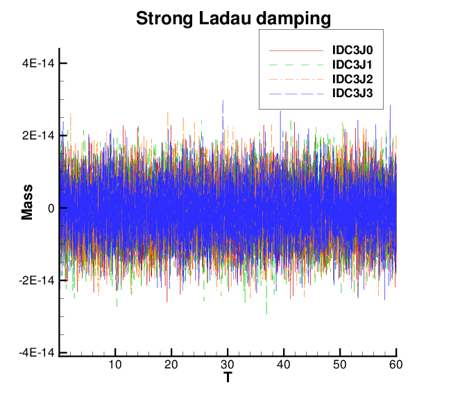
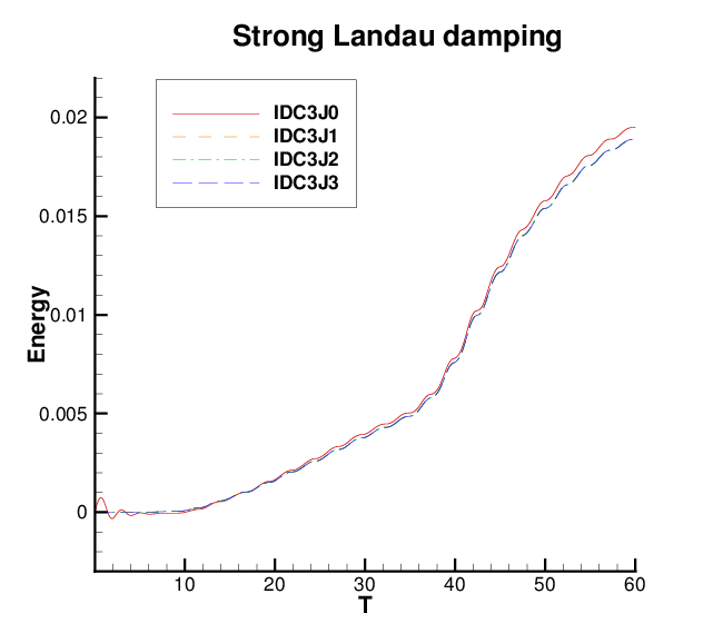
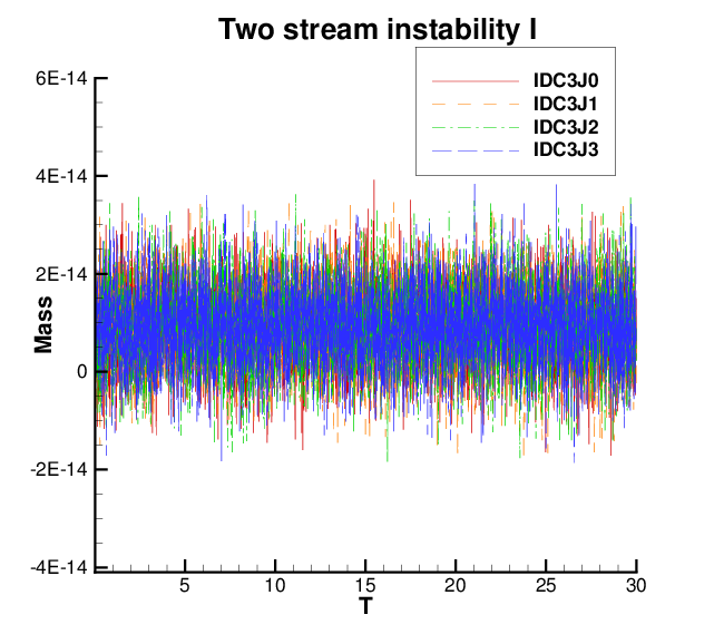
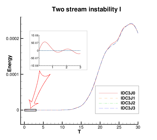
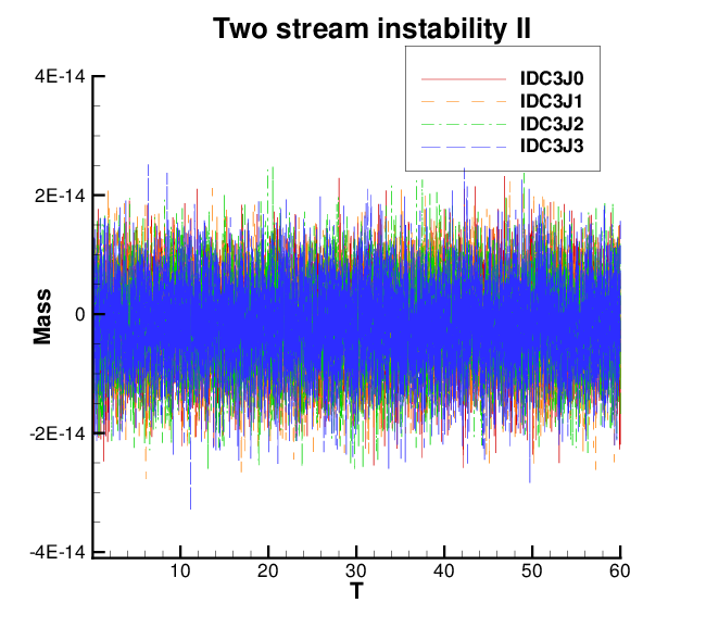
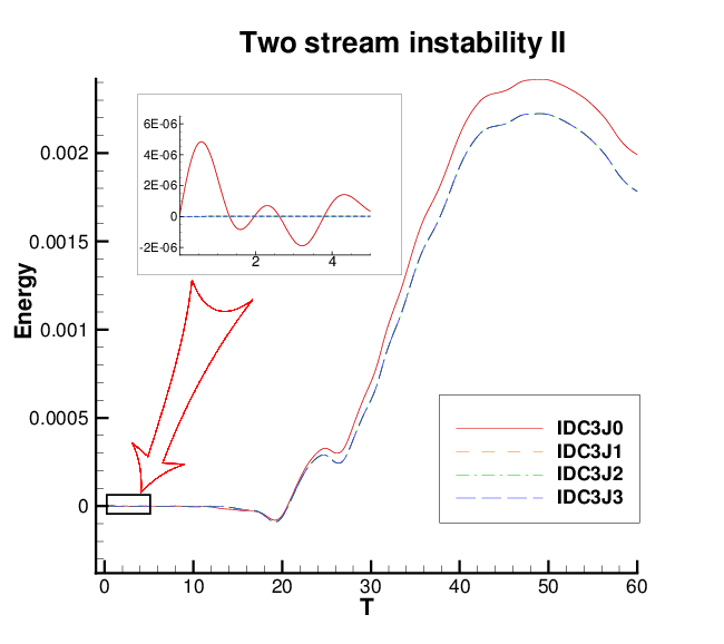
Figure 5.1: The time evolution of the relative deviation in total mass (left) and total energy (right). $N_{x}\times N_{v}=256\times 256$. $\text{CFL}=0.6$.

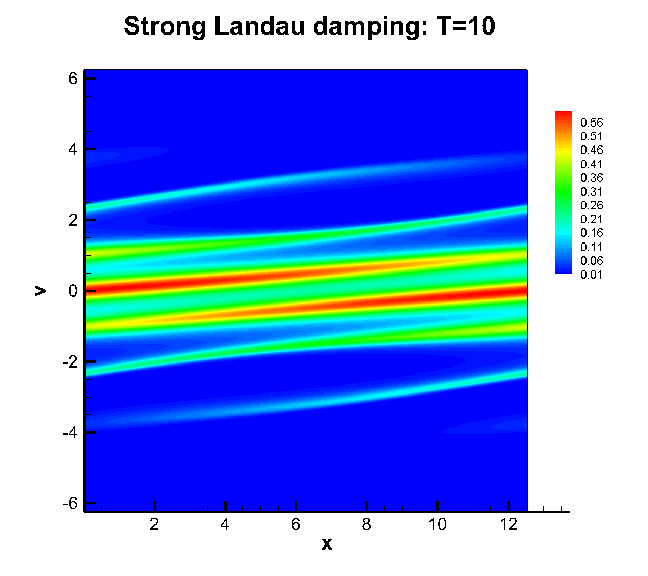
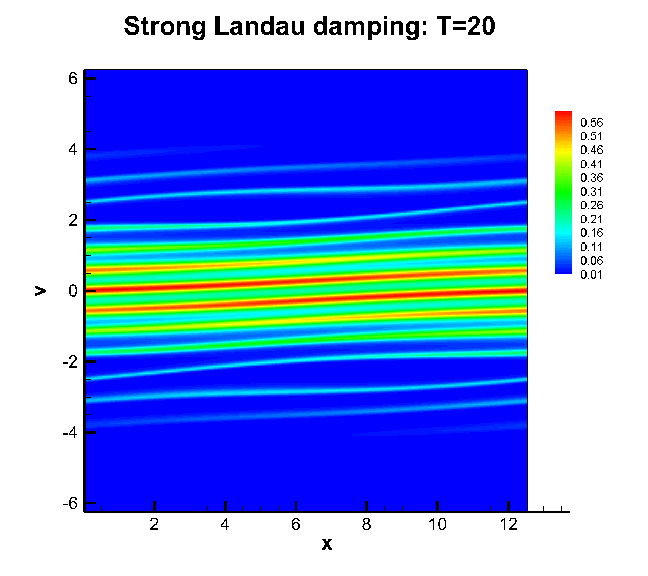
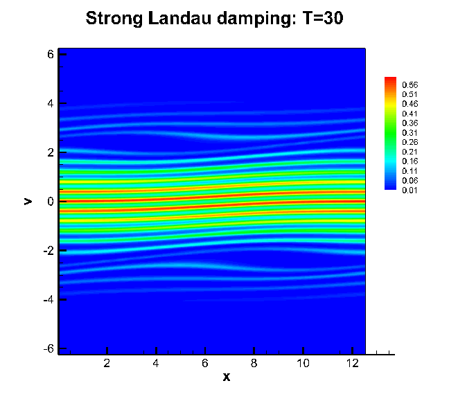
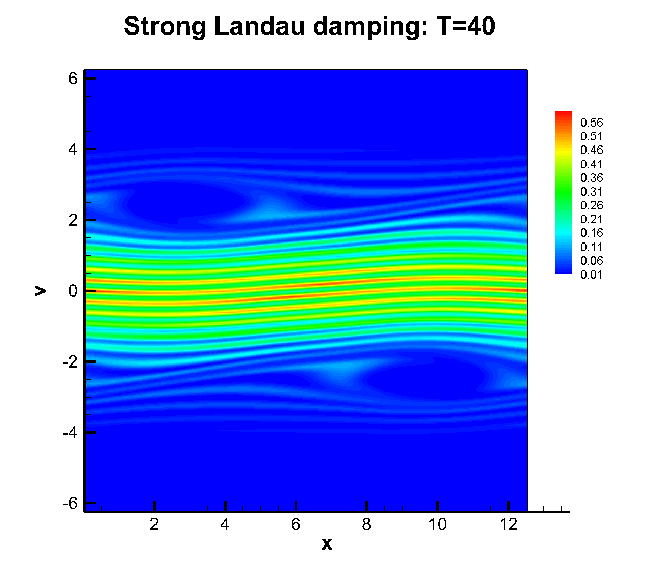
Figure 5.2: Contour plots of the numerical solutions for the strong Landau damping. $N_{x}\times N_{v}=256\times 256$. $\text{CFL}=0.6$. IDC3J3.

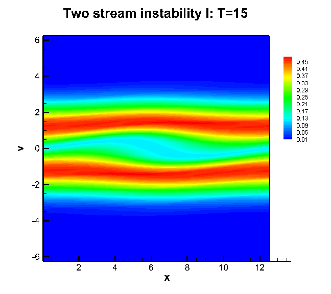
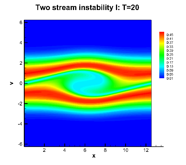
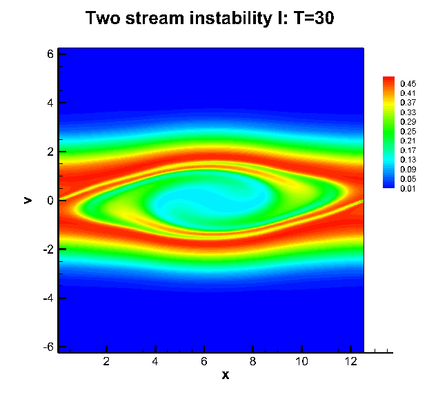
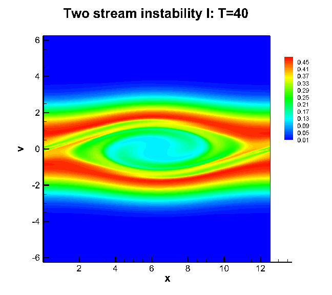
Figure 5.3: Contour plots of the numerical solutions for the two stream instability i@. $N_{x}\times N_{v}=256\times 256$. $\text{CFL}=0.6$. IDC3J3.

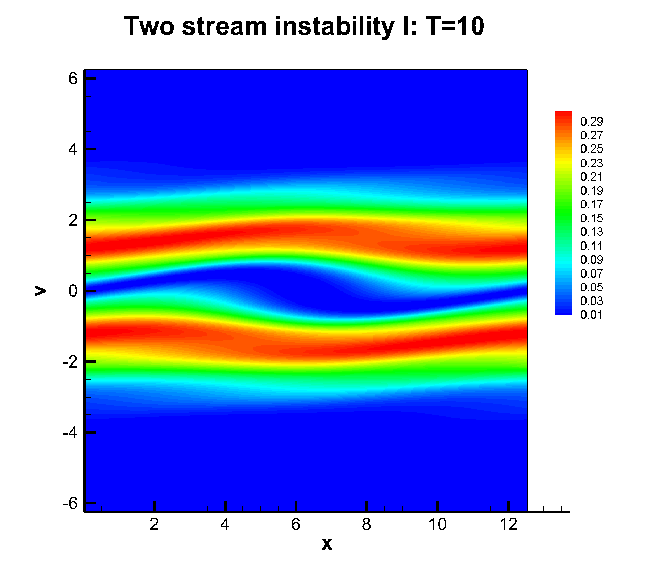
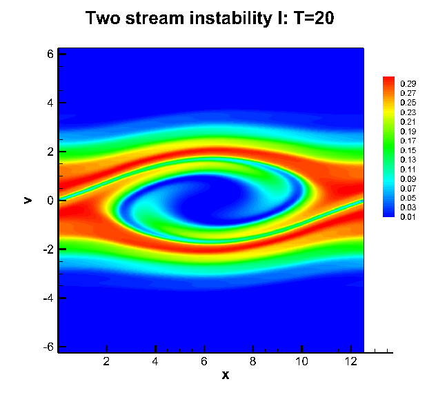
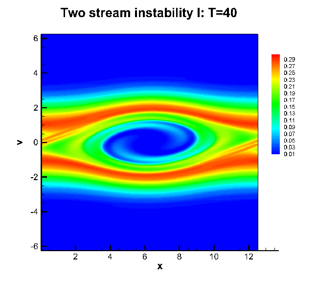
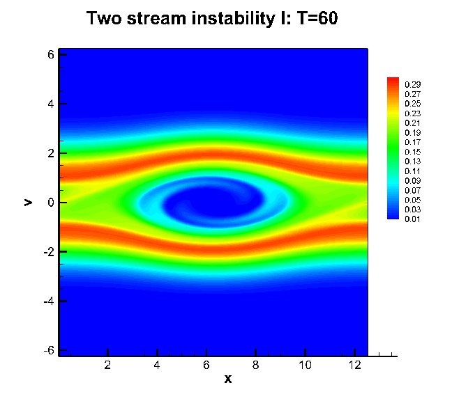
Figure 5.4: Contour plots of the numerical solutions for the two stream instability ii@. $N_{x}\times N_{v}=256\times 256$. $\text{CFL}=0.6$. IDC3J3.

5.2 2-D Guiding center Vlasov equation

We consider the guiding center model (3.17) with the initial condition [13]

$$\rho(x,y,0)=\sin(y)+0.015\cos(kx)$$

and periodic boundary conditions. We let $k=0.5$, thereby creating a Kelvin-Helmholtz instability. In the simulations, we set a mesh as $N_{x}\times N_{y}=128\times 128$. We use a third order SL finite difference WENO scheme as a base scheme to achieve third order spatial accuracy. In Figure 5.5 (top), we report the contour plots of numerical solutions at time $T=40$ for the first order splitting scheme (IDC3J0) and the third order scheme (IDC3J2) with $\text{CFL}=0.67$. A noticeable difference is observed. In Figure 5.6 (left), 1-D cuts of the numerical solutions at $y=\pi$ are plotted. The reference solution is computed by IDC3J2 with $\text{CFL}=0.05$. It can be observed that the numerical solution obtained by IDC3J2 with $\text{CFL}=0.67$ qualitatively matches the reference. However, a significant difference between the numerical solution obtained by the first order scheme and the reference solution is observed. Then we reduce the CFL number to 0.05 for the first order splitting scheme. The 2-D contour plot by the first order scheme approximately matches the reference by IDC3J2, see Figure 5.5 (bottom). A more precise match is also observed when the 1-D cuts of the numerical solutions are compared. The presented numerical evidence shows better performance from higher order numerical schemes in time. Note that the continuous guiding center model (3.17) preserves the $L^{2}$ norms of $\rho$ (enstrophy) and the $L^{2}$ norms of $\mathbf{E}$ (energy), i.e.:

$$\frac{d}{dt}\|\rho(t)\|_{L^{2}}=\frac{d}{dt}\|\mathbf{E}(t)\|_{L^{2}}=0.$$

We track the relative deviations of these invariants numerically as a measurement of the quality of numerical schemes. In Figure 5.7, the time evolutions of the enstrophy and the energy for the first order splitting scheme (IDC3J0), the second order scheme (IDC3J1) and the third order scheme (IDC3J2) are reported. It is observed that these quantities are better preserved by higher order schemes in time. Also note that little difference can be observed between the IDC3J1 and IDC3J2 solutions. In this case, the spatial error may dominate.

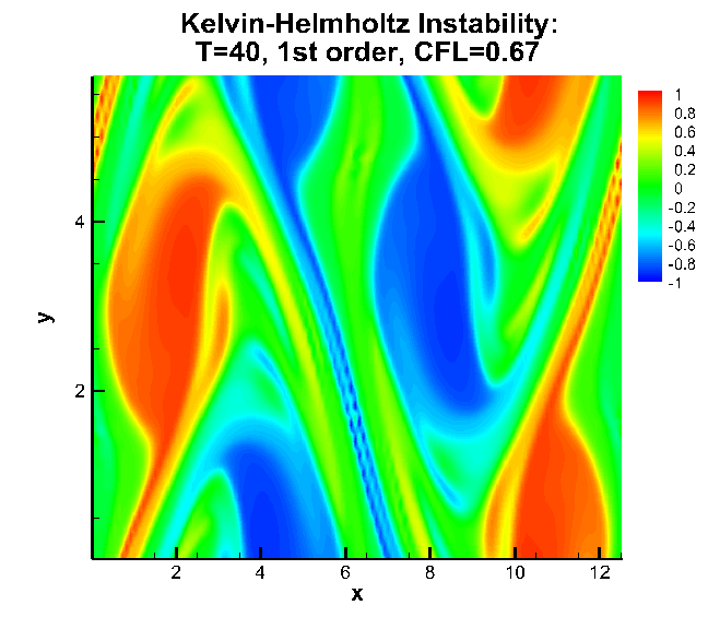
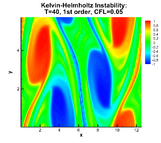
Figure 5.5: Contour plots of the numerical solutions for the Kelvin-Helmholtz instability. $N_{x}\times N_{y}=128\times 128$. $\text{CFL}=0.67$ (top) and $\text{CFL}=0.05$ (bottom) at $T=40$. First order scheme (IDC3J0) (left); Third order scheme (IDC3J2) (right).

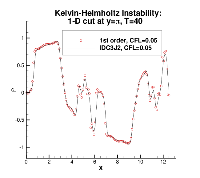
Figure 5.6: 1-D cuts of the numerical solutions at $y=\pi$ for the Kelvin-Helmholtz instability. $N_{x}\times N_{y}=128\times 128$. $T=40$. $\text{CFL}=0.67$ (left); $\text{CFL}=0.05$ (right). The reference solution is computed by IDC3J2 with $\text{CFL}=0.05$.

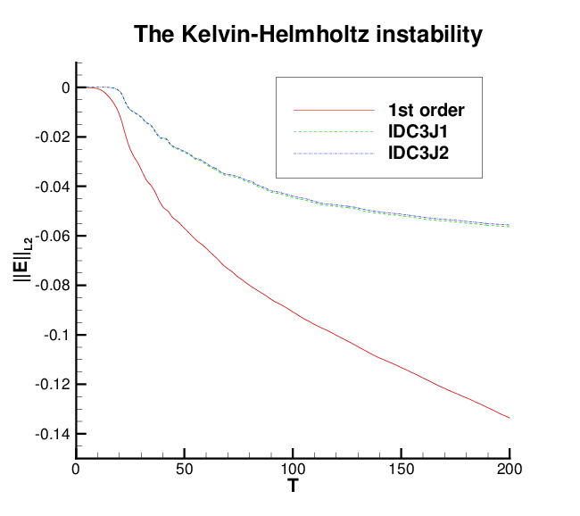
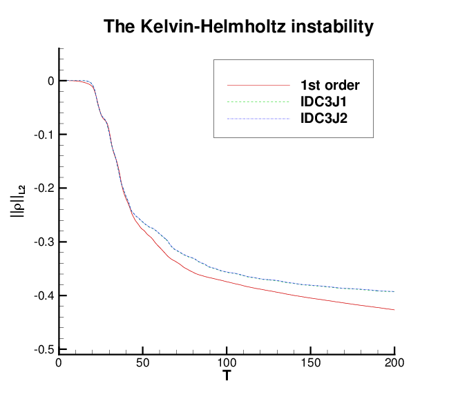
Figure 5.7: The Kelvin-Helmholtz instability. The time evolutions of the energy $\|\mathbf{E}\|_{L^{2}}$ (left) and the enstrophy $\|\rho\|_{L^{2}}$ (right). $N_{x}\times N_{y}=128\times 128$. $\text{CFL}=0.67$.

5.3 2-D incompressible Euler equations

We consider 2-D incompressible Euler equations in the vorticity stream-function formulation as follows

$$\omega_{t}+\nabla\cdot({\bf u}\omega)=0,\quad x\in[0,2\pi],\quad y\in[0,2\pi].$$ (5.4)

Here ${\bf u}=\nabla^{\perp}\Phi=(-\Phi_{y},\Phi_{x})$, where $\Phi$ is solved from the Poisson’s equation. We note that equation (5.4) is in the same form as the 2-D guiding center Vlasov equation (3.17). We first test the accuracy of the scheme with the following initial conditions:

$$\omega(x,y,t=0)=-2\sin(x)\sin(y),$$

and periodic boundary conditions. Note that the exact solution is identical to the initial condition. We use this example to check the order of accuracy of our proposed scheme when the IDC framework is adopted to correct the splitting error. In the simulation, we fix the spatial mesh as $N_{x}\times N_{y}=300\times 300$ and compute the numerical solutions with different CFLs. We evolve the solutions up to time $T=1$. In Table 5.6, we report the $L^{1}$ error and orders of accuracy for the first order splitting scheme (IDC3J0), the second order scheme (IDC3J1) and the third order scheme (IDC3J2). Expected orders of accuracy are observed. Note that third order convergence is not clearly observed for IDC3J2 when the CFL numbers are relatively small (CFL$\leq 0.5$). In this case, the spatial error begins to dominate when the numerical error is around $9.00E-9$. The $L^{1}$ error for IDC3J2 with $\text{CFL}=0.01$ is $9.31E-09$. We remark that there is a certain range of CFL numbers (which could be a very small interval), related to the spatial resolution and accuracy, where the temporal order of accuracy can be numerically observed. Above that range, the scheme is either numerically unstable or the order of convergence can not be observed yet; below that range, the spatial error could dominate, with which the temporal order of convergence can no longer be observed.

Table 5.6: 2-D incompressible Euler equation. A third order SL WENO scheme coupled in the IDC framework. $L^{1}$ norms of errors and orders of accuracy. $N_{x}\times N_{y}=300\times 300$. $T=1$.

	IDC3J0		IDC3J1		IDC3J2
CFL	$L^{1}$ error	$L^{1}$ order	$L^{1}$ error	$L^{1}$ order	$L^{1}$ error	$L^{1}$ order
0.67	2.16E-03	–	8.89E-06	–	5.39E-08	–
0.62	2.00E-03	0.97	7.63E-06	1.97	4.26E-08	3.02
0.57	1.83E-03	1.02	6.43E-06	2.03	3.29E-08	3.07
0.52	1.67E-03	0.99	5.36E-06	1.99	2.51E-08	2.96
0.47	1.51E-03	1.01	4.37E-06	2.01	1.92E-08	2.63

We then consider two benchmark tests. One is shear flow with the initial condition given by:

$$\left\{\begin{array}[]{ll}\displaystyle\omega(x,y,0)=\delta\cos(x)-\frac{1}{\rho}\text{sech}^{2}((y-\pi/2)/\rho),&\text{if}\quad y\leq\pi,\\[14.22636pt] \displaystyle\omega(x,y,0)=\delta\cos(x)+\frac{1}{\rho}\text{sech}^{2}((3\pi/2-y)/\rho),&\text{if}\quad y>\pi,\end{array}\right.$$ (5.5)

where $\delta=0.05$ and $\rho=\frac{\pi}{15}$. The other is a vortex patch, and the initial condition is given by:

$$\left\{\begin{array}[]{ll}\omega(x,y,0)=-1,&\displaystyle\text{if}\quad(x,y)\in[\frac{\pi}{2},\frac{3\pi}{2}]\times[\frac{\pi}{4},\frac{3\pi}{4}],\\[14.22636pt] \omega(x,y,0)=1,&\displaystyle\text{if}\quad(x,y)\in[\frac{\pi}{2},\frac{3\pi}{2}]\times[\frac{5\pi}{4},\frac{7\pi}{4}],\\[14.22636pt] \omega(x,y,0)=0,&\text{ otherwise}.\end{array}\right.$$ (5.6)

In the simulations for the shear flow, we set the mesh as $N_{x}\times N_{y}=128\times 128$. A third order SL WENO scheme [30] is used to obtain solutions in the IDC prediction step. In Figure 5.8, we report the contours of the numerical solution at time $T=8$ for the first order splitting scheme and IDC3J2. Little difference can be observed from the contour plot. To better see the difference, in Figure 5.9, 1-D cuts at $x=\pi$ of the numerical solution are reported. We use the solution computed by IDC3J2 with $\text{CFL}=0.05$ as a reference. It is observed that the solution by IDC3J2 with $\text{CFL}=0.67$ matches the reference solution very well, whereas there is a noticeable difference between the solution by the first order scheme with $\text{CFL}=0.67$ and the reference. Then we reduce the CFL to 0.05 for the first order scheme and the corresponding temporal error is reduced. A more precise match is observed. The comparison shows the better performance of coupling the high order IDC methods to correct low order splitting errors. For the vortex patch test, we set the mesh size as $N_{x}\times N_{y}=256\times 256$. Figure 5.10 gives the numerical solutions at time $T=5$ (top) and $T=10$ (bottom) for the first order scheme (IDC3J0) (left) and IDC3J2 (right). The solution structure is observed to be slightly better resolved when the high order IDC framework is used.

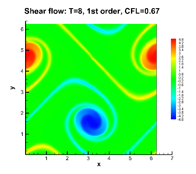
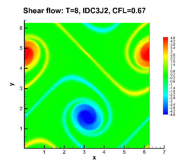
Figure 5.8: Contour plots of the numerical solutions for the shear flow test. $N_{x}\times N_{y}=128\times 128$. $\text{CFL}=0.67$ at $T=8$. First order scheme (IDC3J0) (left); Third order scheme (IDC3J2) (right).

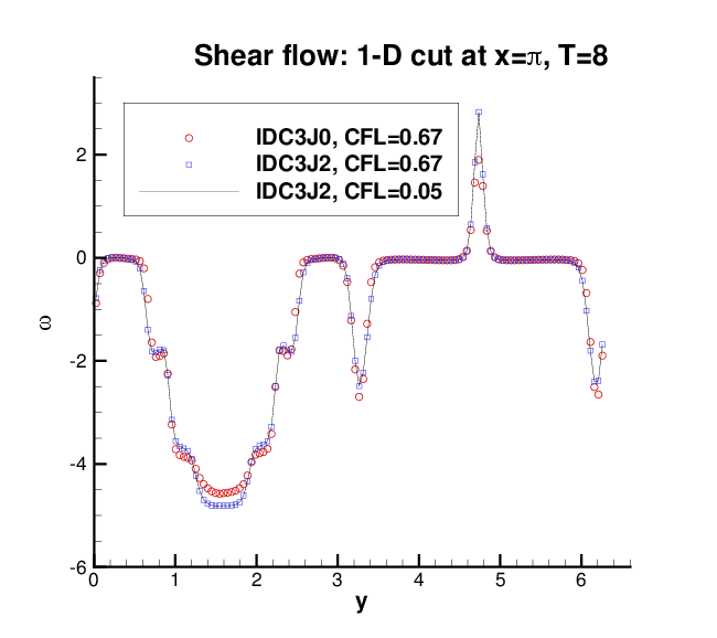
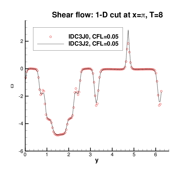
Figure 5.9: 1-D cuts of the numerical solutions at $x=\pi$ for the shear flow test. $N_{x}\times N_{y}=128\times 128$. $T=8$. $\text{CFL}=0.67$ (left); $\text{CFL}=0.05$ (right). The reference solution is computed by IDC3J2 with $\text{CFL}=0.05$.

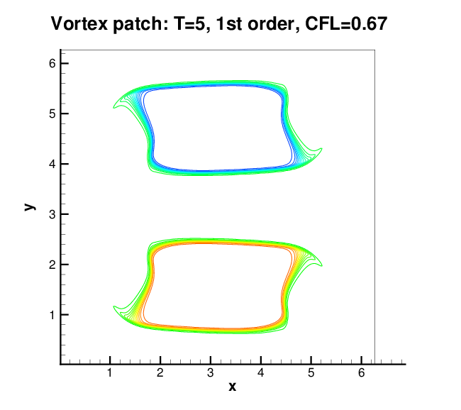
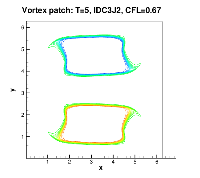
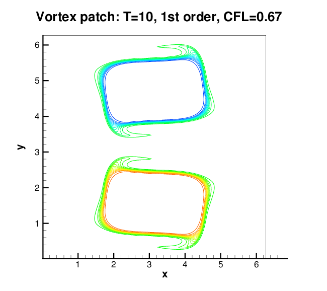
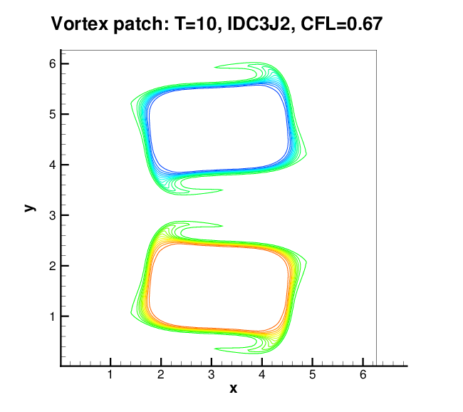
Figure 5.10: Contour plots of the numerical solutions for the vortex patch test. $N_{x}\times N_{y}=256\times 256$. $\text{CFL}=0.67$ at $T=5$ (top) and $T=10$ (bottom). First order scheme (IDC3J0) (left); Third order scheme (IDC3J2) (right). 30 equally spaced contours from -1.1 to 1.1.

6 Conclusion

In this paper, we proposed numerical methods that are high order in space and in time for Vlasov simulations. The proposed methods couple the SL finite difference WENO scheme with the IDC framework: we adopt the dimensional splitting SL WENO scheme as a base scheme to get a predicted solution in IDC, and the low order dimensional splitting error is iteratively reduced by solving the error equations again in a dimensional splitting fashion in the correction steps in IDC. We extended the scheme to solve the guiding center Vlasov equation and the two dimensional incompressible flow in vorticity stream-function formulation. A collection of numerical experiments demonstrate great performance of the proposed high order scheme in resolving solutions’ structures, even in the long term. Unfortunately, the IDC framework renders some CFL time step restriction, despite the SL evolution mechanism in the prediction and correction steps of IDC. We quantify such CFL restrictions via Fourier analysis for several high order methods that we used in simulations. Another potential difficulty is the implementation of boundary conditions in a high order manner for problems with non-periodic boundary conditions. These are subject to future investigations.

Acknowledgement. The authors thank Dr. Matt Causley for many helpful comments and suggestions.

References

- [1] M. Begue, A. Ghizzo, P. Bertrand, E. Sonnendrücker, and O. Coulaud, Two-dimensional semi-Lagrangian Vlasov simulations of laser–plasma interaction in the relativistic regime, J. Plasma Phys., 62 (1999), pp. 367–388.
- [2] N. Besse and E. Sonnendrücker, Semi-Lagrangian schemes for the Vlasov equation on an unstructured mesh of phase space, J. Comput. Phys., 191 (2003), pp. 341–376.
- [3] C. K. Birdsall and A. B. Langdon, Plasma Physics Via Computer Simulaition, CRC Press, 2005.
- [4] A. Bourlioux, A. T. Layton, and M. L. Minion, High-order multi-implicit spectral deferred correction methods for problems of reactive flow, J. Comput. Phys., 189 (2003), pp. 651–675.
- [5] J. A. Carrillo and F. Vecil, Nonoscillatory interpolation methods applied to Vlasov-based models, SIAM J. Sci. Comput., 29 (2007), pp. 1179–1206.
- [6] C. Cheng and G. Knorr, The integration of the Vlasov equation in configuration space, J. Comput. Phys., 22 (1976), pp. 330–351.
- [7] Y. Cheng, A. Christlieb, and X. Zhong, Energy-conserving discontinuous Galerkin methods for the Vlasov–Ampère system, arXiv preprint, arXiv:1306.0931, (2013).
- [8] Y. Cheng, I. M. Gamba, and P. J. Morrison, Study of conservation and recurrence of Runge–Kutta discontinuous Galerkin schemes for Vlasov–Poisson systems, J. Sci. Comput., (2012), pp. 1–31.
- [9] A. Christlieb, Y. Liu, and Z. Xu, High order operator splitting methods based on an integral deferred correction framework, submitted, (2013).
- [10] A. Christlieb, C. Macdonald, and B. Ong, Parallel high-order integrators, SIAM J. Sci. Comput., 32 (2010), pp. 818–835.
- [11] A. Christlieb, B. Ong, and J.-M. Qiu, Comments on high order integrators embedded within integral deferred correction methods, Comm. Appl. Math. Comput. Sci, 4 (2009), pp. 27–56.
- [12] A. Christlieb, B. Ong, and J.-M. Qiu, Integral Deferred Correction Methods constructed with high order Runge–Kutta integrators, Math. Comp., 79 (2010), pp. 761–783.
- [13] N. Crouseilles, M. Mehrenberger, and E. Sonnendrücker, Conservative semi-Lagrangian schemes for Vlasov equations, J. Comput. Phys., 229 (2010), pp. 1927–1953.
- [14] A. Dutt, L. Greengard, and V. Rokhlin, Spectral deferred correction methods for ordinary differential equations, BIT, 40 (2000), pp. 241–266.
- [15] F. Filbet and E. Sonnendrücker, Comparison of Eulerian Vlasov solvers, Comput. Phys. Commun., 150 (2003), pp. 247–266.
- [16] F. Filbet, E. Sonnendrücker, and P. Bertrand, Conservative numerical schemes for the Vlasov equation, J. Comput. Phys., 172 (2001), pp. 166–187.
- [17] R. Frank and C. W. Ueberhuber, Iterated defect correction for differential equations. I. Theoretical results, Computing, 20 (1978), pp. 207–228.
- [18] W. Guo, R. D. Nair, and J.-M. Qiu, A conservative semi-Lagrangian discontinuous Galerkin scheme on the cubed-sphere, Mon. Wea. Rev., (2013).
- [19] W. Guo and J.-M. Qiu, Hybrid semi-Lagrangian finite element-finite difference methods for the Vlasov equation, J. Comput. Phys., 234 (2013), pp. 108–132.
- [20] E. Hairer, C. Lubich, and G. Wanner, Geometric numerical integration, vol. 31 of Springer Series in Computational Mathematics, Springer-Verlag, Berlin, second ed., 2006. Structure-preserving algorithms for ordinary differential equations.
- [21] E. Hansen and A. Ostermann, High order splitting methods for analytic semigroups exist, BIT, 49 (2009), pp. 527–542.
- [22] R. Heath, I. Gamba, P. Morrison, and C. Michler, A discontinuous Galerkin method for the Vlasov–Poisson system, J. Comput. Phys., 231 (2012), pp. 1140–1174.
- [23] R. W. Hockney and J. W. Eastwood, Computer simulation using particles, CRC Press, 2010.
- [24] F. Huot, A. Ghizzo, P. Bertrand, E. Sonnendrücker, and O. Coulaud, Instability of the time splitting scheme for the one-dimensional and relativistic Vlasov–Maxwell system, J. Comput. Phys., 185 (2003), pp. 512–531.
- [25] A. T. Layton and M. L. Minion, Conservative multi-implicit spectral deferred correction methods for reacting gas dynamics, J. Comput. Phys., 194 (2004), pp. 697–715.
- [26] T. Nakamura, R. Tanaka, T. Yabe, and K. Takizawa, Exactly conservative semi-Lagrangian scheme for multi-dimensional hyperbolic equations with directional splitting technique, J. Comput. Phys., 174 (2001), pp. 171–207.
- [27] T. Nakamura and T. Yabe, Cubic interpolated propagation scheme for solving the hyper-dimensional Vlasov–Poisson equation in phase space, Comput. Phys. Commun., 120 (1999), pp. 122–154.
- [28] V. Pereyra, Iterated deferred corrections for nonlinear operator equations, Numer. Math., 10 (1967), pp. 316–323.
- [29] J.-M. Qiu and A. Christlieb, A Conservative high order semi-Lagrangian WENO method for the Vlasov equation, J. Comput. Phys., 229 (2010), pp. 1130–1149.
- [30] J.-M. Qiu and C.-W. Shu, Conservative high order semi-Lagrangian finite difference WENO methods for advection in incompressible flow, J. Comput. Phys., 230 (2011), pp. 863–889.
- [31] , Conservative semi-Lagrangian finite difference WENO formulations with applications to the Vlasov equation, Commun. Comput. Phys., 10 (2011), pp. 979–1000.
- [32] , Positivity preserving semi-Lagrangian discontinuous Galerkin formulation: theoretical analysis and application to the Vlasov-Poisson system, J. Comput. Phys., 230 (2011), pp. 8386–8409.
- [33] J. Rossmanith and D. Seal, A positivity-preserving high-order semi-Lagrangian discontinuous Galerkin scheme for the Vlasov-Poisson equations, J. Comput. Phys., 227 (2011), pp. 9527–9553.
- [34] J. Schaeffer, Higher order time splitting for the linear Vlasov equation, SIAM J. Numer. Anal., 47 (2009), pp. 2203–2223.
- [35] E. Sonnendrücker, J. Roche, P. Bertrand, and A. Ghizzo, The semi-Lagrangian method for the numerical resolution of the Vlasov equation, J. Comput. Phys., 149 (1999), pp. 201–220.
- [36] A. Staniforth and J. Cote, Semi-Lagrangian integration schemes for atmospheric models–a review, Mon. Wea. Rev., 119 (1991), pp. 2206–2223.
- [37] H. J. Stetter, The defect correction principle and discretization methods, Numer. Math., 29 (1978), pp. 425–443.
- [38] G. Strang, On the construction and comparison of difference schemes, SIAM J. Numer. Anal., 5 (1968), pp. 506–517.
- [39] T. Umeda, M. Ashour-Abdalla, and D. Schriver, Comparison of numerical interpolation schemes for one-dimensional electrostatic Vlasov code, J. Plasma Phys., 72 (2006), pp. 1057–1060.
- [40] J. P. Verboncoeur, Particle simulation of plasmas: review and advances, Plasma Phys. Contr. F., 47 (2005), pp. A231 –A260.
- [41] Y. Xia, Y. Xu, and C.-W. Shu, Efficient time discretization for local discontinuous Galerkin methods, Discrete Contin. Dyn. Syst. Ser. B, 8 (2007), pp. 677–693.
- [42] H. Yoshida, Construction of higher order symplectic integrators, Phys. Lett. A, 150 (1990), pp. 262–268.
- [43] T. Zhou, Y. Guo, and C.-W. Shu, Numerical study on Landau damping, Phys. D, 157 (2001), pp. 322–333.