A Ground-based Optical Transmission Spectrum of WASP-6b

Abstract

We present a ground based optical transmission spectrum of the inflated sub-Jupiter mass planet WASP-6b. The spectrum was measured in twenty spectral channels from 480 nm to 860nm using a series of 91 spectra over a complete transit event. The observations were carried out using multi-object differential spectrophotometry with the IMACS spectrograph on the Baade telescope at Las Campanas Observatory. We model systematic effects on the observed light curves using principal component analysis on the comparison stars, and allow for the presence of short and long memory correlation structure in our Monte Carlo Markov Chain analysis of the transit light curves for WASP-6. The measured transmission spectrum presents a general trend of decreasing apparent planetary size with wavelength and lacks evidence for broad spectral features of Na and K predicted by clear atmosphere models. The spectrum is consistent with that expected for scattering that is more efficient in the blue, as could be caused by hazes or condensates in the atmosphere of WASP-6b. WASP-6b therefore appears to be yet another massive exoplanet with evidence for a mostly featureless transmission spectrum, underscoring the importance that hazes and condensates can have in determining the transmission spectra of exoplanets.

1. Introduction

Due to their fortitious geometry transiting exoplanets allow the determination of physical properties that are inaccesible or hard to reach for non-transiting system. One of the most exciting possibilities enabled by the transting geometry is to measure atmospheric properties of exoplanets without the need to resolve them from their parent star through the technique of transmission spectroscopy. In this technique, the atmospheric opacity at the planet terminator is probed by measuring the planetary size via transit light curve observations at different wavelengths. The measurable quantity is the planet-to-star radius ratio as a function of wavelength, $(R_{p}/R_{*})(\lambda)\equiv k(\lambda)$, and is termed the transmission spectrum. The measurement of a transmission spectrum is a challenging one, with one atmospheric scale height $H$ translating to a signal of order $2Hk\approx 10^{-4}$ for hot Jupiters (e.g., Brown, 2001). The requirements on precision favour exoplanets with large atmospheric scale heights, large values of $k$ (e.g., systems transiting M dwarfs) and orbiting bright targets due to the necessity of acquiring a large number of photons to reach the needed precision.

The first successful measurement by transmission spectroscopy was the detection with the Hubble Space Telescope (HST) of absorption by Na I in the hot Jupiter HD 209458b (Charbonneau et al., 2002). The signature of Na was 2–3 times weaker than expected from clear atmosphere models, providing the first indications that condensates can play an important role in determining the opacity of their atmospheres as seen in transmission (e.g., Fortney, 2005, and references therein). Subsequent space based studies have concentrated largely on the planets orbiting the stars HD 209458 and HD 189733 due to the fact that they are very bright stars, and therefore allow the collection of large number of photons even with the modest aperture of space based telescopes. A recent study of all the transmission spectra available for HD 189733, spanning the range from 0.32 to 24 $\mu$m, points to a spectrum dominated by Rayleigh scattering over the visible and near infra-red range with the only detected feature being a narrow resonance line of Na (Pont et al., 2013). For HD 209458, Deming et al. (2013) present new WFC3 data combined with previous STIS data (Sing et al., 2008), resulting in a transmission spectrum spanning the wavelength range 0.3 to 1.6 $\mu$m. They conclude that the broad features of the spectrum are dominated by haze and/or dust opacity. In both cases the spectra are different from those predicted by clear atmosphere models that do not incorporate condensates.

In order to further our understanding of gas giant atmospheres it is necessary to build a larger sample of systems with measured transmission spectra. Hundreds of transiting exoplanets, mostly hot gas giants, have been discovered by ground based surveys such as HATNet (Bakos et al., 2004), WASP (Pollacco et al., 2006), KELT (Pepper et al., 2007), XO (McCullough et al., 2005), TRES (Alonso et al., 2004) and HATSouth (Bakos et al., 2013), with magnitudes within reach of the larger collecting areas afforded by ground based telescopes but often too faint for HST. The ground based observations have to contend with the atmosphere and instruments lacking the space-based stability of HST, but despite these extra hurdles the pace of ground-based transmission spectra studies is steadily increasing. Following the ground-based detection of Na I in HD189733b (Redfield et al., 2008) and confirmation of Na I in HD209358b (Snellen et al., 2008), Na I has been additionally reported from the ground in WASP-17b (Wood et al., 2011; Zhou & Bayliss, 2012) and XO-2b (Sing et al., 2012). K I has been detected in XO-2b (Sing et al., 2011a) and the highly eccentric exoplanet HD80606b (Colón et al., 2012). All of these studies have used high resolution spectroscopy or narrow band photometry to specifically target resonant lines of alkali elements. Recently, a detection of H$\alpha$ has been reported from the ground for HD 189733b (Jensen et al., 2012), complementing previous space-based detection of Ly$\alpha$ and atomic lines in the UV with HST for HD 189733b and HD 209358b (Vidal-Madjar et al., 2003, 2004; Lecavelier Des Etangs et al., 2010).

Differential spectrophotometry using multi-object spectrographs offer an attractive means to obtain transmission spectra given the possibility of using comparison stars to account for the various systematic effects that affect the spectral time series obtained. Using such spectrograps, transmission spectra in the optical have been obtained for GJ 1214b (Bean et al., 2011, 610-1000 nm with VLT/FORS) and recently for WASP29-b (Gibson et al., 2013, 515-720 nm with Gemini/GMOS), with both studies finding featureless spectra. In the near infrared Bean et al. (2013) present a transmission spectrum in the range 1.25 to 2.35 $\mu$m for WASP-19b, using MMIRS on Magellan. In this work we present an optical transmission spectrum of another planet, WASP-6 b, an inflated sub Jupiter mass ($0.504M_{J}$) planet orbiting a $V=11.9$ G dwarf (Gillon et al., 2009), in the in the range 471–863 nm.

2. Observations

The transmission spectrum spectrum of WASP-6b was obtained performing multi-object differential spectrophotometry with the Inamori-Magellan Areal Camera & Spectrograph (IMACS, Dressler et al., 2011) mounted on the 6.5m Baade telescope at Las Campanas Observatory. A series of 91 spectra of WASP-6 and a set of comparison stars were obtained during a transit of the hot Jupiter WASP-6b in October 03 2010 with the f/2 camera of IMACS, which provides an unvignetted circular field of view of radius $r\approx 12$ arcmin. The large field of view makes IMACS a very attractive instrument for multi-object differential spectrophotometry as it allows to search for suitable comparison stars that have as much as possible similar magnitude and colors as the target star. The median cadence of our observations was 224 sec, and the exposure time was set to 140 sec, except for the first eight exposures when we were tuning the exposure level and whose exposure times were $\{30,120,150,150,150,130,130,130\}$ sec. The count level of the brightest pixel in the spectrum of WASP-6 was $\approx$ 43000 ADU, i.e. $\approx$ 65% of the saturation level. In addition to WASP-6 we observed 10 comparison stars of comparable magnitude, seven of which had the whole wavelength range of interest ($\approx 4700-8600\ \text{\AA}$) recorded in the CCD with enough signal-to-noise. The seven comparison stars we used are listed in Table 1. The integrated counts over the wavelength range of interest for the spectrum of WASP-6 was typically $\approx 3.6\times 10^{8}$ electrons, giving a Poisson noise limit for the white-light light curve of $\approx 0.06$ mmag. Each star was observed through a $10\times 10$ arcsec² slit in order to avoid the adverse effects of variable slit losses. We used the 300-l+17 grating as dispersing element, which gave us a seeing-dependent resolution $\Delta\lambda$ which was $\approx$ $5\ \text{\AA}$ under $0.7$ arcsec seeing and a dispersion of $1.34\text{\AA}$ per pixel. In addition to the science mask, we obtained HeNeAr arc lamps through a mask that had slits at the same position as the science mask but with slit widths in the spectral direction of $0.7$ arcsec. Observing such masks is necessary in order to produce well defined lines that are then used to define the wavelength solution.

Table 1List of comparison stars

2MASS identifier
2MASS-23124095-2243232
2MASS-23124836-2252099
2MASS-23124448-2253190
2MASS-23124428-2256403
2MASS-23114068-2248130
2MASS-23113937-2250334
2MASS-23114820-2256592

The extracted spectra of WASP-6 and the seven comparison stars we used are shown for a typical exposure in Figure 1. The conditions throughout the night were variable. The raw light curves constructed with the integrated counts over the whole spectral range for WASP-6 and the comparison stars are shown as a function of time in Figure 2. Besides the variation due to varying airmass (and the transit for WASP-6), there were periods with strongly varying levels of transparency concentrated in the period of time 0–2 hrs after mid-transit. The seeing was in the range $\approx$ 0.6–0.8″. In order to maintain good sampling of the PSF in the spatial direction we defocused the telescope slightly in the periods of best seeing. Changes in seeing and transparency left no noticeable traces in the final light curves.

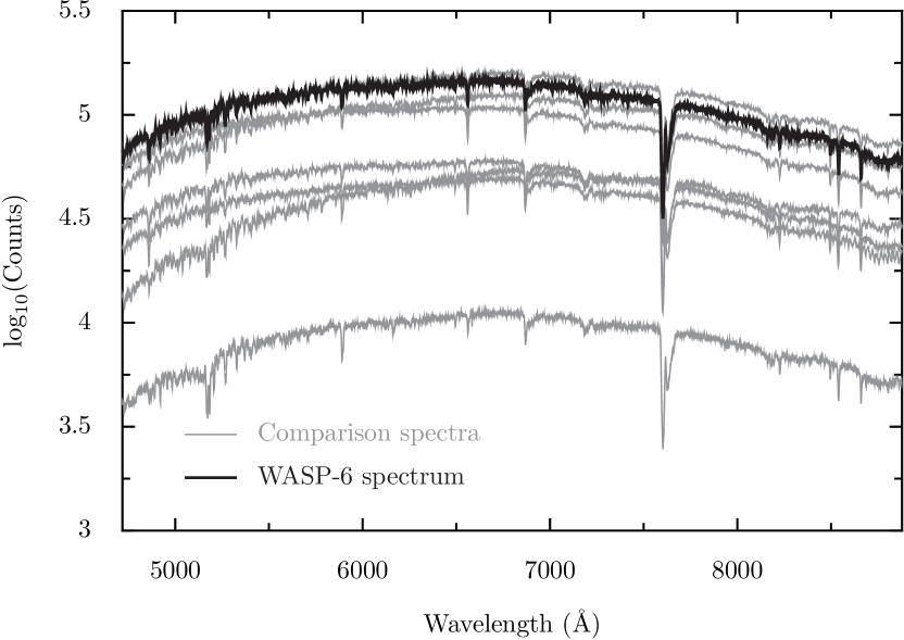
Figure 1.— Extracted spectra for WASP-6 and the seven comparison stars used in this work for a typical exposure.

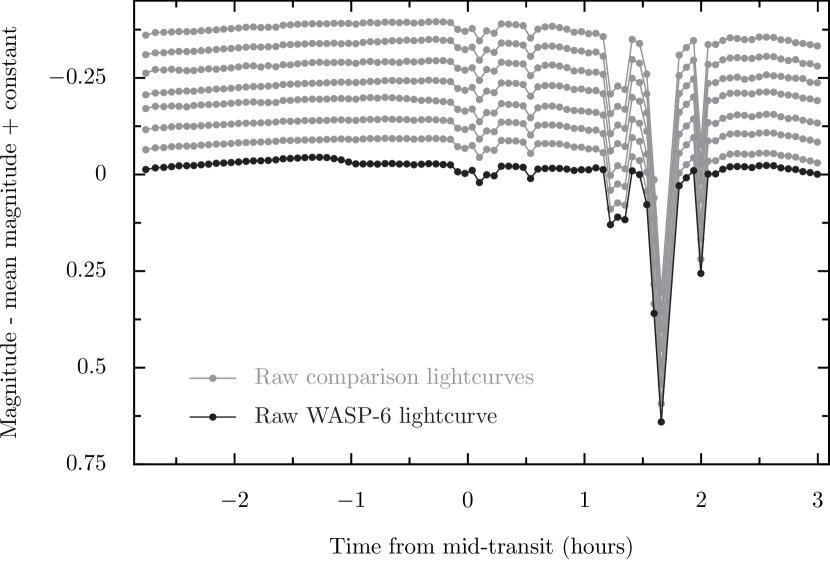
Figure 2.— Raw light curves for WASP-6 and seven comparison stars used in this work as a function of time.

3. Data reduction

3.1. Background and sky substraction

After substracting the median value of the overscan region to every image, an initial trace of each spectrum was obtained by calculating the centroid of each row, which are perpendicular to the dispersion direction. Each row was then divided in three regions: a central region, which contains the bulk of the light of the star, a middle, on-slit region which is dominated by sky continuum and line emission, and an outer, out-of-slit region which contains a smooth background outside the slit arising from, e.g., scattered light. The middle and outer regions have components on each side of the spectrum. The outermost region was used to determine a smooth background that varies slowly along the dispersion direction. The median level was obtained in the outer regions on either side of the slit, and then a 3rd order polynomial was used to estimate the average background level as a function of pixel in the dispersion direction. This smooth background component was then subtracted from the central and middle regions. Then a Moffat function plus a constant level $c_{i}$ was fit robustly to each background subtracted row in those regions. The estimated $c_{i}$ (one per row), was then substracted from the central and middle regions in order to obtain a spectrum where only the stellar contribution remains. It is necessary to estimate the sky emission on a row-per-row basis as sky emission lines have a wide, box-shaped form with sharp boundaries due to the fact they fully illuminate the wide slit.

3.2. Fine tracing and spectrum extraction

The background and sky subtracted spectrum was traced by an algorithm that cross-correlates each slice perpendicular to the wavelength direction with a Gaussian in order to find the spectral trace. The centers of the trace were then fitted robustly with a fourth order polynomial. This new tracing procedure served as a double check for the centers obtained via the centroid method in the background and sky substraction part of the data reduction process; both methods gave traces consistent whith each other. With the trace in hand, the spectrum was extracted by using a simple extraction procedure, i.e. summing the flux on each row $\pm 15$ pixels form the trace position at that row. We also tried optimal extraction (Marsh, 1989), but it lead to additional systematic effects when analyzing the light curves, and in any case optimal extraction is not expected to give significant gains over simple extraction at the high signal-to-noise levels we are working with here. We also took spectroscopic flats at the begining of the night with a quartz lamp and reduced the data using both flat-fielded and non flat-fielded spectra. The results where consistent when using both alternate reductions, but the flat-fielded spectra showed higher dispersion in the final transmission spectrum. We therefore used the non flat-fielded spectra in the present work.

3.3. Wavelength calibration

The extracted spectra were calibrated using NeHeAr lamps taken at the start of the night. The wavelength solution was obtained by the following iterative procedure: pixel centers of lines with known wavelengths where obtained by fitting Gaussians to them, and then all the pixel centers, along with the known wavelengths of the lines were fitted by a 6th order Chebyshev polynomial. We checked the absolute deviation of each line from the fit, and removed the most deviant one from our sample, repeating the fit without it. This process was iterated, removing one line at a time, until a rms of less than 2000 m/s was obtained. The rms of the final wavelength solution was $\approx 1200$ m/s, using $27$ lines.

The procedure explained in the preceding paragraph served to wavelength calibrate the first spectrum of the night closest in time to the NeHeAr lamps. In order to measure and correct for wavelength shifts throughout the night, the first spectrum was cross-correlated with the subsequent ones in pixel-space in order to find the shifts in wavelength-space. If $\lambda_{t_{0},s}(p)$ is the wavelength solution at time $t_{0}$ (the beggining of the night) for star $s$ as a function of the pixel $p$, then the wavelength solution at time $t$ is just $\lambda_{t,s}(p+\delta p_{t,s})$, where $\delta p_{t,s}$ is the shift in pixel-space found by cross-correlating the spectrum of star $s$ taken at time $t_{0}$ with the one taken at time $t$. Finally, each spectrum was fitted with a b-spline in order to interpolate each of the spectra into a common wavelength grid with pixel size $0.75\text{\AA}$.

4. Modelling Framework

The observed signal of WASP-6 is perturbed with respect to its intrinsic shape, which we assume ideally to be a constant flux, $F$. This constant flux is multiplied by the transit signal, $f(t;\theta)$, which we describe parametrically using the formalism of Mandel & Agol (2002). In what follows $\theta$ represents the vector of transit parameters. The largest departure from this idealized model in our observations will be given by systematic effects arising from atmospheric and instrumental effects, which are assumed to act multiplicatively on our signals. We will model the logarithm of the observed flux, $L(t)$, as

$$L(t;\theta)=S(t)+\log_{{10}}f(t;\theta)+\log_{{10}}F+\epsilon(t),$$ (1)

where $S(t)$ represents the (multiplicative) perturbation to the star’s flux, which we’ll refer to in what follows as the perturbation signal, and $\epsilon(t)$ is a stochastic signal which represents the noise in our measurements (under the term noise we will also include potential variations of the star that are not accounted for in the estimate of the deterministic $S(t)$ and that can be modelled by a stochastic signal).

4.1. Modelling the perturbation signal

4.1.1 Estimation of Systematic Effects via Principal Component Analysis of the Comparison Stars

Each star in the field is affected by a different perturbation signal. However, these perturbation signals have in common that they arise from the same physical and instrumental sources. In terms of information, this is something we want to take advantage of. We model this by assuming that a given perturbation signal is in fact a linear combination of a set of signals $s_{i}(t)$, which represent the different instrumental and atmospheric effects affecting all of our lightcurves, i.e.,

$$S_{k}(t)=\sum_{i=1}^{K}\alpha_{k,i}s_{i}(t).$$ (2)

Note that this model for the perturbation signal so far includes the popular linear and polynomial trends (e.g., $s_{i}(t)=t^{i}$). According to this model, the logarithm of the flux of each of $N$ stars without a transiting planet in our field can be modelled as

$$L_{k}(t;\alpha)=S_{k}(t;\alpha)+\log_{{10}}F_{k}+\epsilon_{k}(t),$$ (3)

where $\alpha$ denotes the set of parameters $\{\alpha_{k,i}\}_{i=1}^{K}$. In the case in which we have a set of comparison stars, we can see each of them as an independent (noisy) measurement of a linear combination of the signals $s_{i}(t)$ in Eq. (2). A way of obtaining those signals is by assuming that the $s_{i}(t)$ are uncorrelated random variables, in which case these signals are easily estimated by performing a principal component analysis (PCA) of the mean-substracted lightcurves of the comparison stars. Given $N$ comparison stars one can estimate at most $N$ components, and thus we must have $K\leq N$. As written in Eq. 3 we cannot separate $s_{i}(t)$ from $\epsilon_{k}(t)$, and in general the principal components will have contributions from both terms. If $s_{i}(t)\gg\epsilon_{k}(t)$ the $K$ principal components that contribute most to the signal variance will be dominated by the perturbation signals, but some projection of the $\epsilon_{k}$ into the estimates of $s_{i}$ is to be expected.

4.1.2 Selecting the number of principal components

In our case, the number of components $K$ is unknown a priori. We need therefore to determine an optimal number of principal components to describe the perturbation signal, taking in consideration that there is noise present in the lightcurves of the comparison stars and, thus, some of the principal components obtained are mostly noise. There are several possibilities for doing this depending on what we define as optimal. We will determine the optimal number of components as the minimum number of components that are able to achieve the best predictive power allowed by the maximum set of $N$ components available.

As a measure of predictive power we use $k$-fold cross-validation procedure (Hastie et al., 2007). $k$-fold cross-validation is a procedure which estimates prediction error, i.e., how well a model predicts out-of-sample data. The idea is to split the datapoints in $k$ disjoint groups (called folds). A“validation” fold is left out and a fit is done with the remaining “training” folds, allowing to predict the data in the validation fold that was not used in this fitting procedure. This procedure is repeated for all folds. Denoting the datapoints by $y_{i}$ and the values predicted on the $k$-th fold by the cross-validation procedure by $f_{i}^{-k}$, an estimate for the prediction error is

$$\hat{CV}=\frac{1}{N}\sum_{i=1}^{N}\mathcal{L}(y_{i}^{k}-f^{-k}_{i}),$$

where $\mathcal{L}(\cdot)$ is the loss function. Examples of loss functions are the $\mathcal{L}_{1}$ norm ($\mathcal{L}_{1}(x)=|x|$) or the $\mathcal{L}_{2}$ norm ($\mathcal{L}_{2}(x)=x^{2}$).

In our case, the light curves of the $N$ comparison stars are used to estimate $l<N$ principal components. These $l$ principal components, which are a set of light curves $\{s_{i}\}_{i=1}^{l}$, are our estimates of the systematic effects, and we use the out-of-transit part of the light curve of WASP-6 as the validation data by fitting it with the $\{s_{i}\}_{i=1}^{l}$. In more precise terms, if $y(t_{k})$ denote the time series of the out-of-transit portion of the light curve of WASP-6, we apply $k$-fold cross-validation by considering a model of the form $y(t_{k})=\sum_{i=1}^{l}\alpha_{i}s_{i}(t_{k})$.

4.2. Joint Parameter Estimation for Transit and Stochastic Components

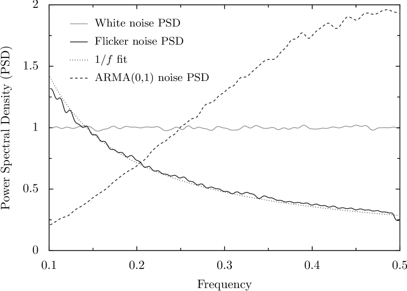
Figure 3.— Example of the structure that is expected in the power spectral density (PSD) of residual signals of the different types considered in this paper. The PSDs shown here are the mean of $10000$ realizations with the noise-structures indicated in the figure. Note that the white-noise PSD is flat, while the flicker-noise and the ARMA($0,1$) models cover low and high-frequency ranges. respectively.

In the past sub-sections we set up an estimation process for the signal given in eq. (2) using principal component analysis. It remains to specify a model for the stochastic signal which we have termed noise, i.e., the $\epsilon(t)$ term in eq. (1). As noted above, the principal components will absorb part of the $\epsilon(t)$, and so our estimate of the noise may not necessarily accurately reflect the $\epsilon(t)$ term in eq. (1) assuming the model holds. Nonetheless, this is of no consequence as we just aim to model the residuals after the time series has been modeled with the $\{s_{i}\}_{i=1}^{l}$. While we still call this term $\epsilon(t)$ in what follows, one should bear in mind this subtlety. An important feature of the correlated stochastic models we consider is that they can model trends. The $\{s_{i}\}_{i=1}^{l}$ are obtained from the comparison stars, and while the hope is that they capture all of the systematic effects, it is possible that some systematic effects individual to the target star are not captured. The stochastic “noise” models considered below that have time correlations can in principle capture remnant individual trends particular to WASP-6.

We make use of Markov Chain Monte Carlo (MCMC; see, e.g., Ford, 2005) algorithms to obtain estimates of the posterior probabilty distributions of our parameters, $\theta,\alpha,\eta$, given a dataset $\mathbf{y}$, where we have introduced a new set of parameters $\eta$ characterizing a stochastic component (see below). The posterior distribution $p(\mathbf{\theta,\alpha,\eta}|\mathbf{y})$ is obtained using a prior distribution for our parameters $p(\mathbf{\theta,\alpha,\eta})$ and a likelihood function, $p(\mathbf{y}|\mathbf{\theta,\alpha,\eta})$. Following previous works (e.g. Carter & Winn, 2009; Gibson et al., 2012) we assume that the likelihood function is a multivariate Gaussian distribution given by

$$p(\mathbf{y}|\mathbf{\theta,\alpha,\eta}) = \frac{1}{(2\pi)^{n/2}|\mathbf{\Sigma_{\eta}}|^{1/2}}$$

$$\times\exp\left[{-\frac{1}{2}(\mathbf{y}-\mathbf{g}(\theta,\alpha))^{T}\mathbf{\Sigma_{\eta}}^{-1}(\mathbf{y}-\mathbf{g}(\theta,\alpha))}\right],$$

where $\mathbf{g}(\theta,\alpha)$ is the function that predicts the observed datapoints and $\mathbf{\Sigma}_{\eta}$ is the covariance matrix which depends on the set of parameters $\eta$. It is the structure of this matrix which defines the type of noise of the residuals. Previous works have proposed to account for time correlated structure in the residuals using flicker noise models, where it is assumed that the noise follows a Power Spectral Density (PSD) of the form $1/f$ (Carter & Winn, 2009), and Gaussian processes, where the covariance matrix is parametrized with a particular kernel that can incorporate correlations depending on a set of input parameters, including time (Gibson et al., 2012, 2013) . In the present work we consider three different models: a white-noise model, where the covariance matrix is assumed to be diagonal, a flicker-noise model, and ARMA$(p,q)$ models, where the structure of the covariance is determined via the parameters $p$ and $q$ (see §4.2.2 below for the definition of ARMA$(p,q)$ models). The reason for choosing these three models is that they sample a wide range of spectral structure of the noise: white-noise models define models where the PSD is flat, while flicker and ARMA-like models define noise structures with PSDs with power in low and high frequencies, respectively. Figure 3 illustrates the various structures the PSD can have for the different noise structures considered here.

4.2.1 Flicker noise model

Flicker-noise is known to arise in many astrophysical time series (Press, 1978). It is a type of noise that fits long-range correlations in a stochastic process very well because of its assumed PSD shape of $1/f$. An efficient set of algorithms for its implementation in MCMC algorithms was proposed recently by Carter & Winn (2009). The basic idea of this implementation is to assume that the noise is made up of two components: an uncorrelated Gaussian process of constant variance and a correlated Gaussian process which follows this flicker-noise model. These two components are parametrized by $\sigma_{w}$ and $\sigma_{r}$, characterizing the white and correlated noise components, respectively. A wavelet transform of the residuals takes the problem into the wavelet basis where flicker noise is nearly-uncorrelated making the problem analytically and computationally more tractable.

4.2.2 ARMA noise model

Autoregressive-moving-average (ARMA) models have been in use in the statistical literature for a long time with a very broad range of different applications (Brockwell & Davis, 1991). Although known for long in the astronomical community (e.g., Scargle, 1981; Koen & Lombard, 1993), these noise models haven’t been used so far for transit lightcurves to the best of our knowledge.

The time series $X_{t_{k}}$ of an ARMA($p,q$) process, where the $t_{k}$ are the times of each observation, satisfies

$$X_{t_{k}}=\sum_{i=1}^{p}\phi_{i}X_{t_{k-i}}+\sum_{i=1}^{q}\theta_{i}\varepsilon(t_{k-i})+\varepsilon(t_{k}).$$ (5)

where the $\{\phi_{i}\}^{p}_{i=1}$ and $\{\theta_{i}\}^{q}_{i=1}$ are the parameters of the model and $\varepsilon_{t_{k}}$ is white noise with variance $\sigma_{w}^{2}$. The orders $(p,q)$ of the ARMA($p,q$) model define how far in the past a given process looks at when defining future values. Long-range correlations need a high order ARMA model, while short-range correlations need lower order models. An ARMA model allows us to explore a higher range of noise structures in a complementary way to flicker noise models.

In order to fit ARMA models to the residuals via an MCMC algorithm, we need the likelihood function of the model given that the residuals follow an ARMA($p,q$) model. For this we implented the recursive algorithm described in Brockwell & Davis (1991, Chapter 8), which assumes that $\varepsilon(t_{k})$ follows a normal distribution with constant variance and that the ARMA process is causal and invertible.

4.2.3 Stochastic model selection

Given the three proposed noise models for the stochastic signal $\epsilon(t)$, it remains to define which of the three affords a better description of the data, taking into account the trade-off between the complexity of the proposed model and its goodness-of-fit. There are several criteria for model selection, a comprehensive comparison between different criteria has been done recently by Vehtari & Ojanen (2012). The main conclusion is that, despite the fact that many model selection criteria have good asymptotic behavior under the constraints that are explicit when deriving them, there is no “perfect model selection” criteria, and there is a need to compare the different methods in the finite-sample case. Following this philosophy, we compare in this work the results of the AIC (“An Information Criterion”; Akaike, 1974), the BIC (“Bayesian Information Criterion”; Schwarz, 1978), the DIC (“Deviance Information Criterion”; Spiegelhalter et al., 2002) and the DIC^A, a modified version of DIC with a proposal for bias-correction (Ando, 2012).

5. Lightcurve analysis

From the initial ten comparison stars, only seven were used to correct for systematic effects. One star was eliminated on the grounds of having significantly less flux than the rest and the other two due to not having the whole spectral range of interest recorded in the CCD. Given the seven comparison stars, we applied PCA to the mean-substracted time-series in order to obtain an estimate of the perturbation signals. We describe now the construction and analysis of the white light transit light curve and the light curves for 20 wavelength bins.

5.1. White light transit light curve

In order to obtain the white light transit light curve of WASP-6, we summed the signal over the wavelength range $4718$ to $8879$ Å for the target and the comparison stars. Then, we performed $5$-fold cross-validation in the out-of-transit part of the light curve of WASP-6 in order to obtain the optimal number of components to be used in our MCMC algorithm. The result of this cross-validation procedure is shown in Figure 4.

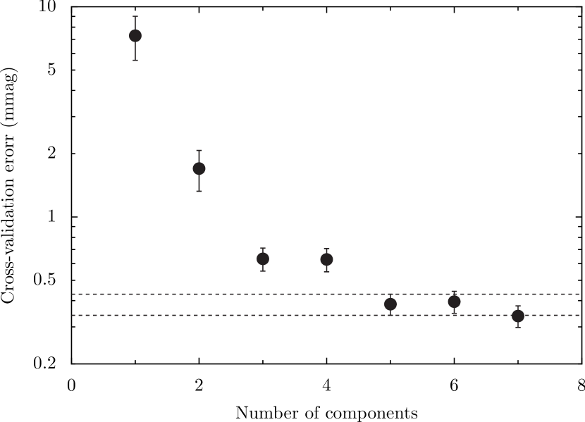
Figure 4.— Cross-validation error for the prediction of out-of-transit data using different number of principal components with the $5$-fold cross-validation procedure we adopted. Note that the minimum is at $k=7$ (dashed lines indicate the value at the minimum and a value higher by $1\sigma$), but the value at $k=5$ achieves similar error with lower degrees of freedom.

From the results of our $5$-fold cross-validation procedure one may choose either $k=7$ (the value of the minimum error) or $k=5$, which is at less than 1-standard error away from the value at the minimum. We choose this last value because it allows a similar prediction error as the minimum with two less parameter.

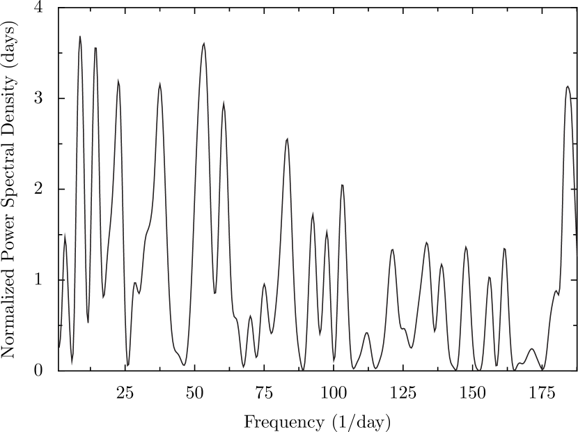
Figure 5.— Power spectral density of the residuals of the fit using white Gaussian noise (see Figure 6 to see the residuals). Note the preference for high power at small frequencies.

Using the first five principal components, we fitted the model proposed in Equation 1 first using a white Gaussian noise model via MCMC using the PyMC python module (Patil et al., 2010). We used wide truncated Gaussian priors in order to incorporate previous measurements of the transit parameters obtained by Gillon et al. (2009) and Dragomir et al. (2011), and the orbital parameters of Gillon et al. (2009). We adopt a quadratic limb darkening law of the form $I(\mu)=I(1)[1-u_{1}(1-\mu)-u_{2}(1-\mu)^{2}]$, where $\mu=\cos(\theta)$ and $\{u_{1},u_{2}\}$ are the limb darkening coefficients. It is well known that $u_{1}$ and $u_{2}$ are strongly correlated (Pál, 2008), and it has been shown that if we define new coefficients $(w_{1},w_{2})$ that are related to $(u_{1},u_{2})$ by $(w_{1},w_{2})=R(\pi/4)(u_{1},u_{2})$ where

$$R(\theta)=\left(\begin{array}[]{cc}\cos(\theta)&-\sin(\theta)\\ \sin(\theta)&\cos(\theta)\\ \end{array}\right)$$

is a rotation matrix by $\theta$ radians, then $w_{1},w_{2}$ are nearly uncorrelated and transits are mostly sensitive to $w_{1}$, with $w_{2}$ essentially constant (Howarth, 2011). In our MCMC analysis we fix $w_{2}$ to the (wavelength dependent) value calculated for the stellar parameters of WASP-6 as described in Sing (2010).

Five MCMC chains of $10^{6}$ links each, plus $10^{5}$ used for burn-in, where used. We checked that every chain converged to similar values and then thinned the MCMC samples by $10^{4}$ in order to get rid of the auto-correlation between the links. We used the thinned sample as our posterior distribution, using the posterior median as an estimate of each parameter (using the point in the chain with the largest likelihood leads to statistically indistinguishable results). The fit using a white Gaussian model for the noise allows us to investigate the structure of the residuals, which show clear long-range correlations, as is evident in the power spectral density of the residuals plotted in Figure 5. Note that the power is significantly higher at lower frequencies, which suggest that the residuals have long-range correlations. We performed an MCMC fit using an $1/f$-like and another MCMC fit using an ARMA-like model for the residuals. Note that in order to fit an ARMA($p$,$q$) model with our algorithms, we need to define the order $p$ and $q$ of the ARMA process. In order to do this, we fitted several ARMA($p$,$q$) models to the residuals of the white Gaussian MCMC fit for different orders $p$ and $q$ using maximum likelihood, and calculated the AIC and BIC of each fit. In the sense of minimizing these information criteria, the “best” ARMA model was an ARMA($2$,$2$) model, so we performed our MCMC algorithms assuming this as the best model for the ARMA case. The results of the MCMC fits assuming a white Gaussian noise model, an ARMA(2,2) noise model and a $1/f$ noise model for the residuals are shown in Figure 6, and a summary of the values of the information-criteria for each of our MCMC fits are shown in Table 2.

Table 2Values for the different information criteria (IC) for each noise-model considered in our MCMC fits.

IC	WG model${}^{\textrm{a}}$	ARMA$(2,2)$ model${}^{\textrm{a}}$	$1/f$ model${}^{\textrm{a}}$
AIC	-1260.59	-1273.38	-1833.72
BIC	-1230.46	-1234.20	-1801.08
DIC	-1165	-1202.03	-1793.60
DIC${}^{\textrm{A}}$	-1105.20	-1149.86	-1760.53

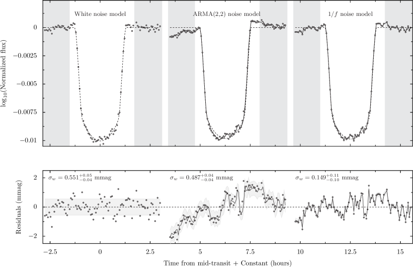
Figure 6.— (Top) The circles show the baseline-substracted lightcurves (i.e., lightcurves with the fitted perturbation signal substracted) using the different noise models indicated. We also show the corresponding best-fit transit models (dashed line) and the best-fit transit models plus an estimate of the correlated noise component (solid line, only for the two right-most lightcurves). The shaded regions indicate points that where used as out-of-transit data by the $5$-fold cross-validation procedure that selected the number of principal components to use in the fits. (Bottom) Residuals between the best-fit transit model and the baseline subtracted lightcurves (circles). The solid lines in the two right-most set of points indicate estimates of the correlated components obtained by projecting the residuals into the best-fit correlated component model (see §5). The difference between the points and the solid lines (dashed line for the white Gaussian noise case) is the white Gaussian noise component, whose dispersion $\sigma_{w}$ is indicated for each of the noise models considered and also illustrated with $\pm 1\sigma_{w}$ bands.

Table 3MCMC priors used for the white light transit analysis.

Transit parameter	Description	Prior${}^{\textrm{a}}$	Units
$R_{p}/R_{s}$	Planet-to-star radius ratio	TruncNorm$(0.14,0.01^{2})^{A}$	-
$t_{0}$	Time of mid-transit	TruncNorm$(55473.15,0.01^{2})^{c}$	MHJD
$P$	Period	TruncNorm$(3.36,0.01^{2})^{b}$	days
$i$	Inclination	TruncNorm$(1.546,0.017^{2})^{b}$	Radians
$R_{s}/a$	Stellar radius to semi-major axis ratio	TruncNorm$(0.09,0.01^{2})^{b}$	-
$w_{1}$	Linear limb-darkening coefficient	U$(0,1)$	-
$\sigma_{w}$	Standard deviation of the white noise part of the noise model	U$(0,1)$	mag
$\sigma_{r}$	Noise parameter for the $1/f$ part of the noise model${}^{\textrm{d}}$	U$(0,1)$	mag

Table 4WASP-6b transit parameters estimated using the white light transit lightcurve using a $1/f$-like noise model.

Transit parameter	Description	Posterior value	Units
$R_{p}/R_{s}$	Planet-to-star radius ratio	$0.1404^{+0.0010}_{-0.0010}$	-
$t_{0}$	Time of mid-transit	$55473.15365^{+0.00016}_{-0.00016}$	MHJD
$P$	Period	$3.3605^{+0.0098}_{-0.0101}$	days
$i$	Inclination	$1.5465^{+0.0074}_{-0.0055}$	Radians
$R_{s}/a$	Stellar radius to semi-major axis ratio	$0.0932^{+0.0015}_{-0.0015}$	-
$w_{1}$	limb-darkening coefficient (see § 5.1)	$0.44^{+0.12}_{-0.12}$	-
$\sigma_{w}$	Standard deviation of the white noise part of the noise model	$0.1492^{+0.1078}_{-0.1021}$	mmag
$\sigma_{r}$	Noise parameter for the $1/f$ part of the noise model${}^{\textrm{a}}$	$3.26^{+0.03}_{-0.50}$	mmag

It is important to note that the residuals shown in Figure 6 are the signal left over after subtracting the deterministic part of the model only (denoted by $\mathbf{g}(\theta,\alpha)$ in equation 4.2). Therefore, they still contain in the case of the ARMA(2,2) and $1/f$ noise models, a correlated stochastic component summed with a white noise component. As opposed to deterministic components, the stochastic components cannot just be predicted given the times $t_{i}$ of the observations, as we only know the distribution of expected values once we know the parameters ($\{\theta_{1},\theta_{2},\phi_{1},\phi_{2},\sigma_{w}\}$ for ARMA(2,2), $\{\sigma_{r},\sigma_{w}\}$ for flicker noise and $\sigma_{w}$ for white Gaussian noise). But even though we cannot plot a unique expected trend given the best-fit parameters for the correlated noise models, we can apply filters to the residuals that project them into the best-fit model, or viewed differently, we can filter out the expected white Gaussian noise component leaving just the correlated part. Such filters allow us then to build estimates of the particular realization of a given process that is present in our residuals. For the ARMA(2,2) and $1/f$ case we plot in the bottom panel of Figure 6 estimates of the correlated components as solid lines through the residuals. It is the difference between these lines and the residual points that constitute the remaining white Gaussian noise component with dispersion $\sigma_{w}$ indicated in the residuals panel.

It is informative to discuss the different values of the $\sigma_{w}$ parameter inferred for each of the models we consider. For the white Gaussian noise model, the value of this parameter is $\sigma_{w}=0.55^{+0.05}_{-0.04}$ mmag, which is an order of magnitude higher than the underlying Poisson noise ($\approx$ 0.06 mmag, see § 2). The same goes for the ARMA-like noise model fit, which has a value of this parameter of $\sigma_{w}=0.49^{+0.04}_{-0.04}$ mmag. Finally, for the $1/f$-like noise model the value of this parameter is $\sigma_{w}=0.15^{+0.11}_{-0.10}$ mmag, which is just $\approx 2.5$ times the Poisson noise limit. Motivated by this result and by the values of the information-theoretic model selection measures quoted on Table 2, we conclude that the preferred model is the one that models the underlying stochastic signal as $1/f$-like noise. We note that as Carter & Winn (2009) stress in their work, using this model for the residuals increases the uncertainty in the transit parameter, but provides more realistic estimates for them. We select the model parameters fitted using the $1/f$ noise model, which are quoted in Table 4, as the best estimates from now on. These parameters are generally an improvement on previous measurements by Gillon et al. (2009) and Dragomir et al. (2011).

We close this section by noting that the principal component regression we adopted was able to recover from the high periods of absorption present 0–2 hrs after mid-transit (see Figure 2) without leaving a noticeable trace in the final light curve.

5.2. WASP-6b transmission spectrum

The procedures explained in the previous sub-section were replicated for the time series of each of 20 wavelength bins, but now leaving only the planet-to-star radius ratio, the linear limb darkening coefficient $w_{1}$ and the noise parameters as free parameters (all the other transit parameters where fixed to the values shown in Table 4 while the values for $w_{2}$ are calculated as indicated in § 5.1 and are indicated in Table A Ground-based Optical Transmission Spectrum of WASP-6b). Priors were the same as the white light analysis for parameters for $\mu_{1},\sigma_{r}$ and $\sigma_{w}$, and the MCMC chains were set-up similarly except that a thinning value of $10^{3}$ was used. The prior for $(R_{pl}/R_{*})$ was set to $TruncNorm(0.1404,0.01^{2})$, i.e. we set the mean to the posterior value of our white light analysis. The wavelength bins were chosen to be $\approx$ 200 Å wide, with boundaries that lie in the pseudo-continuum of the WASP-6 spectrum, as boundaries in steep parts of the spectrum such as spectral lines would in principle maximize redistribution of flux between adjacent bins under the changing seeing conditions which set the spectral resolution in our setup. For a given spectral bin, the number of principal components was selected separately because different systematics may be dependent on wavelength, and therefore the number of principal components needed may change. In practice, no more than one principal component was added or subtracted in each wavelength bin when compared to the five components used for the white light curve. In all of them, however, the noise model to be used is the same, the $1/f$-like noise model. Figure 7 shows the baseline-substracted data along with the best-fit transit model at different wavelengths, and Table A Ground-based Optical Transmission Spectrum of WASP-6b tabulates the transit parameters from the MCMC analysis for each wavelength bin. The values of $R_{\rm pl}/R_{*}$ as a function of wavelength constitute our measured transmission spectrum which is shown in Figure 8; the typical uncertainty in $R_{\rm pl}/R_{*}$ is $\approx 0.8$%, and the inferred $\sigma_{w}$ values are typically $\approx$ 1–3 times the Poisson limit in each wavelength bin, for which a typical value is 0.25 mmag.

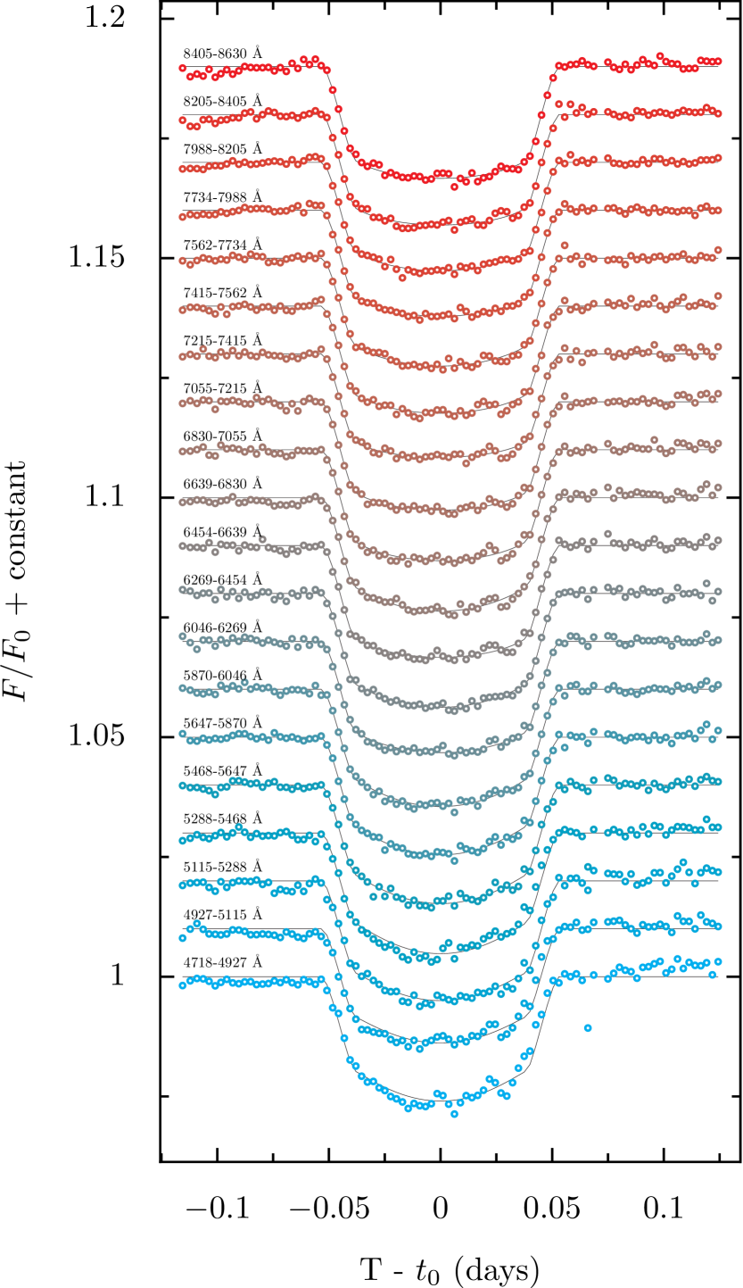
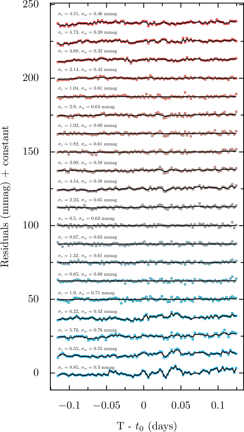
Figure 7.— (Left) Transits as observed in different wavelength channels along with the best-fit transit signal plus the stochastic $1/f$ noise signal. The obvious outlier close to $t-t_{0}=0.05$ at the first, bluest, wavelength bin was not included in the fit. (Right) Residuals between the best-fit transit model and the baseline subtracted lightcurves for each of the wavelength channels (circles). The solid lines indicate estimates of the correlated $1/f$ component obtained as described in §5. The best fit parameters of the $1/f$ component are indicated over each set of residuals.

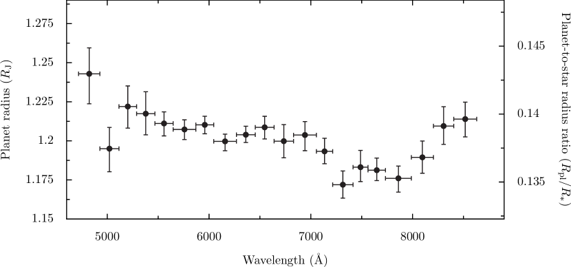
Figure 8.— Transmission spectrum of WASP-6b measured with IMACS.

5.3. Limits on the contribution of unocculted stellar spots

As pointed out in several works (e.g., Pont et al., 2008; Sing et al., 2011b), stellar spots – both occulted and unocculted during transit – can affect the transmission spectrum. In our transit light curve we see no significant deviations that could be attributed to an occulted starspot, so in what follows we estimate the potential signal induced in the transmission spectrum by unocculted stellar spots.

Stellar spots can be modelled as regions in the surface of the star that have a lower effective temperature that the photosphere. Given that WASP-6 is a G star, we can use the Sun as a proxy to infer spot properties. Sunspots can be characterized as having a temperature difference with the photosphere of $\Delta T\approx-500$ K (Lagrange et al., 2010, see §2.2). This is an effective value that represents a good average for the different values of $\Delta T$ in the umbral and penumbral regions. Given a fraction of the stellar surface $f_{s}$ covered by spots characterized by temperature $T+\Delta T$, the total brightness of the star will be changed by a factor $1+f(\lambda)=1+f_{s}(I_{\lambda}(T+\Delta T,\theta)/I_{\lambda}(T,\theta)-1)$, where $I_{\lambda}(T,\theta)$ is the surface brightness of a star with effective temperature $T$ and other stellar parameters given by $\theta=(\log g,Z,\ldots)$. If the fractional change in flux $\epsilon$ caused by spots at a reference wavelength $\lambda_{0}$ can be measured then $f_{s}$ can be inferred to be $f_{s}=\epsilon/(I_{\lambda_{0}}(T+\Delta T,\theta)/I_{\lambda_{0}}(T,\theta)-1)$ and then we can write $f(\lambda)=\epsilon(I_{\lambda}(T+\Delta T,\theta)/I_{\lambda}(T,\theta)-1)(I_{\lambda_{0}}(T+\Delta T,\theta)/I_{\lambda_{0}}(T,\theta)-1)^{-1}$ (c.f. Sing et al., 2011b, eq. 4).

A change in the stellar luminosity due to starspots will have an effect on the measured value of $k=R_{p}/R_{*}$, and as the effect is chromatic, it will induce an effect in the tranmission spectrum. The decrease of flux during transit with respect to the out of transit flux $F_{0}$ is given by $(\Delta F/F_{0})=k^{2}$ (neglecting any emission from the planet). If $F_{0}$ is changed by starspots by a fractional amount $f(\lambda)$ we have $\delta(\Delta F/F_{0})\approx-(\Delta F/F_{0})\delta F_{0}/F_{0}\equiv-(\Delta F/F_{0})f(\lambda)=k^{2}f(\lambda)=2k\delta k$, where we have used $f(\lambda)\equiv\delta F_{0}/F_{0}$. From here we get finally

$$\frac{\delta k}{k}=\frac{-f(\lambda)}{2}.$$

We used the method described in Maxted et al. (2011) to look for periodic variations due to spots in the lightcurves of WASP-6 from the WASP archive (Pollacco et al., 2006). Data from 3 observing seasons were analysed independently. The lightcurves typically contain $\sim$4500 observations with a baseline of 200 nights. From the projected equatorial rotation velocity of WASP-6 and its radius (Doyle et al., 2013) we estimate that the rotation period is $16\pm 3$  days. There are no significant periodic variations in this range in any of the WASP lightcurves. To estimate the false alarm probability of any peaks in the periodogram we use a bootstrap Monte Carlo method. The results of this anaysis can also be used to estimate an upper limit of 2 mmag to the amplitude of any periodic variation in these lightcurves. Therefore, $\epsilon$ is constrained to be less than the implied peak-to-peak amplitude, $|\epsilon|<4$ mmag. While this constraint is valid only at the time the discovery light curve was taken, lacking any other constrains we will take this value as our upper limit. In order to estimate $f(\lambda)$ we make use of the high resolution Phoenix synthetic stellar spectra computed by Husser et al. (2013). We assume $T=5400$ K, $\Delta T=-500$ K, and other stellar parameters to be the closest available in the models grid to those presented in Gillon et al. (2009). The resulting expected maximum value for $\delta k/k$ given the constrains on the rotational modulation afforded by the WASP-6 discovery light curve is presented in Figure 9. As can be seen, the change in $\delta k/k$ induced by starspots over the wavelength range of our spectrum is expected to be $<5\times 10^{-4}$. This is more than one order of magnitude less than the change we in $\delta k/k$ we infer from our observations (see Figure 8), and thus we conclude that the observed transmission spectrum is not produced by unocculted spots.

Figure 9.— Predicted fractional change in $k=(R_{p}/R_{*})$ due to stellar spots that produce a rotation amplitude of $\epsilon=-4$ mmag in the $V$ band. The spots are assumed to have a temperature lower than that of the photosphere by $\Delta T=-500$ K.

6. The Transmission Spectrum: Analysis

The main feature of the transmission spectrum shown in Figure 8 is a general sloping trend with $R_{p}/R_{*}$ becoming smaller for longer wavelengths. The general trend is broken by the two redmost datapoints that could be indicating the presence of a source of opacity in that region, but the error bars of the extreme points are large, as the measurements there are naturally more uncertain because the spectrograph efficiency changes drops rapidly at the red end of the spectrum and this region of the spectrum can be badly affected by variations in night sky emission and telluric absorption. There are no indications of the broad features expected at the resonance doublets of Na I at 589.4 nm or K I at 767 nm. To make the statements above quantitative, we compare our measured transmission spectrum with the clear atmosphere models computed by Fortney et al. (2010). We scale the models that have a surface gravity of $g=10$ m/s² to match the measured surface gravity of WASP-6b ($g=8.71$ m/s², Gillon et al., 2009) by scaling the spectral features from the base level by $10/g$. We do not have an absolute reference to be able to place the 10 bar level such as could be provided by observations at infra-red wavelengths, which in the Fortney et al. (2010) models is set to 1.25 $R_{J}$, and so we fit for an overall offset in the $y$-axis. In other words, our measured transmission spectrum will be able to discriminate on the shape of the models but will provide no independent information on the absolute height in the atmosphere where the features are formed. Given that the equilibrium planet temperature assuming no albedo and full redistribution between the day and night sides is $T_{\rm eff}=1194^{+58}_{-57}$ K (Gillon et al., 2009) we will compare our measurements with the $T=1000$ and $T=1500$ K models of Fortney et al. (2010). The $T=1000$ K model has Na and K as the main absorbers, while the $T=1500$ K model also displays the effects of partially condensed TiO and VO resulting in a very different transmission spectra.

In addition to clear atmosphere models we fit our data to a pure scattering spectrum as given by Lecavelier Des Etangs et al. (2008) for a scattering cross section $\sigma=\sigma_{0}(\lambda/\lambda_{0})^{\alpha}$,

$$\frac{d\,R_{p}}{d\,\ln\lambda}=\alpha H_{c}=\frac{\alpha k_{B}T}{\mu g},$$ (6)

where $H_{c}$ is the scale-height of the particles producing the scattering, which we assume to be equal to the gaseous scale height $H=k_{B}T/\mu g$, although condensates producing scattering can have smaller scale heights than the gas, $H_{c}\sim H/3$, unless they are very well mixed vertically (Fortney, 2005). In the case of pure scattering we will fit for two parameters to match to our observed spectrum, the combination $\xi=\alpha T$, and a zero-point offset. We can then interpret the value of $\xi$ assuming Rayleigh scattering $\alpha=-4$ or the expected values of the equlibrium temperature for the atmosphere of WASP-6b.

Along with the transmission spectrum, Figure 10 shows the results of fitting the models to our observed transmission spectrum. It is clear to the eye that the best fit is given by the pure scattering model, with the clear atmosphere models giving considerably worse fits. The clear atmosphere models fail to give a better match to the spectrum due to the lack in the latter of evidence for the broad features expected around Na and K. The AIC for the scattering model assuming Gaussian noise given by the known error bars gives $-115.3$, while the values for the $T=1000$ and $T=1500$ clear atmosphere models are $-97.2$ and $-90.9$ respectively, providing a very significant preference for the scattering model. A $\chi^{2}$ analysis gives a $p$-value of 0.04 for the pure scattering model ($\chi^{2}=30$ for 18 degrees of freedom), while the probabilities for the data being produced by either of the clear atmosphere models are exceedingly small ($\chi^{2}=80$ and $106$ with 19 degrees of freedom for the $T=1000$ and 1500 models, respectively, giving $p$-values $<10^{-8}$ for both). Based on the numbers above, only the scattering model is viable, but these analyses ignore potential correlation of the errors in the wavelength dimension. Looking at the light curves in Figure 7 one can see that in some cases features in the light curves repeat between adjacent wavelength channels. In order to assess the potential impact of correlations in the wavelength direction, we compute the partial autocorrelation function (PACF) for the residuals in the wavelength dimension. Denoting the residuals of the transit fits shown in Figure 7 by $r_{il}$, where $i$ indexes time and $l$ the wavelength channel, we compute the PACF for the 20 vectors $(r_{1l},r_{2l},\ldots,r_{nl})$ with $l=1,\ldots,20$ and $n=91$. The PACF has one significant component at lag 1, which shows that the residuals have indeed correlations with the adjacent channels that are suggestive of an AR(1) correlation struture. This does not imply that the $(R_{p}/R_{*})_{\lambda}$ values will necessarily have such correlation, but we should check how the models fare when including such potential correlation structure in the fits.

We performed fits then of all three models including an AR(1) component, to see if it gave a significantly better model as gauged by the information criteria listed in § 4.2.3. The scattering model does not need an additional AR(1) component, while for the clear atmosphere models including correlation gives a significantly better fit. This should come as no surprise, as the clear atmosphere models give a poor fit to start with, and including an extra AR(1) component can effectively model some of the residual structure. But even after accounting for potential correlation structure on them, the scattering model is significantly better than clear atmosphere models. We conclude therefore that our measured transmission spectrum is most consistent with a featureless sloped spectrum and does not present significant evidence for the features predicted by clear atmosphere models even if trying to account for the differences between the model and the observations with correlated errors with short lags between the wavelength channels as suggested by the residuals in the light curves.

The best-fit value for $\xi$ is $\xi=-10670\pm 3015$. If we fix the temperature to the equilibrium value given by Gillon et al. (2009), then we would infer $\alpha=-9\pm 2.5$ and, inversely, when assuming Rayleigh scattering we’d infer a temperature of $T=2667\pm 750$ K. The inferred values for $\alpha$ and $T$ are consistent within 2$\sigma$ from the values for Rayleigh scattering and the equilibrium temperature $T=1194^{+58}_{-57}$ given by Gillon et al. (2009), but the uncertainties are too large to allow any further conclusions, especially when considering the additional uncertainty in the scale height assigned to the material responsible for the scattering.

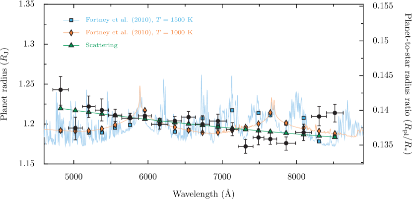
Figure 10.— Transmission spectrum of WASP-6b along with various models. Black dots with error bars indicate our measurements, while blue squares indicate the binned model of Fortney et al. (2010) with $T_{\rm{eq}}=1500$ K and red diamonds indicate the binned model using $T_{\rm{eq}}=1500$ K. The green-line and triangles indicate the best-fit line for a scattering model, which is the favored model in this case.

7. Discussion and Conclusions

We have measured the optical transmission spectrum for WASP-6b in the range $\approx$ 480 to 860 nm via differential spectrophotometry using 7 comparison stars with the IMACS spectrograph on Magellan. By modeling the systematic effects via a principal component analysis of the available comparison stars and a white-noise model for the noise, we are able to achieve light curve with residuals of order $\approx 0.8$ mmag in 200 nm channels per 140 sec exposure, and $\approx 0.5$ mmag in the summed (white-light) light curve. In order to take into account possible remaining trends particular to the target star and the correlated structure of the noise we probe the appropriateness of both short (ARMA(p,q)) and long ($1/f$ “flicker” noise) stochastic process, making use of well established information criteria to select the model most appropriate for our particular observations which turned out to be the $1/f$ model. We believe it is fundamental to carry out a residual analysis for each particular observation. Lacking a detailed physical model for a given correlation structure it should be the data that select which is the most appropriate for a given observation. With the $1/f$ model the inferred white noise components are $\approx$ 1–3 times the expected Poisson shot noise ($\sigma_{w}=0.16$ mmag per 140 sec exposure for the white light curve and $\sim 0.6$ mmag per 140 sec exposure for the 200nm channels).

The measured spectrum has a general trend of decreasing planetary size with wavelength, and does not display any evident additional features. We fit our transmission spectrum with three different models: two clear transmission spectra from Fortney et al. (2010) and a spectrum caused by pure scattering. Our main conclusion is that the transmission spectrum of WASP-6b is most consistent with that expected from a scattering process that is more efficient in the blue. In addition, the spectrum does not show the expected broad features due to alkali metals expected in clear atmosphere models which give significantly less satisfactory description of our data, even when allowing for the errors to be correlated between different wavelength bins.

We conclude that the spectrum is most consistent with a featureless spectrum that can be produced by scattering. The potentially prominent role of condensates or hazes in determining the transmission spectra of exoplanets has been apparent from the very first measurement (Charbonneau et al., 2002), and our transmission spectrum of WASP-6b is in line with what seems to be building trend for transmission spectra with muted features in the optical. Higher resolution observations around the alkali lines for WASP-6b will be valuable to see if they remain at detectable levels over the mechamism that is veiling the very broad lines that are expected for clear atmospheres. We note that the expected equilibrium temperature for WASP-6b is similar to that of HD 189733b, so it may be the case that a similar obscurer is acting in both systems.

Our work adds a new instrument (IMACS) to the rapidly increasing set of ground-based facilities that have been succesfully used to probe exoplanetary atmospheres. The constraints that can be obtained using ground-based facilities is a powerful complement to those possible from space-based facilities and allow us to access a much broader pool of systems more representative of the typical brightness of hosts discovered by ground-based transit surveys. An interesting goal enabled by this capability will be to probe the transmission spectra of gas giants with fairly similar surface gravities as a function of equilibrium temperatures.

Table 5Transit parameters as a function of wavelength

Wavelength range	$(R_{p}/R_{*})$	$w_{1}$	$w_{2}^{\textrm{a}}$	$\sigma_{w}$	$\sigma_{r}$	$\sigma_{\rm Poisson}^{\textrm{b}}$
Å				mmag	mmag	mmag
4718–4927	$0.1430^{+0.0019}_{-0.0022}$	$0.9303^{+0.0523}_{-0.1043}$	0.2047	$0.3048^{+0.2399}_{-0.2007}$	$8.8352^{+0.8051}_{-0.8850}$	0.31
4927–5115	$0.1375^{+0.0016}_{-0.0017}$	$0.8705^{+0.0935}_{-0.1616}$	0.2016	$0.5409^{+0.2104}_{-0.2841}$	$6.5492^{+1.3376}_{-1.6895}$	0.29
5115–5288	$0.1406^{+0.0015}_{-0.0016}$	$0.9127^{+0.0621}_{-0.1148}$	0.1955	$0.7520^{+0.2008}_{-0.2591}$	$5.8071^{+1.9512}_{-2.0652}$	0.30
5288–5468	$0.1400^{+0.0016}_{-0.0016}$	$0.9430^{+0.0427}_{-0.0793}$	0.2254	$0.4151^{+0.1765}_{-0.2394}$	$6.3147^{+0.9081}_{-1.1713}$	0.27
5468–5647	$0.1393^{+0.0009}_{-0.0009}$	$0.8508^{+0.0912}_{-0.1080}$	0.2326	$0.7546^{+0.0771}_{-0.1372}$	$1.8322^{+2.0657}_{-1.3047}$	0.26
5647–5870	$0.1389^{+0.0007}_{-0.0007}$	$0.8114^{+0.0812}_{-0.0824}$	0.2429	$0.6957^{+0.0492}_{-0.0465}$	$0.6417^{+0.7686}_{-0.4527}$	0.23
5870–6046	$0.1392^{+0.0006}_{-0.0007}$	$0.7259^{+0.0866}_{-0.0897}$	0.2467	$0.6109^{+0.0550}_{-0.0688}$	$1.3599^{+1.1107}_{-0.9551}$	0.25
6046–6269	$0.1380^{+0.0005}_{-0.0007}$	$0.4206^{+0.0897}_{-0.0831}$	0.2477	$0.6289^{+0.0512}_{-0.0456}$	$0.6554^{+0.8881}_{-0.4690}$	0.22
6269–6454	$0.1385^{+0.0006}_{-0.0006}$	$0.5400^{+0.0801}_{-0.0827}$	0.2515	$0.6345^{+0.0452}_{-0.0441}$	$0.4624^{+0.6751}_{-0.3109}$	0.24
6454–6639	$0.1390^{+0.0008}_{-0.0009}$	$0.2265^{+0.1195}_{-0.1152}$	0.2718	$0.6525^{+0.0807}_{-0.1469}$	$2.2304^{+1.7794}_{-1.6389}$	0.24
6639–6830	$0.1380^{+0.0012}_{-0.0012}$	$0.5771^{+0.1581}_{-0.1621}$	0.2526	$0.4817^{+0.1580}_{-0.2070}$	$4.5171^{+1.2569}_{-1.5051}$	0.23
6830–7055	$0.1385^{+0.0010}_{-0.0012}$	$0.3163^{+0.1538}_{-0.1399}$	0.2500	$0.5873^{+0.1152}_{-0.2005}$	$2.9911^{+1.8578}_{-1.9120}$	0.22
7055–7215	$0.1373^{+0.0010}_{-0.0009}$	$0.2642^{+0.1219}_{-0.1172}$	0.2484	$0.6105^{+0.0675}_{-0.0939}$	$1.8425^{+1.3572}_{-1.1820}$	0.27
7215–7415	$0.1348^{+0.0010}_{-0.0010}$	$0.1628^{+0.1236}_{-0.0973}$	0.2481	$0.6886^{+0.0561}_{-0.0648}$	$1.0756^{+1.2399}_{-0.7853}$	0.25
7415–7562	$0.1361^{+0.0012}_{-0.0011}$	$0.3190^{+0.1354}_{-0.1297}$	0.2492	$0.6276^{+0.0957}_{-0.1215}$	$2.9063^{+1.2681}_{-1.5044}$	0.30
7562–7734	$0.1359^{+0.0009}_{-0.0008}$	$0.4066^{+0.1013}_{-0.0971}$	0.2493	$0.6145^{+0.0506}_{-0.0603}$	$1.0299^{+1.1571}_{-0.7499}$	0.31
7734–7988	$0.1353^{+0.0009}_{-0.0010}$	$0.3353^{+0.1135}_{-0.1066}$	0.2494	$0.4310^{+0.0654}_{-0.0670}$	$2.1595^{+0.7171}_{-0.7261}$	0.24
7988–8205	$0.1368^{+0.0012}_{-0.0012}$	$0.3408^{+0.1393}_{-0.1434}$	0.2478	$0.3215^{+0.0903}_{-0.1173}$	$3.6847^{+0.6986}_{-0.6914}$	0.28
8205–8405	$0.1391^{+0.0014}_{-0.0013}$	$0.2065^{+0.1626}_{-0.1316}$	0.2471	$0.3888^{+0.1214}_{-0.1655}$	$4.7549^{+0.8495}_{-0.9059}$	0.31
8405–8630	$0.1396^{+0.0012}_{-0.0013}$	$0.2599^{+0.1584}_{-0.1405}$	0.2454	$0.4683^{+0.0991}_{-0.1517}$	$4.4703^{+0.9456}_{-0.8350}$	0.30

References

- Akaike (1974) Akaike, H. 1974, IEEE Transactions on Automatic Control, 19, 716
- Alonso et al. (2004) Alonso, R., Brown, T. M., Torres, G., et al. 2004, ApJ, 613, L153
- Ando (2012) Ando, T. 2012, American Journal of Mathematical and Management Sciences, 31, 13
- Bakos et al. (2004) Bakos, G., Noyes, R. W., Kovács, G., et al. 2004, PASP, 116, 266
- Bakos et al. (2013) Bakos, G. Á., Csubry, Z., Penev, K., et al. 2013, PASP, 125, 154
- Bean et al. (2013) Bean, J. L., Désert, J.-M., Seifahrt, A., et al. 2013, ApJ, 771, 108
- Bean et al. (2011) Bean, J. L., Désert, J.-M., Kabath, P., et al. 2011, ApJ, 743, 92
- Borucki et al. (2010) Borucki, W. J., Koch, D., Basri, G., et al. 2010, Science, 327, 977
- Brockwell & Davis (1991) Brockwell, P., & Davis, R. 1991, Time Series: Theory and Methods, 2nd edn., Springer Series in Statistics (Springer Verlag)
- Brown (2001) Brown, T. M. 2001, ApJ, 553, 1006
- Carter & Winn (2009) Carter, J. A., & Winn, J. N. 2009, ApJ, 704, 51
- Charbonneau et al. (2002) Charbonneau, D., Brown, T. M., Noyes, R. W., & Gilliland, R. L. 2002, ApJ, 568, 377
- Colón et al. (2012) Colón, K. D., Ford, E. B., Redfield, S., et al. 2012, MNRAS, 419, 2233
- Deming et al. (2013) Deming, D., Wilkins, A., McCullough, P., et al. 2013, arXiv:1302.1141
- Désert et al. (2011) Désert, J.-M., Sing, D., Vidal-Madjar, A., et al. 2011, A&A, 526, A12
- Doyle et al. (2013) Doyle, A. P., Smalley, B., Maxted, P. F. L., et al. 2013, MNRAS, 428, 3164
- Dragomir et al. (2011) Dragomir, D., Kane, S. R., Pilyavsky, G., et al. 2011, AJ, 142, 115
- Dressler et al. (2011) Dressler, A., Bigelow, B., Hare, T., et al. 2011, PASP, 123, 288
- Ford (2005) Ford, E. B. 2005, AJ, 129, 1706
- Fortney (2005) Fortney, J. J. 2005, MNRAS, 364, 649
- Fortney et al. (2010) Fortney, J. J., Shabram, M., Showman, A. P., et al. 2010, ApJ, 709, 1396
- Gibson et al. (2013) Gibson, N. P., Aigrain, S., Barstow, J. K., et al. 2013, MNRAS, 428, 3680
- Gibson et al. (2012) Gibson, N. P., Aigrain, S., Roberts, S., et al. 2012, MNRAS, 419, 2683
- Gillon et al. (2009) Gillon, M., Anderson, D. R., Triaud, A. H. M. J., et al. 2009, A&A, 501, 785
- Hastie et al. (2007) Hastie, T., Tibshirani, R., & Friedman, J. 2007, Elements of Statistical Learning, 2nd edn., Springer Series in Statistics (Springer Verlag)
- Howarth (2011) Howarth, I. D. 2011, MNRAS, 418, 1165
- Husser et al. (2013) Husser, T.-O., Wende-von Berg, S., Dreizler, S., et al. 2013, A&A, 553, A6
- Jensen et al. (2012) Jensen, A. G., Redfield, S., Endl, M., et al. 2012, ApJ, 751, 86
- Koen & Lombard (1993) Koen, C., & Lombard, F. 1993, MNRAS, 263, 287
- Lagrange et al. (2010) Lagrange, A.-M., Desort, M., & Meunier, N. 2010, A&A, 512, A38
- Lecavelier Des Etangs et al. (2008) Lecavelier Des Etangs, A., Vidal-Madjar, A., Désert, J.-M., & Sing, D. 2008, A&A, 485, 865
- Lecavelier Des Etangs et al. (2010) Lecavelier Des Etangs, A., Ehrenreich, D., Vidal-Madjar, A., et al. 2010, A&A, 514, A72
- Mandel & Agol (2002) Mandel, K., & Agol, E. 2002, ApJ, 580, L171
- Marsh (1989) Marsh, T. R. 1989, PASP, 101, 1032
- Maxted et al. (2011) Maxted, P. F. L., Anderson, D. R., Collier Cameron, A., et al. 2011, PASP, 123, 547
- McCullough et al. (2005) McCullough, P. R., Stys, J. E., Valenti, J. A., et al. 2005, PASP, 117, 783
- Pál (2008) Pál, A. 2008, MNRAS, 390, 281
- Patil et al. (2010) Patil, A., Huard, D., & Fonnesbeck, C. J. 2010, Journal of Statistical Software, 35, 1
- Pepper et al. (2007) Pepper, J., Pogge, R. W., DePoy, D. L., et al. 2007, PASP, 119, 923
- Pollacco et al. (2006) Pollacco, D. L., Skillen, I., Collier Cameron, A., et al. 2006, PASP, 118, 1407
- Pont et al. (2008) Pont, F., Knutson, H., Gilliland, R. L., Moutou, C., & Charbonneau, D. 2008, MNRAS, 385, 109
- Pont et al. (2013) Pont, F., Sing, D. K., Gibson, N. P., et al. 2013, MNRAS, 432, 2917
- Press (1978) Press, W. H. 1978, Comments on Astrophysics, 7, 103
- Redfield et al. (2008) Redfield, S., Endl, M., Cochran, W. D., & Koesterke, L. 2008, ApJ, 673, L87
- Scargle (1981) Scargle, J. D. 1981, ApJS, 45, 1
- Schwarz (1978) Schwarz, G. 1978, Annals of Statistics, 6, 461
- Sing (2010) Sing, D. K. 2010, A&A, 510, A21
- Sing et al. (2008) Sing, D. K., Vidal-Madjar, A., Désert, J.-M., Lecavelier des Etangs, A., & Ballester, G. 2008, ApJ, 686, 658
- Sing et al. (2011a) Sing, D. K., Désert, J.-M., Fortney, J. J., et al. 2011a, A&A, 527, A73
- Sing et al. (2011b) Sing, D. K., Pont, F., Aigrain, S., et al. 2011b, MNRAS, 416, 1443
- Sing et al. (2012) Sing, D. K., Huitson, C. M., Lopez-Morales, M., et al. 2012, MNRAS, 426, 1663
- Snellen et al. (2008) Snellen, I. A. G., Albrecht, S., de Mooij, E. J. W., & Le Poole, R. S. 2008, A&A, 487, 357
- Spiegelhalter et al. (2002) Spiegelhalter, D., Best, N., Carlin, B., & van der Linde, A. 2002, Journal of the Royal Statistical Society, Series B, 64, 583
- Tuomi et al. (2013) Tuomi, M., Jones, H. R. A., Jenkins, J. S., et al. 2013, A&A, 551, A79
- Vehtari & Ojanen (2012) Vehtari, A., & Ojanen, J. 2012, Statistics Surveys, 6, 142
- Vidal-Madjar et al. (2003) Vidal-Madjar, A., Lecavelier des Etangs, A., Désert, J.-M., et al. 2003, Nature, 422, 143
- Vidal-Madjar et al. (2004) Vidal-Madjar, A., Désert, J.-M., Lecavelier des Etangs, A., et al. 2004, ApJ, 604, L69
- Wood et al. (2011) Wood, P. L., Maxted, P. F. L., Smalley, B., & Iro, N. 2011, MNRAS, 412, 2376
- Zhou & Bayliss (2012) Zhou, G., & Bayliss, D. D. R. 2012, MNRAS, 426, 2483