Isotope Spectroscopy

Abstract

The measurement of isotopic ratios provides a privileged insight both into nucleosynthesis and into the mechanisms operating in stellar envelopes, such as gravitational settling. In this article, we give a few examples of how isotopic ratios can be determined from high-resolution, high-quality stellar spectra. We consider examples of the lightest elements, H and He, for which the isotopic shifts are very large and easily measurable, and examples of heavier elements for which the determination of isotopic ratios is more difficult. The presence of ⁶Li in the stellar atmospheres causes a subtle extra depression in the red wing of the ⁷Li 670.7 nm doublet which can only be detected in spectra of the highest quality. But even with the best spectra, the derived ⁶Li abundance can only be as good as the synthetic spectra used for their interpretation. It is now known that 3D non-LTE modelling of the lithium spectral line profiles is necessary to account properly for the intrinsic line asymmetry, which is produced by convective flows in the atmospheres of cool stars, and can mimic the presence of ⁶Li. We also discuss briefly the case of the carbon isotopic ratio in metal-poor stars, and provide a new determination of the nickel isotopic ratios in the solar atmosphere.

1 Introduction

The knowledge of the chemical abundance pattern of a star gives us insights into the previous generations of massive stars that enriched the interstellar gas. The analysis of the isotopic ratios provides us with details about the different nuclear reactions involved and their relative contributions. These nuclear reactions could have taken place: (i) in the interiors of the previous generations of massive stars; (ii) during the final stages of stellar evolution in supernova explosions; (iii) in dynamical processes in late evolutionary phases of stars (s-process in AGB stars, mixing of CNO-processed material in RGB and AGB stars, hot-bottom burning, cool-bottom processing etc.); (iv) in the interstellar medium due to cosmic ray spallation events.

The analysis of isotopic ratios is considerably more difficult than the abundance determination, generally requiring extremely clean, high-quality spectra (highest spectral resolution and signal-to-noise ratio). Even then the isotopic ratio can be determined for only about 10% of the elements for which the photospheric abundance can be derived.

In the case that atomic lines are used in the isotopic analysis, the lighter the element the larger the wavelength shift between the lines of the different isotopes: for light elements, the isotopic shift is mainly due to the different masses of the isotopes, $m$ and $m^{\prime}$, such that $\Delta\lambda/\lambda^{2}\sim 1/m-1/m^{\prime}$. This effect makes the isotopic analysis for lightest elements easier. Spite et al. (1983) analysed the spectra of three metal-poor dwarfs to derive the deuterium-to-hydrogen ratio. They could not detect the component due to deuterium (D) in the blue wing of H$\alpha$, although the wavelength separation between the two components is large enough (of the order of 0.2 nm or 90 km s^-1) to easily distinguish both components. We will discuss in separate sections the other light elements: He in Sect. 2 and Li in Sect. 3.

The isotopic ratio of carbon and oxygen is usually derived from molecular lines. Ayres et al. (2013) derived the isotopic ratios of carbon and oxygen by the analysis of infrared molecular lines of CO. In the solar spectrum, the CO lines are isolated, and, after stacking them in a suitable way, the authors could derive the ¹²C/¹³C ratio, as well as the ratios of ¹⁶O, ¹⁷O, and ¹⁸O in the solar photosphere. In Sect. 4 we investigate the case of the carbon isotopic ratio in metal-poor stars.

For heavy elements, the isotopic shifts are only a fraction of the line width, such that only the full width at half maximum of the line can be used to derive the isotopic ratio. For the case of Ba (see e.g. Gallagher et al. 2012), the hyperfine splitting (HFS) of the odd isotopes causes a desaturation of the line and an increase of the width of the feature. The larger the HFS for the odd isotopes, the easier the determination of the isotopic ratios.

For intermediate-mass elements, both the full width at half maximum and the shape of the line must be taken into account in the analysis. We illustrate the situation for the case of the solar nickel isotopes in Sect. 5.

This paper is not intended to be a review on isotopic ratio analysis, but rather presents a few representative examples, mostly our own results not published elsewhere.

2 The helium isotopic ratio in Feige 86

Feige 86 (BD +30 2431) is a chemically peculiar halo horizontal-branch star (Bonifacio et al. 1995, and references therein). Its most remarkable peculiarities are a large overabundance of phosphorus, an underabundance of helium (“He-weak star”) and a large ³He/⁴He isotopic ratio. The He i 2¹P–3¹D line at 667.8 nm has an isotopic shift of 0.05 nm (22 km s^-1), while the corresponding triplet line at 587.5 nm has a negligible isotopic shift. Hartoog (1979) observed the 667.8 nm line in Feige 86 at the Lick Observatory with the Shane 3.0 m telescope and an image intensifier that provided a dispersion of 11Åmm^-1, corresponding to a resolving power R$\sim 15\,000$, too low to resolve the two components. However, based on the analysis of the first moment of the line, Hartoog & Cowley (1979) claimed a detection of ³He and an isotopic ratio ³He/⁴He =0.7. The detection was confirmed by higher resolution, albeit lower S/N ratio, spectra obtained by Bonifacio et al. (1995) with AURELIE at the Observatoire de Haute Provence 1.5 m telescope. From figure 7 of Bonifacio et al. (1995), it could already be guessed that the isotopic ratio of Hartoog was overestimated.

We observed Feige 86 with HARPS at the ESO 3.6 m telescope on the nights of March 9 and 10, 2006. Each of the two exposures was 1800s long. The spectra do not show any relative shift after barycentric correction and were co-added. The S/N ratio of the co-added spectrum around the 667.8 nm He i line is about 70. The resolving power of HARPS is about 110 000, and the ³He line is clearly resolved (see Fig. 1). This high resolution spectrum shows clearly that Feige 86 is very sharp-lined, and we estimate a rotational velocity of $v\,\sin i\approx 2.5$ kms^-1 from fits to isolated P ii lines. This is much lower than the 11 kms^-1 estimated by Singh & Castelli (1992) from the ultraviolet spectra observed with the IUE satellite. It is likely that in the Singh & Castelli (1992) measurement the limiting factor is the lower resolution of the IUE spectra. The measured radial velocity is $-28\pm 1$ kms^-1, in good agreement with lower precision earlier measurements ($-23\pm 1$ kms^-1 by Berger 1963, and $-21\pm 5$ kms^-1 by Perry & Bidelman 1965). The star has probably a constant radial velocity. It may nevertheless be interesting to make further radial velocity observations for this star, since, taken at face value, the different available measurements could signal a long period orbital motion.

To determine the helium isotopic ratio we used spectrum synthesis. We computed an ATLAS 12 model atmosphere (Kurucz 2005; Castelli 2005) with the atmospheric parameters of 16430/4.2/0.0 (${\rm T}_{\rm eff}$/logg/metallicity, Bonifacio et al. 1995) and we changed the abundances of He, C, N, O, Mg, Si, P, S, Ca, and Fe according to Table 9 of Bonifacio et al. (1995) to match the chemical composition of Feige 86. This model is practically indistinguishable from the corresponding ATLAS 9 model for $\tau_{Ross}>-4$. To synthesise both lines in local thermodynamical equilibrium (LTE) and non-LTE we used the Kiel code (Steenbock & Holweger 1984) and the atomic data in Table 1. For the non-LTE computation we used a model atom consisting of 36 levels of He i and a He II continuum, which should be adequate for A- and B-type stars. Collisions with neutral hydrogen were treated with the Drawin formalism (Drawin 1969) as generalised by Steenbock & Holweger (1984), adopting an enhancement factor $S_{\rm H}=$1/3. We verified that collisions with hydrogen are unimportant for this hot star: setting $S_{\rm H}$=0, thus neglecting H collisions, has no effect on the computed line profile.

Table 1: Atomic data used for spectrum synthesis of the He i 667.8 nm line.

Wavelength	$\chi_{ex}$	log gf	isotope
nm	eV
667.8154	21.22	0.329	4He
667.8652	21.22	0.329	3He

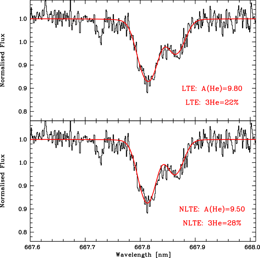
Figure 1: The best fit (solid red) of the helium 667.8 nm line superimposed on the observed HARPS spectrum of Feige 86 (solid black), both for LTE (top) and non-LTE (bottom) line formation.

It would be tempting to use other He i lines to fix the helium abundance, and to fit the 667.8 nm line only to derive the isotopic ratio. It is, however, well known that this line is discrepant with the other He lines, both in LTE and non-LTE (Wolff & Heasley 1985; Smith et al. 1994a, b). Thus the only reasonable approach is to fit the 667.8 nm line with both the He abundance and the isotopic ratio as free parameters.

In Fig.1 we show the observed line and the best fit both in LTE and non-LTE. The derived ³He/⁴He ratios are 22% and 28% respectively; the estimated error of this ratio is 2%.

3 The isotopic ratio of lithium

Lithium is an interesting element, that, according to the standard Big Bang nucleosynthesis (SBBN), is produced in the primordial Universe. It is expected that mainly ⁷Li is produced (⁶Li/⁷Li is predicted to be of the order of $10^{-5}$). Because Li is not supposed to be produced in core-burning nucleosynthesis, it is expected that the Li abundance in old metal-poor stars is closely related to the Li abundance produced by SBBN. In fact, the Li abundance is essentially the same in all metal-poor dwarf stars, irrespective of their temperature and metallicity (the so-called “Spite plateau”, Spite & Spite 1982). There seems to be now a general consensus that these metal-poor stars - as expected from theory - have no 6Li (Cayrel et al. 2007; Steffen et al. 2012; Lind et al. 2013).

The lithium feature at 670.7 nm is a doublet. The line shift between the ⁶Li and the ⁷Li doublet is about 7 km s^-1. The main complication in the derivation of the isotopic ratio is the non negligible thermal broadening of the lines in the stellar atmosphere. For example, for a temperature of 5500 K the full width at half maximum of the Doppler profile is FWHM=6.0 km s^-1 for ⁷Li and FWHM=6.5 km s^-1 for ⁶Li (cf. Cayrel et al. 2007). Thus the doublet is unresolved, and the presence of ⁶Li is signaled by an excess absorption on the red wing of the feature.

In the past, there have been several claims of detection of ${}^{6}{\rm Li}$ (Smith et al. 1998; Cayrel et al. 1999; Asplund et al. 2006), but now it appears that none withstands more sophisticated analysis. The subtleties and possible pitfalls of the derivation of the ⁶Li/⁷Li ratio are described in detail by Cayrel et al. (2007) and Lind et al. (2013) for the case of metal-poor stars. Although these two groups use a slightly different approach, the consistent result is now a non detection of ⁶Li.

Obviously, reliable results can only be achieved with high resolution, high signal-to-noise spectra. In addition, the synthetic spectra used for the line profile fitting must account for the intrinsic line asymmetry that is produced by convective flows in the atmospheres of cool stars and can mimic the presence of ⁶Li. Such analysis requires non-LTE modelling of the lithium line profile, based on 3D hydrodynamical model atmospheres. It has been demonstrated that using 1D LTE instead of 3D non-LTE line profiles leads to a systematic overestimation of the ⁶Li/⁷Li isotopic ratio by up to 2 percentage points (Steffen et al. 2012).

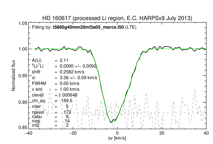
Figure 2: Best fit to the HARPS spectrum of HD 160617 (solid black) with a 1D LTE synthetic spectrum (solid green), indicating a ⁶Li/⁷Li isotopic ratio of $0.0000\pm 0.0092$. The quoted uncertainty is the formal $1\,\sigma$ error of the $\chi^{2}$ fitting procedure, given the signal-to-noise ratio of S/N = $480$ measured on the co-added spectrum (9 sub-exposures with a total integration time of 6.75 h).

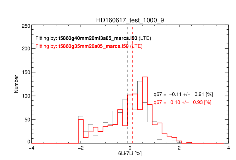
Figure 3: Probability distribution function of the ⁶Li/⁷Li isotopic ratio (in %) obtained from fitting 1000 realizations of the spectrum of HD 160617, generated by bootstrapping from a total of 9 sub-exposures. Two sets of synthetic 1D LTE synthetic spectra were used for this experiment, assuming a gravity of $\log g=4.0$ (black) and $\log g=3.5$ (red), respectively. The standard deviation of the distribution is similar in both cases ($\sigma\approx 0.009$), and fully compatible with the formal $\chi^{2}$ fitting error (Fig. 2).

We re-analyse here the metal-poor star HD 160617, one of the stars for which Asplund et al. (2006) claimed a detection of ⁶Li, based on a 1D LTE analysis of their UVES spectra. This star (5990 K/3.79/–1.76) has a Li abundance on the “Spite plateau”, A(Li)=2.14 (Steffen et al. 2012). We analysed a HARPS spectrum obtained by co-adding nine exposures, four with 1800 s, one with 2700 s, and four with 3600 s exposure time, observed between 2007 and 2012. The analysis on this co-added spectrum gives a non-detection of ${}^{6}{\rm Li}$, both in 1D LTE and 3D non-LTE, in agreement with Steffen et al. (2012) who used only a subset of five of the nine spectra analysed here.

In Fig. 2 the 1D LTE best fit is shown, giving ⁶Li/⁷Li = $0.0000\pm 0.0092$, where the quoted uncertainty is the formal $1\,\sigma$ error of the $\chi^{2}$ fitting procedure for the given the signal-to-noise ratio of S/N = $480$. Fitting with 3D non-LTE synthetic spectra gives a slightly negative (unphysical) isotopic ratio, ⁶Li/⁷Li = $-0.0068\pm 0.0097$.

To obtain an independent estimate of the error of ${}^{6}{\rm Li}/^{7}{\rm Li}$ due to the finite S/N ratio, we analysed a total of 1000 possible realizations of the co-added observed spectrum, each constructed as a sum of nine sub-spectra, drawn randomly (allowing repetitions) from the available set of nine different exposures (so-called bootstrapping). The resulting distribution of the 1000 isotopic ratio determinations is presented as a histogram in Fig. 3. The standard deviation of the distribution is about 0.009, practically the same as the formal $1\,\sigma$ error of the $\chi^{2}$ fitting, suggesting that the latter gives a reasonable estimate of the uncertainty due to the statistical fluctuations in the observed spectra.

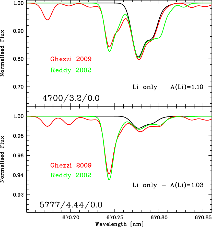
Figure 4: The 1D ATLAS9 / SYNTHE synthetic spectrum in the range of the Li doublet at 670 nm, based on the line list from Reddy et al. (2002) (solid green) and Ghezzi et al. (2009) (solid red), respectively. The contribution of the ⁷Li doublet (solid black) is much stronger for the cool solar-metallicity subgiant (upper panel) than for the Sun (lower panel). The blend line near 670.80 nm in the Reddy et al. list is due to Ti i.

Finally, we point out that, in the case of metal-poor stars, the Li doublet is an isolated feature, and no care has to be taken of possible blending lines. This is no longer true for solar-metallicity stars, and much care has to be devoted to the list of the (metal and molecular) lines falling in the Li spectral range. Unfortunately, the blending lines are not known to the desired precision for an accurate derivation of the Li isotopic ratio. In Fig. 4, we show the synthetic spectrum of the wavelength range around 670.7 nm for the case of the Sun and a solar-metallicity subgiant, based on two different line-lists for the blending lines, as published by Reddy et al. (2002) and Ghezzi et al. (2009), respectively, Obviously, the derived ⁶Li/⁷Li isotopic ratio depends critically on the adopted line list, paricularly for the subgiant.

4 Isotopes of carbon

Carbon is the fourth most abundant element in the Universe, after H, He, and O. Its importance is amplified because it is much easier to detect carbon lines in stellar spectra than oxygen lines, even if oxygen is about two times more abundant than carbon. The main reason for this circumstance are molecular bands of CH (the G-band around 430 nm) and CN (e.g. at 388 nm), easily detectable in stellar spectra. Another reason making C such an interesting element is the discovery, over the last ten years, of ultra iron-poor but carbon enhanced halo stars (see review by Beers & Christlieb 2005).

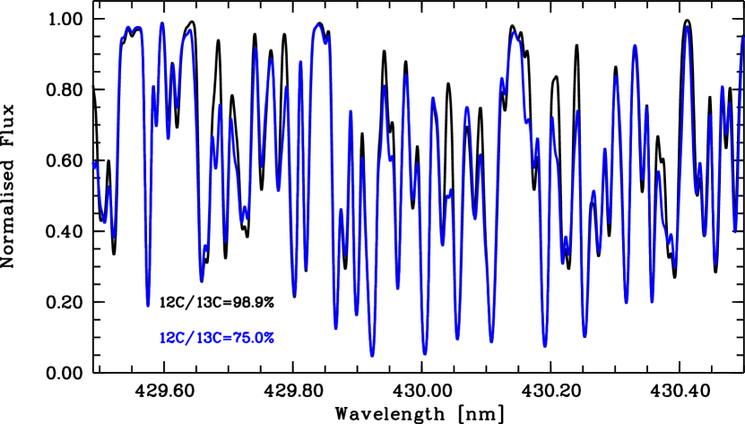
Figure 5: Comparison of two synthetic spectra computed with SYNTHE from an ATLAS model atmosphere with parameters 4595 K/1.1/–2.0. The assumed isotopic ratio is ${}^{12}{\rm C}/^{13}{\rm C}=98.9$% (black), and ${}^{12}{\rm C}/^{13}{\rm C}=75.0$% (blue), respectively. The spectral resolution is compatible with UVES spectra (${\rm R}\approx 80000$).

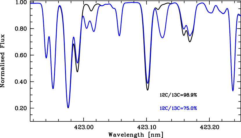
Figure 6: Same as Fig.5, but on the tail of the G-band. Note the isolated ${}^{13}{\rm CH}$ features near 423.01 and 423.12 nm.

The G-band is detectable also at medium (${\rm R}\approx 10000$) to low (${\rm R}\approx 2000$) resolving power, depending on the stellar effective temperature and carbon abundance. However, high spectral resolution is necessary to investigate the carbon isotopic ratio. In Fig. 5 the core of the G-band is shown in the case of a metal-poor giant star for two different ${}^{12}{\rm C}/^{13}{\rm C}$ ratios. In the core of the band, it is obviously very difficult to derive the carbon isotopic ratio. In the tail of the G-band, however, some isolated ${}^{13}{\rm CH}$ lines are accessible and allow an isotopic ratio determination (see Fig. 6).

5 The nickel isotopic ratio in the solar photosphere

Inspired by the work of Brault & Holweger (1981), we analysed the infrared Ni i lines at 1221.6, 1304.8, 1511.6, 1572.6, 1658.4, and 1694.5 nm, to derive the isotopic fraction of ⁵⁸Ni and ⁶⁰Ni. For this purpose, we fitted the observed disc-centre solar spectrum by Delbouille et al. (1981). The grid of synthetic spectra, based on the 1D empirical solar model of Holweger-Müller (Holweger 1967; Holweger & Müller 1974), has been computed with SYNTHE (Kurucz 1993, 2005) in its Linux version (Sbordone et al. 2004; Sbordone 2005). The results are reported in Table 2, and the fits are shown in Fig. 7. Note that the 1694.5 nm line was discarded, because it is heavily blended.

Table 2: Nickel isotopic fractions derived from fitting the solar infrared Ni features, assuming fixed fractions ⁶¹Ni=1.13 %, ⁶²Ni=3.59 %, ⁶⁴Ni=0.91 %.

Wavelength	$\log gf\times$ A(Ni)	58Ni	60Ni	58Ni	60Ni
nm		%	%	%	%
		1D LTE		3D LTE
1221.6	$-0.599\times 6.33$	68.3	26.1	-	-
1304.8	$-1.234\times 6.37$	67.9	26.5	-	-
1511.6	$-0.116\times 5.53$	68.3	26.1	-	-
1572.6	$-1.100\times 6.24$	74.8	19.6	-	-
1658.4	$-0.780\times 6.47$	87.7	6.7	88.5	5.9
1694.5	$-1.417\times 6.92$	-	-	-	-
meteoritic 1)		68.1	26.2

Notes: ¹⁾ Lodders et al. (2009)

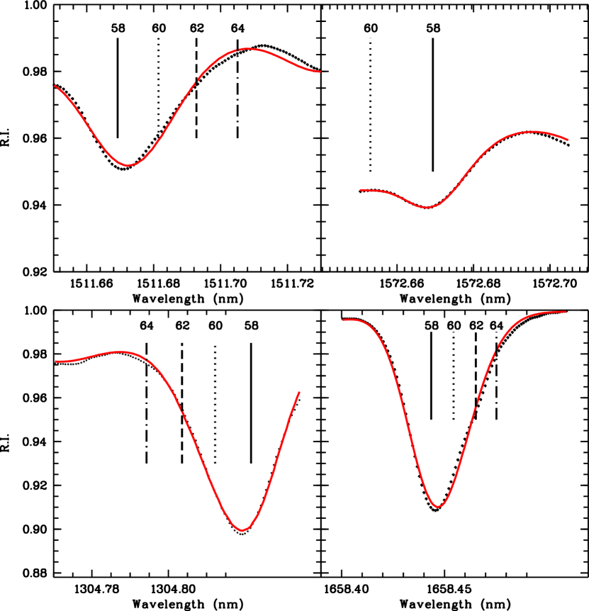
Figure 7: Best fit 1D synthetic profiles (solid red) for 4 Ni lines superimposed on the disc-centre solar spectra (dotted black).

The line at 1658 nm is the cleanest, but yields the highest ⁵⁸Ni fraction. The 1D fit of the red wing is not quite satisfactory. Also, a feature on the red wing suggests an unknown blend, possibly explaining the exceedingly high (super-meteoritic) ⁵⁸Ni fraction derived from this line.

For comparison we computed with Linfor3D a grid of synthetic spectra based on the 3D solar CO⁵BOLD model (Freytag, Steffen, & Dorch 2002; Freytag et al. 2012) used already in previous solar abundance analyses, e.g. in Caffau et al. (2011a, b). The synthetic profile based on the hydrodynamical model is composed of the asymmetric contributions from each of the isotopic components. The result is a feature with an evident asymmetry, the red wing of the 3D profile being stronger than in the 1D profile (see Fig. 8). Figure 9 demonstrates that the 3D profile fits the observed spectrum significantly better than the 1D profile.

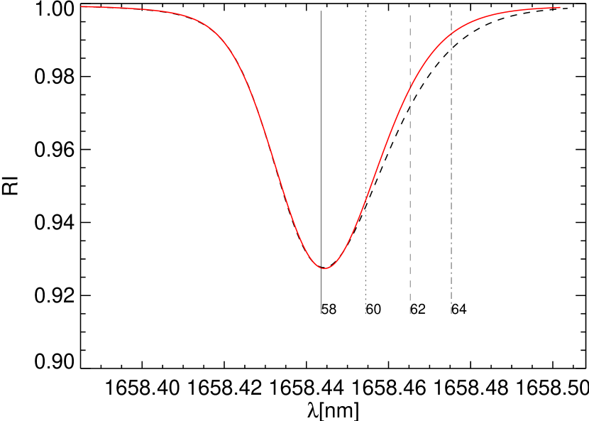
Figure 8: Comparison of the 3D profile (dashed black) with the 1D profile (solid red) of the Ni i line at 1658.4 nm, scaled and shifted to match the blue wing. In both cases, ⁵⁸Ni = 68,1 %, ⁶⁰Ni = 26.2 % (meteoritic). The larger asymmetry of the 3D profile is evident.

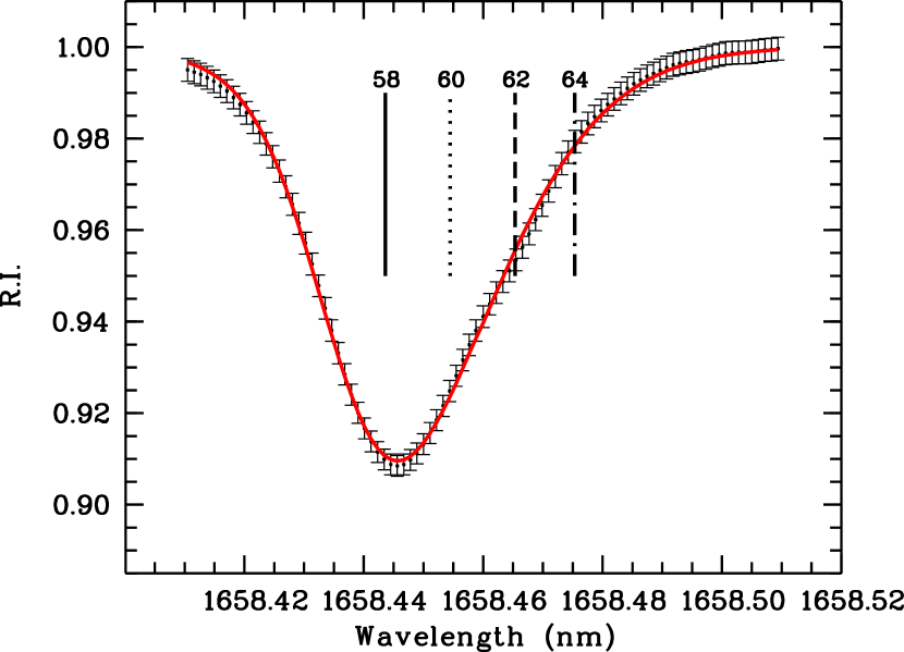
Figure 9: The 3D best fit (solid red) of the Ni line at 1658 nm superimposed on the disc-centre solar spectrum (black symbols).

Nevertheless, the nickel isotopic ratio obtained from the 3D fitting is in good agreement with the one obtained from the 1D fitting based on the Holweger-Müller model (see Tab. 2). This is because the convective line asymmetry affects mainly the outer wing of the profile (see Fig. 8), leaving the shape of the line core essentially unchanged with respect to the 1D case. Since the ⁵⁸Ni to ⁶⁰Ni isotopic ratio influences mainly the line core, due to the small isotopic shift, the derived isotopic fractions are almost insensitive to 3D effects.

6 Conclusions

The knowledge of the isotopic ratios in the chemical composition of a star gives a much deeper insight on the underlying nucleosynthetic processes than just the chemical abundance pattern. However, the analysis of isotopic ratios is demanding both from the observational and theoretical point of view. Good quality data are essential (high-resolution and high signal-to-noise ratio). A precise knowledge of the point source function (PSF) of the spectrograph would certainly improve the analysis, since the shape of the line is crucial in deriving the isotopic ratio for several elements. A laser frequency comb, such as the one tested on the HARPS spectrograph (Wilken et al. 2010; Wilken et al. 2012), would be the ideal tool for measuring the PSF at any desired wavelength. For the HARPS spectrograph, the investigation of the instrumental profile using the laser frequency comb is still ongoing.

In the case of ${}^{6}{\rm Li}/^{7}{\rm Li}$ a resolving power of about 100 000 is necessary with a S/N of at least 600. Only few spectrographs (UVES@VLT, HARPS, HIRES@Keck) can currently provide these quality spectra, especially for metal-poor stars that are usually faint. In the future, we expect a breakthrough with PEPSI@LBT (see Strassmeier et al., this volume), that will allow to reach a resolving power of 300 000, with a fiber-fed echelle spectrograph mounted on a telescope with a 11.8 m equivalent mirror. For the southern hemisphere, ESPRESSO@VLT will provide spectra of similar quality with a resolving power of up to 220 000 (see Molaro et al., this volume).

On the modelling side, we expect the development of grids of new generation 3D model atmospheres, to be utilized for an adequate interpretation of the observed spectra by means of detailed 3D non-LTE synthetic spectra.