High Reynolds number Navier-Stokes solutions and boundary layer separation induced by a rectilinear vortex

Abstract

We compute the solutions of Prandtl’s and Navier-Stokes equations for the two dimensional flow induced by a rectilinear vortex interacting with a boundary in the half plane. For this initial datum Prandtl’s equation develops, in a finite time, a separation singularity. We investigate the different stages of unsteady separation for Navier-Stokes solution at different Reynolds numbers $Re=10^{3}-10^{5}$, and we show the presence of a large-scale interaction between the viscous boundary layer and the inviscid outer flow. We also see a subsequent stage, characterized by the presence of a small-scale interaction, which is visible only for moderate-high Re numbers $Re=10^{4}-10^{5}$. We also investigate the asymptotic validity of boundary layer theory by comparing Prandtl’s solution to Navier-Stokes solutions during the various stages of unsteady separation.

1 Introduction

The aim of this paper is to analyze the unsteady separation process of a 2D incompressible Navier-Stokes (NS) flow induced by the interaction of a point vortex with a physical boundary. We shall solve Navier-Stokes equations at different $Re$ regimes ($Re=10^{3}-10^{5}$) and we shall compare these results with the predictions of the classical Boundary Layer Theory (BLT) as expressed by Prandtl’s equations.

1.1 Prandtl’s equation

Prandtl’s equations can be derived from the Navier-Stokes equations as the formal asymptotic limit for $Re\rightarrow\infty$. It is well known how, for many significant flows, Prandtl’s solutions develop a singularity (see for example [14, 4, 23, 24] and [13, 12]).

In their seminal work devoted to the analysis of the flow around the impulsively started disk, Van Dommelen and Shen [14] found that, in a finite time, a singularity in the Prandtl solution forms (the VDS singularity). The difficulties that had prevented the previous investigations to give reliable results on the singularity, were solved in [14] using a Lagrangian formulation, which allowed to overcome the problem of the growth in time of the normal velocity component $V$ i.e. the growth in time of the boundary layer. More recently the same problem has been tackled in [11, 16, 15] where, using a high resolution Eulerian spectral method, the authors have tracked the VDS singularity in the complex plane before the real blow up of the solution, and have classified it as a cubic-root singularity.

According to the Moore-Root-Sears (MRS) model the singularity in the solution of Prandtl’s equation is related to the unsteady separation of the boundary layer, see also [25]. In fact the occurrence of a singularity means that the normal component of the velocity $V$ becomes infinite with the relative ejection of vorticity and flow particles from within the boundary layer into the outer flow, with the consequent breakdown of the assumptions which Prandtl’s equation are based on.

Before the occurrence of the singularity, the adverse streamwise pressure gradient imposed across the boundary layer induces the formation of a back-flow region. It has been observed that, generally, the formation of a recirculation region corresponds to the vanishing of the vorticity at a point of the boundary. The back flow region grows in time in the streamwise direction, and ejects farther in the normal direction. This results in the formation of a sharp spike in the displacement thickness and in the streamlines. The spike in the streamlines, at the singularity time, reaches the outer external flow, once again a signal of the interaction of the boundary layer with the outer flow.

As an historical remark we mention that before the important results obtained by Van Dommelen $\&$ Shen, the classical definition of unsteady separation was connected with the formation of reversed flow and the vanishing of the wall shear. However Sears and Telionis, in [25], observed that the presence of reversed flow is not in itself sufficient to lead to unsteady separation; they quoted examples of flows with vanishing wall shear for which a breakaway is never expected to occur.

An interesting review on boundary layer theory and on the many numerical experiments which followed Van Dommelen and Shen’s work is given by Cowley in [10]. For the reader interested in the results of the mathematical theory of the Prandtl equations, see [3].

1.2 Navier-Stokes solutions and comparison with BLT

In the rest of the paper we shall denote the Reynolds number with $Re$ defined as:

$$Re=aU_{c}/\nu$$

where $a$ and $U_{c}$ are the distance from the wall and the velocity with respect to the wall of the point vortex, while $\nu$ is the kinematic viscosity. Solving the Navier-Stokes equations at different Reynolds numbers we shall follow the unsteady separation process. We shall find significant differences in the behavior of NS solutions between low ($10^{3}\leq Re\leq 2\cdot 10^{3}$) and moderate-high ($3\cdot 10^{3}\leq Re\leq 10^{5}$) Reynolds number regimes. In fact we shall see how, at different $Re$, different kinds of interactions will establish between the viscous boundary layer and the outer flow; we shall also see that these interactions are the responsible for the ultimate failure of the Prandtl’s equations to give an accurate approximation of the NS flow at the $Re$ numbers we have tested.

In the classical BLT the streamwise pressure gradient is imposed by the outer flow while the normal pressure gradient is zero to leading order. Therefore through the analysis of topological changes of the pressure gradient, we shall be able to distinguish the different stages of the interaction between the BL and the outer flow. Moreover the evolution of the pressure gradient will give indications on the agreement between the Prandtl and the NS solutions.

During the early stage we shall observe that the Prandtl solution is quite close, both qualitatively and quantitatively, to the Navier-Stokes solutions.

On the other hand relevant discrepancies can be observed when the boundary layer flow starts interacting with the outer flow over a large streamwise scale. This event can be related to the formation of an inflection point in the streamwise pressure gradient. This phenomenon is observed for all $Re$ we have considered.

A second different interaction occurring on a smaller scale is present only for moderate-high $Re$ numbers. We notice that, differently from what happens for lower $Re$ numbers, several local maxima-minima form in the streamwise pressure gradient, forcing the formation of several recirculation regions and of strong gradients in the solution. The first appearance of spiky-behavior in the streamlines and vorticity contour level signals the beginning of this new stage. At this time any comparison with Prandtl’s solution fails, even if the formation of large gradients in the solution resembles the terminal singularity stage of Prandtl’s solution. Both types of interaction (large scale and small scale) begin quite early with respect to the first viscous-inviscid interaction that occurs in Prandtl’s solution.

In the literature there are several attempts to incorporate the interaction between the boundary layer and the outer flow in a theory that would improve the classical BLT. We mention the work in [24] where the authors assume that, as the spike in the displacement thickness grows, the outer flow begins to respond to the boundary layer. However the solutions of these Interactive Boundary Layer Theory terminate with a singularity at a time prior to Prandtl’s singularity time. See also [6] and the discussion in [26]. A possible cure to this was proposed in [27] and [20] where the effects of an increasing normal pressure gradient (which is considered constant in the classical BLT) are taken into account. However none of the theories trying to go beyond the classical BLT is fully satisfactory and the problem of a coherent asymptotic theory able to describe the BL separation phenomena is still an open problem, see the discussion in [21] and the review paper [10].

1.3 Plan of the paper

In the next Section we introduce the physical problem, a 2D vortex interacting with a wall, and discuss the regularization procedure we have adopted to treat the relative initial datum. In Section 3 we present the numerical schemes we have used to solve Prandtl’s and Navier-Stokes equations. The numerical results obtained from Prandtl’s equation up to singularity formation are briefly (as this problem was already discussed in great detail in [29, 23]) described in Section 4. In Sections 5 and 6, we show the results obtained for the Navier-Stokes solutions, and we analyze the different stages of unsteady separation. In particular the large-scale interaction stage, that develops for all $Re$ numbers we considered, is discussed in Section 5, while the small-scale interaction stage, found for moderate-high is discussed in Section 6. Our analysis follows the treatment of [4, 21] where the authors studied the interaction of the thick core vortex with a boundary and confirms the scenario described in these paper, as well in [17].

In Section 7 we shall discuss in more detail the physical phenomena leading to the different kind of interactions described in the previous Sections; in particular we shall see first the formation of dipolar vortical structures as the signal of the small scale interaction and second a significant increase in the enstrophy of the flow as the result of the movement of these dipolar structures toward the wall. This analysis is influenced by the findings appeared in a recent series of papers [8, 7, 17] and previously in [22, 9], where the case of the collision of a dipole vortex with a boundary was considered.

2 Statement of the problem

The initial fluid configuration consists of a point-vortex immersed in a 2D viscous incompressible flow at rest at infinity and bounded by an infinite rectilinear wall. The vortex is placed at a distance $a$ from the wall, and is taken with positive rotation and strength $k$. In the inviscid case, the vortex moves to the right parallel to the wall with constant velocity $U_{c}=k/4a\pi$. We refer to [18] for more details.

We introduce a cartesian frame $(x,y)$, such that the $x-$axis coincides with the solid boundary. The point-vortex is centered in $(0,a)$ and we denote by $u$ and $v$ the streamwise and normal velocity components respectively. As in [29, 23], by superimposing a uniform tangential velocity equal and opposite to $U_{c}$, we shall study the system in the frame comoving with the vortex, so that the wall moves with constant velocity $-U_{c}$. We introduce dimensionless variables taking the distance of the vortex from the wall $a$ and the velocity $U_{c}$ as, respectively, characteristic length and velocity.

The governing equations for the flow evolution are the Navier-Stokes equations in the domain $(-\infty,\infty)\times[0,\infty)$ that write as:

$$\frac{\partial u}{\partial t}+u\frac{\partial u}{\partial x}+v\frac{\partial u}{\partial y}+\frac{\partial p}{\partial x} = \frac{1}{Re}\Delta u,$$ (2.1)

$$\frac{\partial v}{\partial t}+u\frac{\partial v}{\partial x}+v\frac{\partial v}{\partial y}+\frac{\partial p}{\partial y} = \frac{1}{Re}\Delta v,$$ (2.2)

$$\frac{\partial u}{\partial x}+\frac{\partial v}{\partial y} = 0\;.$$ (2.3)

The boundary conditions are:

$$u=-1\quad v=0,\qquad\mbox{at}\quad y=0\,,$$ (2.4)

$$u=-1\quad v=0,\qquad\mbox{when}\quad x\rightarrow\pm\infty\,,$$ (2.5)

$$u=-1\quad v=0,\qquad\mbox{when}\quad y\rightarrow\infty\;.$$ (2.6)

The initial data for the velocity components are:

$$u_{0}=\partial_{y}\psi_{E}\quad{\rm and}\quad v_{0}=-\partial_{x}\psi_{E},$$ (2.7)

where

$$\psi_{E}(x,y)=-\log\left(\frac{x^{2}+(y-1)^{2}}{x^{2}+(y+1)^{2}}\right)-y$$ (2.8)

is the streamfunction of the inviscid steady Euler solution for this configuration.

The no-slip boundary condition imposed at the wall leads to vorticity generation at the boundary which develops the unsteady separation phenomenon. To describe the flow inside the boundary-layer, one defines the scaled normal coordinate $Y$ and normal velocity $V$ by the well known boundary layer scaling: $y=\sqrt{Re}Y$ and $v=\sqrt{Re}V$. Prandtl’s equations are obtained, to first order, introducing the above scaling into the Navier-Stokes equations. For the rectilinear vortex case, Prandtl’s equations are:

$$\frac{\partial u}{\partial t}+u\frac{\partial u}{\partial x}+V\frac{\partial u}{\partial Y}-U_{\infty}\frac{\partial U_{\infty}}{\partial x} = \frac{\partial^{2}u}{\partial Y^{2}},$$ (2.9)

$$\frac{\partial u}{\partial x}+\frac{\partial V}{\partial Y} = 0,$$ (2.10)

with initial datum and boundary conditions given by

$$u(x,Y,0)=U_{\infty},$$ (2.11)

$$u(x,0,t)=-1,\quad u(x,Y\rightarrow\infty,t)=U_{\infty},$$ (2.12)

where $U_{\infty}=-1+4/(x^{2}+1)$ is the inviscid solution at the boundary on the reference frame comoving with the vortex.

3 The numerical schemes

3.1 Numerical schemes for Prandtl’s equations

In this section we explain the numerical method used to solve the boundary-layer equations (2.9)-(2.10) with initial and boundary conditions (2.11)-(2.12). This problem was first investigated by Walker in [29], and later by Peridier, Smith and Walker in [23]. The problematic numerical instabilities developed by the numerical method of [29] in Eulerian formulation, were overcome using in [23] a Lagrangian formulation, and using an ADI scheme with upwind-downwind differencing approximation for the convective terms. Probably the use of a central differencing approximation for first derivatives and the lack of the necessary resolution were the main reasons causing instabilities in [29]. Our simulation are based on a Runge-Kutta IMEX scheme for time advancing and on a two step Richtmyer-Lax-Wendroff approximation for the convective terms, which makes possible to carry out the computation almost up to the singularity time in the conventional Eulerian formulation.

Following [4] we shall map the physical domain $(-\infty,\infty)\times[0,\infty)$ onto the finite domain $(-1,1)\times[0,1)$. The map is explicitly given by the following transformations:

$$\hat{x}=\frac{2}{\pi}\arctan{\left(\frac{x-x_{s}}{\alpha}\right)},\qquad\hat{y}=\frac{2}{\pi}\arctan{\left(\frac{Y}{\beta}\right)},$$ (3.1)

being $x_{s}$ the streamwise location where the singularity forms, and $\alpha$ and $\beta$ are positive parameters. These transformations cluster the computational grid close $(x_{s},0)$; the parameters $\alpha$ and $\beta$ determine the degree of focusing of the grid. We note however that as the normal velocity component $V\rightarrow\infty$ as $Y\rightarrow\infty$, we need to truncate the normal domain to a value $Y_{M}$. The value $Y_{M}$ (where the boundary condition $u(x,Y_{M},t)=U_{\infty}$ is imposed) must be big enough so that the growth of the boundary layer does not affect the solution at $Y_{M}$. In our calculation we find that the value $Y_{M}=20$ is enough to ensure the reliability of the computed solution up to times very close to the singularity. Therefore the computational normal domain is $[0,\hat{y}(Y_{M})]$.

Using all these transformation Prandtl’s equations (2.9)–(2.12) become:

$$\frac{\partial u}{\partial t}+u\frac{\partial\hat{x}}{\partial x}\frac{\partial u}{\partial\hat{x}}+V\frac{\partial\hat{y}}{\partial Y}\frac{\partial u}{\partial\hat{y}}-U_{\infty}\frac{\partial U_{\infty}}{\partial x} = \left(\frac{\partial\hat{y}}{\partial Y}\right)^{2}\frac{\partial^{2}u}{\partial\hat{y}^{2}}+\frac{\partial^{2}\hat{y}}{\partial Y^{2}}\frac{\partial u}{\partial\hat{y}},$$

$$\frac{\partial\hat{x}}{\partial x}\frac{\partial u}{\partial\hat{x}}+\frac{\partial\hat{y}}{\partial Y}\frac{\partial V}{\partial\hat{y}} = 0,$$ (3.3)

$$u(\hat{x},\hat{y},0) = U_{\infty},$$ (3.4)

$$u(\hat{x},0,t)=-1,\quad u(\hat{x},\hat{y}(Y_{M}),t) = U_{\infty},$$ (3.5)

$$u(\hat{x}\rightarrow\pm 1,\hat{y},t) = -1.$$ (3.6)

The normal velocity $V$ is computed from the incompressibility equation (3.3) through numerical integration. In Eq.(3.1) the convective term is approximated by the two step Richtmyer-Lax-Wendroff rule (see [19] for details). The diffusive term is approximated by the usual 3-point rule. For the temporal discretization we use the Runge-Kutta IMEX midpoint method (2,3,3) (see [2] for details), and the relative Runge-Kutta tables are:

0 0 0 0

$$\gamma$$ 0 0

0

0

         

0

1/2 1/2

(3.7)

with $\gamma=(3+\sqrt{3})/6$. We have used a grid of $8192\times 2400$ mesh points clustered in ($0.21,0$), and we have set the parameters $\alpha=0.1,\beta=0.1$ in the domain-transformation function (3.1). The time step $\Delta t$ changes at each step according to the CFL condition $\Delta t=\min(\Delta\hat{x}/|u{\partial_{x}\hat{x}}|,\Delta\hat{y}/|V{\partial_{Y}\hat{y}}|)$, where $\Delta\hat{x}$ and $\Delta\hat{y}$ are the tangential and normal mesh sizes. This preserves the computation from any numerical instability until the formation of the singularity.

A different issue (which is present in most of the Prandtl computations presented in the literature) is the incompatibility between the boundary condition at $Y=0$ (2.12) and the initial condition (2.11). The diffusion adjusts this incompatibility in zero time, and in fact our finite-difference code smooths out the discontinuity during the first time step, and no instability occurs. One has to check that the numerical results for the flow evolution do not depend on the way the code smooths out the discontinuity. The procedure we have adopted is the following. We have initiated the flow imposing an initial datum which interpolates smoothly and monotonously between the value of the velocity at the boundary and $U_{\infty}$. The interpolation occurs in a small layer of size $\epsilon$. We have seen that (after a transient) the flow evolution is independent from $\epsilon$, the only difference being a time shift $\Delta T_{\epsilon}$ with respect to the solution obtained imposing the discontinuous initial datum. We have seen that $\Delta T_{\epsilon}\sim\epsilon^{2}$ which is consistent with the fact that the imposition of the artificial interpolation layer has the same effect of the initial diffusive layer. This behavior is independent of the chosen interpolating functions. The same procedure was adopted for the Navier-Stokes solutions.

3.2 Numerical schemes for Navier-Stokes equations

We solve the equations (2.1)–(2.3) in the vorticity-streamfunction formulation:

$$\frac{\partial\omega}{\partial t}+u\frac{\partial\omega}{\partial x}+v\frac{\partial\omega}{\partial y} = \frac{1}{Re}\Delta\omega,$$ (3.8)

$$\Delta\psi = -\omega,$$ (3.9)

$$u=\frac{\partial\psi}{\partial y},\quad v = -\frac{\partial\psi}{\partial x},$$ (3.10)

$$\omega(x,y,t=0)=\omega_{0} = 4\pi\delta_{(0,1)},$$ (3.11)

$$\omega(x\rightarrow\pm\infty,y,0)=\omega(x,y\rightarrow\infty,0) = 0,$$ (3.12)

$$u(x,0,t)=-1,\quad v(x,0,t) = 0.$$ (3.13)

As the initial datum is singular, we convolve with the mollifier $\phi_{\sigma}(x,y)=\frac{1}{\sigma^{2}}e^{-(x^{2}+y^{2})/\sigma^{2}}$, obtaining the regularized initial datum

$${\omega_{0}}_{\sigma}=\omega_{0}\ast\phi_{\sigma}=\frac{4\pi}{\sigma^{2}}e^{-(x^{2}+(y-1)^{2})/\sigma^{2}}\,.$$

We have chosen the value $\sigma=0.05$ and our results do not depend on this particular choice. We have checked that in the boundary layer and up to the computational time $T=1.5$, the differences of the velocity fields between the cases $\sigma=0.05$ and $\sigma=0.025$, are below the precision of the machine.

We have used a stretching function clustering the grid both near the solid boundary and at the point $(0,1)$ where the vortex blob is located. The stretching functions are:

$$\bar{x} = \alpha_{x}\arctan\left(\frac{x-x_{1}}{\beta_{x_{1}}}\right)\left[\gamma_{x}+\arctan\left(\frac{x-x_{2}}{\beta_{x_{2}}}\right)\right],\quad x_{1}<x_{2}$$ (3.14)

$$\bar{y} = \alpha_{y}\arctan\left(\frac{y-y_{2}}{\beta_{y_{2}}}\right)\left[\gamma_{y}+\arctan\left(\frac{y-y_{1}}{\beta_{y_{1}}}\right)\right],\quad y_{1}>y_{2}$$ (3.15)

which map the domain $(-\infty,+\infty)\times[0,\infty)$ in $\left(-\alpha_{x}\frac{\pi}{2}(\gamma_{x}-\frac{\pi}{2}),\alpha_{x}\frac{\pi}{2}(\gamma_{x}+\frac{\pi}{2})\right)\times\left[0,\alpha_{y}\frac{\pi}{2}(\gamma_{y}+\frac{\pi}{2})\right)$. In (3.14) (with analogous meaning for (3.15)) $\beta_{x_{1}}$ and $\beta_{x_{2}}$ are positive parameters tuning the strength of the focusing of the grid points close to $x_{1}$ and $x_{2}$ respectively, $\alpha_{x}$ is a normalizing factor, and $\gamma_{x}$ is a parameter chosen to make the function (3.14) bijective. In particular to have the bijective condition satisfied $\gamma_{x}$ must be chosen so that:

$$\gamma_{x}>\frac{-\beta_{x_{2}}\beta_{x_{1}}^{2}-\beta_{x_{2}}(x-x_{1})^{2}}{\beta_{x_{1}}\beta_{x_{2}}^{2}+\beta_{x_{1}}(x-x_{2})^{2}}\arctan(\frac{x-x_{1}}{\beta_{x_{1}}})-\arctan\left(\frac{x-x_{2}}{\beta_{x_{2}}}\right)\qquad\forall x\,.$$ (3.16)

The value $\gamma_{x}=\gamma_{y}=5$ and $x_{1}=0,y_{1}=1,y_{2}=0$ in (3.14)–(3.15) are kept fixed in all simulations, while the other parameters are listed in Table 1, where it is also reported the typical time-step size we had to adopt to ensure stability of our procedure.

Table 1: Computational parameters.

$Re$	Grid (x,y)	$x_{2}$	$\beta_{x_{1}}$	$\beta_{x_{2}}$	$\beta_{y_{1}}$	$\beta_{y_{2}}$	dt
$10^{3}$	1025$\times$1025	0.4	0.6	0.15	0.2	0.5	$7\cdot 10^{-5}$
$10^{4}$	1025$\times$1025	0.33	0.6	0.1	0.05	0.5	$2\cdot 10^{-5}$
$10^{5}$	4097$\times$1025	0.24	0.65	0.085	0.02	0.4	$2\cdot 10^{-6}$

Applying (3.14)-(3.15) to Navier-Stokes equations (3.8)-(3.11), with the normalizing factors $\alpha_{x}=(\frac{\pi}{2}(\gamma_{x}+\frac{\pi}{2}))^{-1}$ and $\alpha_{y}=(\frac{\pi}{2}(\gamma_{y}+\frac{\pi}{2}))^{-1}$, we obtain this system of equations to be solved in the finite domain $(-\frac{\gamma_{x}-\frac{\pi}{2}}{\gamma_{x}+\frac{\pi}{2}},1)\times[0,1)$

$$\frac{\partial\omega}{\partial t}+\left(\frac{\partial{\bar{x}}}{\partial{x}}u-\frac{1}{Re}\frac{\partial{{}^{2}\bar{x}}}{\partial{x^{2}}}\right)\frac{\partial\omega}{\partial\bar{x}}+\left(\frac{\partial{\bar{y}}}{\partial{y}}v-\frac{1}{Re}\frac{\partial{{}^{2}\bar{y}}}{\partial{y^{2}}}\right)\frac{\partial\omega}{\partial\bar{y}}=$$

$$\frac{1}{Re}\left[\left(\frac{\partial{\bar{x}}}{\partial{x}}\right)^{2}\frac{\partial^{2}\omega}{\partial\bar{x}^{2}}+\left(\frac{\partial{\bar{y}}}{\partial{y}}\right)^{2}\frac{\partial^{2}\omega}{\partial\bar{y}^{2}}\right]\,,$$ (3.17)

$$\left(\frac{\partial{\bar{x}}}{\partial{x}}\right)^{2}\frac{\partial^{2}\psi}{\partial\bar{x}^{2}}+\left(\frac{\partial{\bar{y}}}{\partial{y}}\right)^{2}\frac{\partial^{2}\psi}{\partial\bar{y}^{2}}+\frac{\partial{{}^{2}\bar{x}}}{\partial{x^{2}}}\frac{\partial\psi}{\partial\bar{x}}+\frac{\partial{{}^{2}\bar{y}}}{\partial{y^{2}}}\frac{\partial\psi}{\partial\bar{y}}=-\omega\,,$$ (3.18)

$$\frac{\partial{\bar{y}}}{\partial y}\frac{\partial\psi}{\partial\bar{y}}=u,\qquad\frac{\partial{\bar{x}}}{\partial x}\frac{\partial\psi}{\partial x}=-v\,,$$ (3.19)

$$\omega(x,y,0)=\frac{4\pi}{\sigma^{2}}e^{-(x^{2}+(y-1)^{2})/\sigma^{2}}\,,$$ (3.20)

$$\omega(x\rightarrow\pm\infty,y,0)=\omega(x,y\rightarrow\infty,0)=0\,,$$ (3.21)

$$u(x,0,t)=-1,\qquad v(x,0,t)=0\,.$$ (3.22)

Given that the streamfunction $\psi$ diverges when $\bar{y}\rightarrow 1(y\rightarrow\infty)$, we truncate the physical domain to a value $Y_{max}$ where the vorticity is negligible (up to the computational time). We ran several experiments choosing different value $Y_{max}$, and the value $Y_{max}=10$ was sufficient to avoid any possible dependency.

Regarding advancing in time we have used a factored ADI (Alternating-Direction-Implicit) finite differences approximation, together with a the Crank-Nicolson procedure, which ensures a second order accuracy (see [1]). To find the needed boundary condition for the vorticity at the boundary we have adapted the well known Jensen’s formula to non uniform grids [30]. Finally the Poisson’s equation (3.18) is solved by a $V-cycle$ multigrid iterative method with a standard Gauss-Seidel colouring scheme smoother (see [1, 28]).

4 Prandtl’s solution

In this section we shall give a description of the physical phenomena occurring in the boundary layer leading to the final break up of the solution due to the blow-up of the first derivative of the streamwise velocity component. In particular we shall describe the various stages leading to separation, and focus our analysis on physical events like the formation of the recirculation region and the first viscous-inviscid interaction.

These phenomena were already discussed in [23, 24] and therefore our discussion will be brief and mainly focused on those elements useful for a comparison with the Navier-Stokes solutions. Our results agree with those presented in [23, 24] in the sense that we find all the relevant phenomena related to the separation process (the formation of the recirculation region, the formation of the zero vorticity at the wall and the singularity) to occur at the same times predicted in the mentioned papers.

At early stages the main phenomenon occurring in the boundary layer is the generation of the vorticity at the boundary due to the no-slip boundary condition. At the time $t_{r}\approx 0.28$ the adverse pressure gradient, imposed by the outer flow, leads to the formation of a recirculation region detached from the wall. In fact, the formation of the recirculation region corresponds to the formation of a stagnation point at $(x_{r},y_{r})=(0.74,0.659)$ as consequence of the vanishing of the gradient of the streamfunction $\Psi$, defined here by $\partial_{Y}\Psi=u$. In Fig.1b the recirculation region is clearly visible, at time $t=0.3$, through the presence of a closed streamlines. Notice that the time of creation of a recirculation region does not corresponds to the time of the vanishing of the wall shear $\tau_{w}(x,t)=\frac{\partial u}{\partial Y}_{|Y=0}$, which occurs at $t_{w}\approx 0.337$ in $x_{w}\approx 0.47$ (see Fig.2), i.e. well after the formation of the recirculation region. However this temporal gap disappears if one considers the flow in the laboratory frame where the recirculation region forms exactly at $t=t_{w}$. The recirculation region, as time passes, grows and moves upstream. At $t_{k}\approx 0.85$ a kink forms in the streamlines, above and to the left of the recirculation region, see Fig.1c, due to the pressure gradient that forces the fluid to deflect upward. According to the interpretation given in [23, 24], the formation of the kink represents the first stage of the viscous-inviscid interaction in the boundary layer. In fact, for $t<t_{k}$ before the formation of the kink, the recirculation region, although significantly thickened in the streamwise as well in the normal direction, is still within the boundary layer, close to the wall. For $t>t_{k}$, as the streamwise compression of the flow pushes away fluid particles from the boundary, the flow rapidly focuses in a narrow streamwise region to the left of the recirculation region. This fact reveals how the first stage of the viscous-inviscid interaction occurs. The kink rapidly evolves in a sharp spike which is followed by the singularity formation, due to the blow up of the first derivative of the streamwise velocity component. This final event occurs at time $t_{s}\approx 0.989$ and at the spatial location $x_{s}\approx-0.218$.

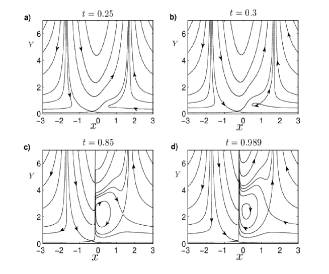
Figure 1: The streamlines of Prandtl’s solution at different times. The recirculation region forms at $t\approx 0.28$, and it is visible in b) at time $t=0.3$. At time $t=0.85$ a kink begins to form in the streamlines as the result of the first interaction of the boundary layer with the inviscid outer flow. At time $t=0.989$ a sharp spike forms in the streamwise location close to $x=-0.218$ as the result of the singularity.

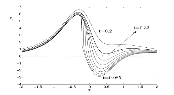
Figure 2: The evolution of wall shear stress starting from time $t=0.2$ up to $t=0.9$ (increments of 0.1) and 0.985. The dotted line is the wall shear at time $t=0.337$ when a region of negative values appears.

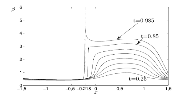
Figure 3: The evolution in time of the displacement thickness from $t=0.25$ up to $t=0.85$ (increments of 0.1) and at $t=0.985$.

The growth of the boundary-layer can be also illustrated through the displacement thickness, which is defined in the laboratory reference frame by:

$$\beta(x)=\int_{0}^{\infty}\left(1-\frac{u+1}{U_{\infty}+1}\right)dY.$$ (4.1)

The time evolution of the displacement thickness is shown in Fig.3 from $t=0.25$ up to $t_{k}=0.85$ (with time-step of 0.1), and at time $t_{s}=0.985$. Up to time $t_{k}$ the displacement thickness grows in correspondence of the growth of the recirculation region. At $t_{k}$ a local maximum (barely visible in the Figure) forms at $x\approx-0.14$, and this signals the onset of interaction of the boundary layer flow with the external flow. Then the boundary layer abruptly focus in a narrow zone close to $x_{s}\approx-0.218$, and at the singularity formation time $t_{s}=0.989$ its normal extension becomes infinite in the boundary-layer scale, leading to the final blow up of the displacement thickness. Moreover the line of zero-vorticity focuses at the same streamwise location as $\beta$ (not shown here). This supports the MRS criterion for the boundary layer breakdown, according to which singularity, and the consequent breakdown of boundary layer assumption, occurs at the zero vorticity line. Physically the singularity formation means that vorticity is ejected in the outer flow from within the boundary layer.

5 Navier-Stokes results: Large-Scale Interaction

In this section we shall study the behavior of the solutions of the Navier-Stokes equations at different $Re$ numbers ($10^{3}-10{{}^{5}}$). We shall also be interested in the comparison between the Navier-Stokes solutions and Prandtl’s solution up to the singularity time $t_{s}=0.989$. In particular we shall investigate the interaction between the viscous boundary layer and the inviscid outer flow occurring during the various stages of the unsteady boundary layer separation.

Before the beginning of this viscous-inviscid interaction the qualitative behavior of the Navier-Stokes solution is similar for all the $Re$ numbers we have considered. The main mechanisms driving the behavior of the flow are the adverse pressure gradients imposed by the vortex and the generation of vorticity at the boundary. In this stage the first relevant phenomenon, visible for all the $Re$ numbers, is the formation of a recirculation region, detached from the wall, underneath and to the right of the central vortex. The recirculation region forms at $t\approx 0.28$, which is in perfect agreement with Prandtl’s solution. The recirculation region starts to thicken both in the streamwise and in the normal direction, and the growth rate depends on the $Re$ number: the larger the $Re$ numbers the slower the recirculation region grows. The wall shear stress $\tau_{w}$, defined here as $\tau_{w}=-\omega_{|y=0}/\sqrt{Re}$, vanishes at time close to $t=0.33$ for all the $Re$ numbers considered, well after the formation of the recirculation region, as we have observed in Prandtl’s solution.

The first relevant discrepancy between the Navier-Stokes and Prandtl’s solutions appears approximately when the viscous-inviscid interaction begins. To analyze this interaction and its influence on the flow evolution, we consider the pressure gradient inside the boundary layer as done in [21, 4] for the thick-core vortex case. In fact for Prandtl’s equation the streamwise pressure gradient does not change as it is imposed by the outer flow, and the normal pressure gradient is always zero. Therefore we shall consider the variations of the pressure gradient of Navier-Stokes equation as an indicator of the discrepancy between the Navier-Stokes and Prandtl’s solutions.

In particular, given that we are mostly interested in the phenomena occurring close to the boundary, we shall focus on the pressure gradient at the wall defined as $\partial_{x}p_{w}\equiv\frac{\partial p}{\partial x}|_{y=0}=-\frac{1}{Re}\frac{\partial{\bar{y}}}{\partial y}\frac{\partial\omega}{\partial\bar{y}}|_{y=0}$. The time evolution of $\partial_{x}p_{w}$ is shown, for different $Re$, in Figs. 4, 5, and 6. As expected, during the early stages of the evolution the pressure gradient experiences only small changes (which are due to the effect of the viscosity), that do not have any remarkable effect on the flow dynamics. However, at a later time (different for different $Re$ numbers) one can observe, close to the maxima, strong variations in the pressure gradients as the result of the first viscous-inviscid interaction. The zone where this interaction acts has streamwise spatial dimension comparable with the characteristic length (the distance of the vortex from the wall) and with the size of the recirculation region, and therefore we call this interaction (as in [4, 21]) the large-scale interaction.

It is not easy to define the precise time when this large-scale interaction begins; in fact, also because the interaction occurs over a wide streamwise scale, it is hard to understand when the variation in $\partial_{x}p_{w}$ has remarkable effects on the flow motion. However one can observe that, in the temporal range during which $\partial_{x}p_{w}$ begins to be visibly different from Prandtl’s streamwise pressure gradient, there is the formation of a pair of inflection points between the maximum and the inflection point located in $(0,0)$. These two inflection points are the consequence of the vanishing of the second derivative of $\partial_{x}p_{w}$ and forms at time $t\approx 0.34$ for $Re=10^{3}$, $t\approx 0.38$ for $Re=10^{4}$ and $t\approx 0.47$ for $Re=10^{5}$, at the spatial locations $x\approx 0.29$, $x\approx 0.2$, $x\approx 0.17$ respectively. These inflection-points carry physical meaning, as they are the precursor of the formation of local minima in the pressure gradient which will eventually become negative (see e.g. Fig.11b of the next Section for the case $Re=10^{3}$). These local negative minima in $\partial_{x}p_{w}$ reflects a pressure gradient adverse to the flow motion in the primary recirculation region near the wall, which forces the formation of a secondary recirculation region, and introduces a change in the qualitative behavior of the flow. For this reason we define the time when large-scale interaction begins as the time when these inflection point forms in $\partial_{x}p_{w}$. At this time one can observe significant quantitative differences between Prandtl’s and Navier-Stokes solutions.

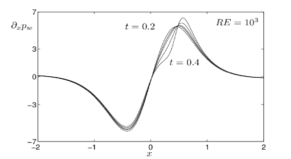
Figure 4: Evolution in time, from $t=0.2$ up to $t=0.4$ (with increments of 0.05), of the streamwise pressure gradient on the wall. Reynolds number is $Re=10^{3}$. The local change close to the maximum is the result of the large-scale interaction.

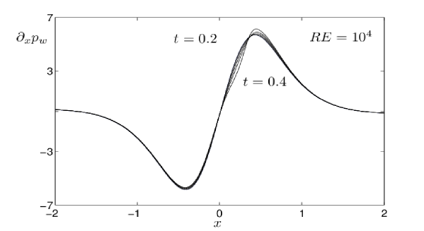
Figure 5: Evolution in time, from $t=0.2$ up to $t=0.4$ (with increments of 0.05), of the streamwise pressure gradient on the wall. Reynolds number is $Re=10^{4}$. The local change close to the maximum is the result of the large-scale interaction.

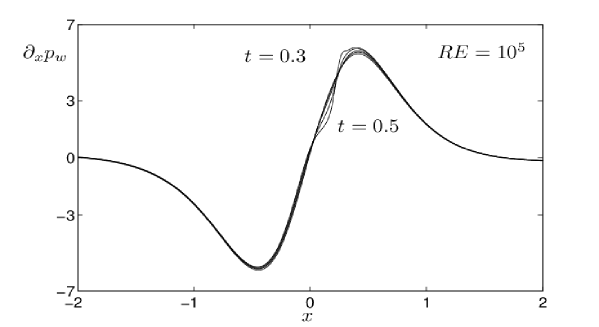
Figure 6: Evolution in time, from $t=0.3$ up to $t=0.5$ (with increments of 0.05), of the streamwise pressure gradient on the wall. Reynolds number is $Re=10^{5}$. The local change close to the maximum is the result of the large-scale interaction.

In Fig.7 we show the behavior of the wall shear stress (which is basically the vorticity at the wall) for Prandtl’s solution and Navier-Stokes solutions for different $Re$. The most visible differences are evident during the large-scale interaction stage in all cases. For $Re=10^{3}$ (Fig.7a) Navier-Stokes and Prandtl’s wall shear are very close up to time $t=0.3$, reflecting the good agreement between the two solutions in the whole boundary layer. On the other hand at time $t=0.4$ one can already see significant discrepancies, and these are the consequence of the large-scale interaction influencing Navier-Stokes solution. This influence is also shown for $Re=10^{4},10^{5}$ in Figs.7b,c at $t=0.4$ and $t=0.5$ respectively.

We conclude this Section stressing how the discrepancies between the Navier-Stokes and Prandtl’s solutions during this stage are merely quantitative, while the overall qualitative properties of the two flows are quite similar. In fact during the large-scale interaction only one big recirculation region is present in the NS flow (likewise in classical BLT). Moreover the magnitude of the normal pressure gradient re-scaled according to the boundary layer variable ($\partial_{Y}p=Re^{-1/2}\partial_{y}p$) is of order $O(Re^{-1/2})$. This is compatible with the Boundary Layer assumption predicting that the normal pressure gradient is always zero. This is shown in Fig.8 where one can see the evolution in time of $||\partial_{y}p||_{\infty}$ evaluated inside the boundary layer.

It is therefore clear that the large scale interaction has a different character compared with the viscous-inviscid interaction visible in Prandtl’s flow. The latter, in fact, which is signaled by the rapidly growth of the spike in the streamlines, begins at the time $t_{k}=0.85$ while, at least for the $Re$ considered here, the large-scale interaction begins at times between $0.3$ and $0.5$. More importantly, during the large-scale interaction no large gradient is present and the flow remains confined in the boundary layer without eruption toward the outer flow. These phenomena characterize the following stage of the evolution and will be analyzed in the next Section.

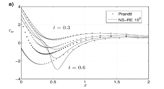
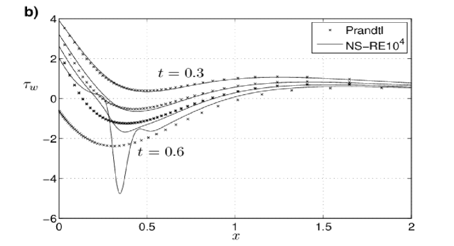
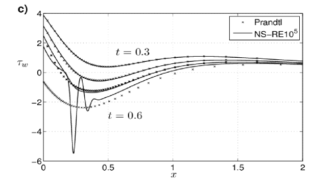
Figure 7: A comparison in time between Prandtl and Navier-Stokes wall shear for various $Re$ numbers . The comparison starts at time $t=0.3$ up to time $t=0.6$ (increments of 0.1). They compare well up to when the large-scale interaction begins, which happens at $t=0.34,0.38,0.47$ for $Re=10^{3},10^{4},10^{5}$ respectively.

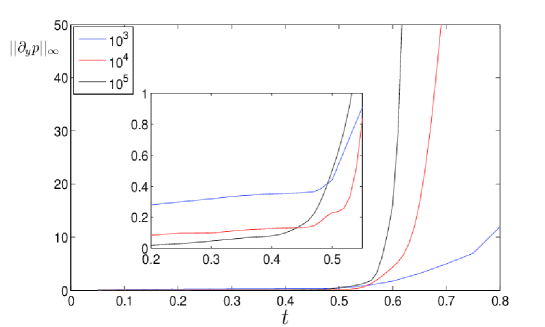
Figure 8: The evolution in time of the sup norm of $\partial_{y}p$ in the boundary layer from time 0.2 to 0.8. In the inset the evolution from 0.2 to 0.6. Note how $Re^{-1/2}\partial_{y}p$ remains of order $O(Re^{-1/2})$ during the whole large-scale interaction stage.

6 Navier-Stokes results: Small-Scale Interaction

The characteristics of the large-scale interaction bear no resemblance with the viscous-inviscid interaction developed by Prandtl’s solution which is characterized by the formation of a spike in the streamlines and vorticity contours. However the large-scale interaction in Navier-Stokes solutions is the precursor of another interaction, acting on a smaller scale. We shall see that this phenomenon occurs only for moderate-high $Re$ (i.e. $10^{4}\leq Re\leq 10^{5}$) numbers.

6.1 Moderate-high Reynolds numbers: $10^{4}\leq Re\leq 10^{5}$

To describe this new interaction in Fig.9a we show, for $Re=10^{4}$, the streamlines at time $t=0.56$, while in Fig.9b we show the wall shear $\tau_{w}$ (dotted) and the streamwise pressure gradients on the wall $\partial_{x}p_{w}$ (dashed). In the streamlines it is clearly visible the formation of a kink located above and to the left of the recirculation region; in correspondence one can observe a strong streamwise variation in $\tau_{w}$ and $\partial_{x}p_{w}$ and the rapid alternation of critical points. The first minimum of $\partial_{x}p_{w}$ forms on the left of the main maximum (the time at which the minimum appears is roughly $t\approx 0.52$) at $x\approx 0.21$, close to the streamwise location where we observed (in the previous Section) the change of concavity that characterizes the large-scale interaction. At time $t\approx 0.56$ this minimum becomes negative; one therefore has a pressure gradient that is adverse with respect to the flow motion of the recirculation region close the boundary. In Fig.9b one observes that the minimum in the pressure gradient is followed, through a sharp increase, by a positive maximum (where the pressure gradient is therefore favorable). The fluid portion between the minimum and the maximum is therefore strongly compressed in the streamwise direction. This compression accelerates the evolution of the kink (visible in Fig.9a) in a spike (visible in Fig.9c), and it is the responsible for the growth in the normal direction of the boundary layer, and of the subsequent vorticity eruption. The presence of the kink and of the subsequent spike signals a new kind of interaction between the BL and the outer flow, which is called small scale interaction, [21].

Notice also, in Fig.9b, the presence of a second local minimum which forms at $x\approx 0.49$. This secondary minimum will soon become negative (see Fig.9d), with the consequent presence of a further adverse pressure gradient; this leads to the splitting of the recirculation region in two recirculation regions which is clearly visible in Fig.9c. On the other hand the primary minimum in the pressure gradient, which in Fig.9d is located at $x\approx 0.28$, creates an adverse pressure gradient: this creates the conditions for the birth of a further recirculation region attached to the boundary, which is visible in Fig.9e.

The newly created recirculation region, pushing the fluid from below, causes a further splitting of the primary recirculation region, visible in Fig.9g. The process of creation of vortical structures continues over and over, while the structure of the pressure gradient becomes more and more complicated. This can be seen in Figs.9i-l.

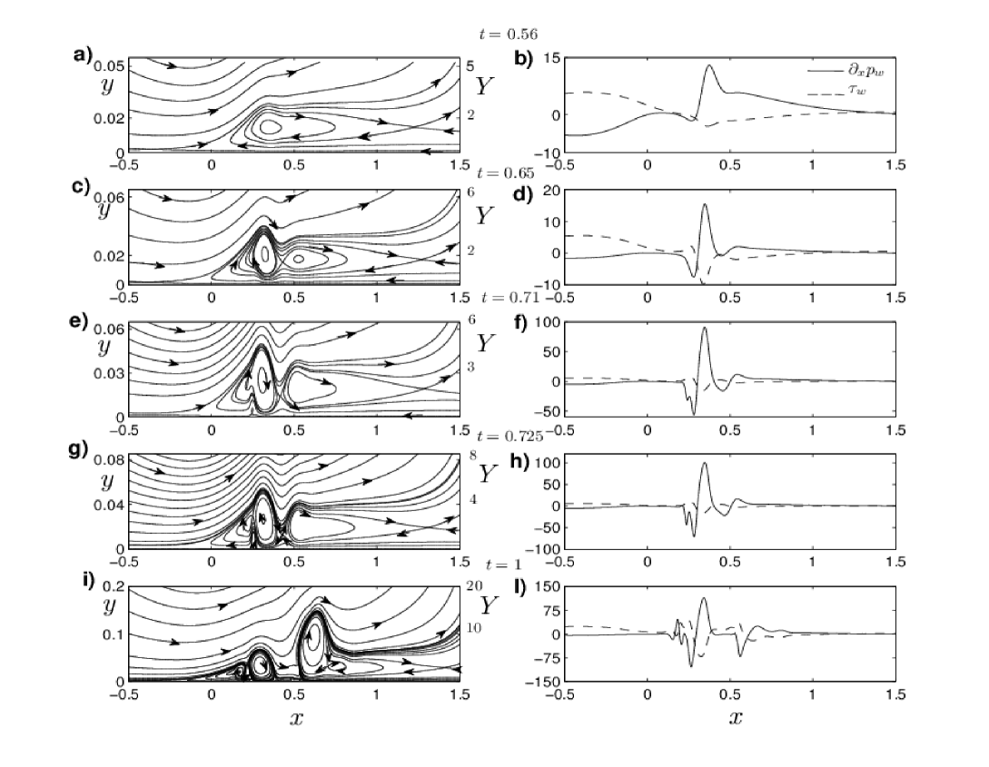
Figure 9: $Re=10^{4}$. Streamlines on the left, wall shear stress (dotted) and streamwise pressure gradient on the wall (dashed) on the right. At $t=0.56$ a kink is visible above and to the left of the recirculation region. This kink corresponds to the formation of a negative minimum (upstream respect to the near wall flow motion) and a positive maximum (downstream) of the streamwise pressure gradient. The splitting of the recirculation region, caused by the presence of alternating adverse-favorable-adverse pressure gradients, is visible at $t=0.65$. A new recirculation region is visible at $t=0.71$ due to the adverse pressure gradient created by the minimum to the left of the main maximum. At $t=0.725$ this new recirculation region causes a further splitting of the primary recirculation region. At $t=1$ several eddies are visible and the splitting of the recirculation regions continues.

The behavior for $Re=10^{5}$ is qualitatively similar the main difference being that the whole sequence of formation of alternating critical points in the pressure gradient followed by the splitting of the recirculation region is considerably faster. In fact the first downstream minimum in the pressure gradient forms at $t\approx 0.52$ in $x\approx 0.3$, while the second upstream minimum forms at time $t\approx 0.53$ in $x\approx 0.13$. All this is clearly visible in Fig.10.

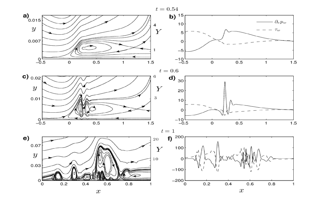
Figure 10: $Re=10^{5}$. Streamlines on the left, wall shear stress (dotted) and streamwise pressure gradient on the wall (dashed) on the right. The kink on the streamlines visible at $t=0.54$ is the result of the formation of an upstream and downstream minimum in $\partial_{x}p_{w}$. At $t=0.6$ the recirculation region is split caused by the presence of alternating adverse-favorable-adverse pressure gradients. At $t=1$ complicated structures are present in the flow.

6.2 Low Reynolds numbers: $Re\simeq 10^{3}$

For $Re=10^{3}$ the flow evolution is quite different from what we have seen for $Re=10^{4}-10^{5}$. In fact after the large-scale interaction stage only the upstream minimum forms at $t\approx 0.49$ in $x\approx 0.28$; this minimum becomes negative at time $t\approx 0.54$ in $x\approx 0.35$. The splitting of the recirculation region happens at $t=0.95$ on the left side of the primary recirculation region, and a secondary recirculation forms underneath the primary soon after $t=1$ as consequence of the adverse pressure gradient to the recirculation flow motion. In Fig.11 we show the streamlines, the wall shear and the streamwise pressure gradient at the wall at time $t=1.02$: no formation of any local minimum downstream to the right of the local maximum is present, no kink or spike in the streamlines, and no large gradients in $\partial_{x}p_{w}$ or $\tau_{w}$. Therefore the typical characterizations of the small-scale interaction are not present for $Re=10^{3}$. We have checked that, up to time $t=6$, no small-scale interaction can be detected.

The different flow evolution observed for $Re=10^{3}$ can be explained with the larger diffusive effects acting for lower $Re$ number, which prevents the streamwise compression that, for $Re=10^{4}-10^{5}$ led to the formation of the spike. This difference can be seen also in terms of pressure gradient; in fact no minimum in $\partial_{x}p_{w}$ forms downstream and the pressure gradient keeps the rather simple structure visible in Fig.11b. Clearly the formation of the local downstream minimum is a crucial event in the flow evolution, as it causes an early splitting of the recirculation region and initiates the cascade of eddies that characterizes the moderate-high $Re$ regime.

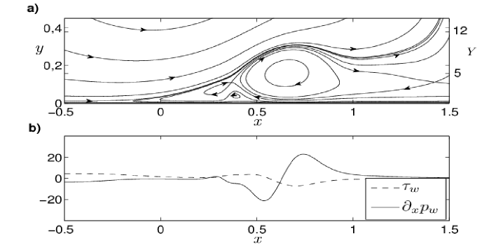
Figure 11: $Re=10^{3}$, t=1.02. a) streamlines. b) wall shear (dotted), streamwise pressure gradient at the wall (dashed). The primary recirculation region splits in two co-rotating eddies, and a new recirculation region forms underneath soon after $t=1$.

The boundary between the low Reynolds number regime and the moderate-high regime is in between $Re=2\cdot 10^{3}$ (for this $Re$ we have not detected the small scale interaction) and $Re=3\cdot 10^{3}$ (for which, on the other hand, the small-scale regime is visible).

7 Separation, dipolar structures and vorticity production

The description of the unsteady separation of the previous sections was based on the analysis of the evolution of the streamwise pressure gradient and of the vorticity at the wall. In this Section we shall look at the boundary layer dynamics from a different perspective. Namely we shall see how, for moderate-high $Re$, an important event occurring during the separation process, is the creation of several vortex-dipoles, and that the reciprocal interaction between these structures leads to a sharp increase in the enstrophy of the flow.

The equations for the evolution of the energy and of the enstrophy of the flow within the boundary layer $D$ (see Section 3.2 for the definition of $D$) write as:

$$\frac{dE(t)}{dt} = -\frac{1}{Re}\Omega(t)+I^{\omega}(t)+NT_{1}$$ (7.1)

$$\frac{d\Omega(t)}{dt} = -\frac{2}{Re}P(t)+2I^{p}(t)+NT_{2}$$ (7.2)

where

$$I^{\omega}(t) = -\frac{1}{Re}\int_{-\infty}^{+\infty}u_{y=0}\cdot\omega_{|y=0}dx\,,$$

$$I^{p}(t) = \int_{-\infty}^{+\infty}\omega_{|y=0}\cdot\partial_{x}p_{w}dx\,,$$

and

$$NT_{1} = {-\frac{1}{2}\int_{\partial D}\mathbf{u}^{2}(\mathbf{u}\cdot\mathbf{n})dl}-\int_{\partial D}p(\mathbf{u}\cdot\mathbf{n})dx-\frac{1}{Re}\int_{-\infty}^{\infty}(\omega u)|_{y=Y_{BL}}dx\;,$$

$$NT_{2} = \frac{2}{Re}\int_{-\infty}^{+\infty}\left(\omega\cdot\partial_{y}\omega\right)_{|y=Y_{BL}}dx\;,$$

being $\mathbf{n}$ the exterior normal to $\partial D$. The $NT_{i}$ terms are negligible because at $y=Y_{BL}$ the vorticity $\omega$ is very small and the normal component of the velocity is very close to be an odd function while $\mathbf{u}^{2}$ and $p$ are even. We shall not consider these terms in the rest of our analysis.

The energy decreases, as the negative term due to the enstrophy is larger than $I^{\omega}(t)$ (see Figs.16b-d). From (7.2) one can see that the only way for the enstrophy to increase is via the integral term $I^{p}$ which is related to the vorticity and to the vorticity flux at the boundary. We shall see that the enstrophy within the boundary layer can in fact increase, and how the evolution in time of $\Omega(t)$ is related to important events characterizing the separation process.

7.1 Large-scale interaction: the detachment of boundary layer

Prior to the large-scale interaction the flow evolution is almost the same for all the $Re$ numbers. The no-slip condition at the wall stops the flow motion and creates a boundary layer of negative vorticity $BL_{-}$. At $t\approx 0.33$ the adverse pressure gradient imposed by the primary vortex leads to the formation of a positive vorticity zone $b_{1+}$ under $BL_{-}$. This situation is visible in Figs.12 for $Re=10^{3}$, where the positive vorticity $b_{1+}$ still remains beneath $BL_{-}$ at $t=1$ and $t=1.5$. As time passes, the part of $BL_{-}$ located to the right of the primary vortex, rolls-up and moves to the right due to the velocity imposed by the primary vortex itself, being also pushed up by the positive vorticity zone $b_{1+}$. As $BL_{-}$ detaches from the wall, it creates a clockwise rotation close to the wall, and therefore the flow particles, especially those in $b_{1+}$, are accelerated from right to left. Therefore the streamwise pressure gradient becomes negative on the left of the core of $BL_{-}$, creating an adverse pressure gradient to the recirculation region, see for example Fig.9. This variation in the streamwise pressure gradient is gradual, and it is a direct consequence of the detachment process of the boundary layer $BL_{-}$, which begins to interact with the inviscid outer flow leading to the large–scale interaction stage described in Section 5.

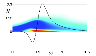
(a) $Re=10^{3},t=.65$

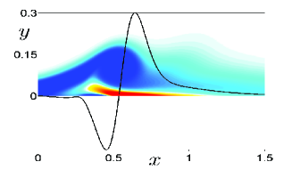
(b) $Re=10^{3},t=.80$

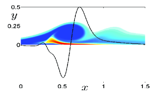
(c) $Re=10^{3},t=1.0$

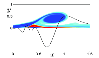
(d) $Re=10^{3},t=1.5$

Figure 12: Vorticity contour levels for $Re=10^{3}$ at different times compared with $\partial_{x}p_{w}$ (rescaled to fit the normal extension of vorticity). The blue colors represents negative vorticity, red/yellow positive vorticity.

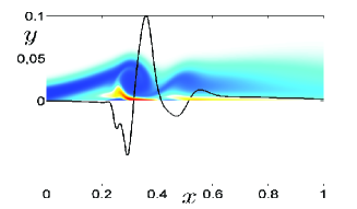
(a) $Re=10^{4},t=0.7$

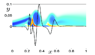
(b) $Re=10^{4},t=0.78$

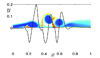
(c) $Re=10^{4},t=0.9$

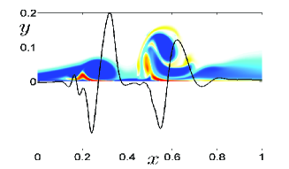
(d) $Re=10^{4},t=0.98$

Figure 13: Vorticity contour levels for $Re=10^{4}$ at different times compared with $\partial_{x}p_{w}$ (rescaled to fit the normal extension of vorticity). The blue colors represents negative vorticity, red/yellow colors the positive vorticity.

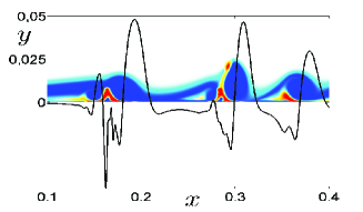
(a) $Re=10^{5},t=0.68$

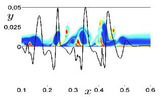
(b) $Re=10^{5},t=0.72$

Figure 14: Vorticity contour levels for $Re=10^{5}$ at $t=0.68$ and $t=0.72$ compared with $\partial_{x}p_{w}$ (rescaled to fit the normal extension of vorticity). The blue colors represent negative vorticity, red/yellow colors positive vorticity

7.2 Small-scale interaction: the formation of vortex dipoles

The detachment process after the large-scale interaction strongly depends on the $Re$ number. In Section 6.1 we have described the flow evolution for moderate-high $Re$ numbers. This regime is characterized by the evolution of the large-scale interaction in the small-scale interaction and by the formation of several recirculation regions on a small spatial scale. To explain the physical features leading to small-scale interaction, we shall focus mainly on the case $Re=10^{4}$, as it is simpler to describe than $Re=10^{5}$.

From the detachment process of the boundary layer, a core of negative vorticity $B_{1-}$ emerges and rotates clockwise in the boundary layer. This core of negative vorticity forms at $t\approx 0.63$ and it is clearly visible at $t=0.7$ in Fig.13a centered in $(0.29,0.023)$. The vortex $B_{1-}$ forms a dipolar structure with the positive vorticity $b_{1+}$, creating a favorable condition for the vorticity production at the wall. It is interesting to notice how $B_{1-}$ has enough strength to give a spin to the positive vorticity $b_{1+}$, which elongates around $B_{1-}$ and penetrates in the zone of negative vorticity, see Fig.13b. During this movement, $b_{1+}$ breaks in two parts; the weaker part, that from now on we shall denote with $b_{2+}$, remains connected to the wall. At time $t\approx 0.68$, a new core of negative vorticity, $B_{2-}$ (visible in Fig.13 for all time), is created on the right of $B_{1-}$, and it forms a second dipolar structure with $b_{2+}$. Moreover, from the detachment process of the first dipolar structure, given by the coupling of $B_{1-}$ and $b_{1+}$, a third dipolar structure forms on the left of $B_{1-}$, at $t\approx 0.75$, visible in Figs.13b-d at $t=0.78,0.9$ and $t=0.98$. The mutual interaction of these dipolar structures results in the movement toward the wall of the negative vortex cores $B_{1-}$ and $B_{2-}$. This movement has a striking effect on the evolution in time of $\Omega(t)$ which rapidly increases showing a first peak at $t\approx 0.78$, see Fig.16b. In fact at this time the distances from the wall of the centers of $B_{1-}$ and $B_{2-}$ (see Figs.15a-b) reach a local minimum, and the positive vorticity $b_{1+}$ and $b_{2+}$ are squeezed under $B_{1-}$ and $B_{2-}$, leading to the production of a large amount of vorticity at the wall with is signaled by growth of $I^{p}(t)$ visible in Fig.16a.

The next peak in $\Omega(t)$ form at $t\approx 0.98$ when the first dipolar structure strongly interacts with the second and pushes it close to the wall, as shown in Fig.13d near $x=0.6$. At this time, the center of $B_{2-}$ (see Fig.15b) reaches a new minimal distance from the wall, squeezing the zone of positive vorticity $b_{2+}$ under $B_{2-}$. Subsequently, the two dipolar structures merge together and move upward to finally interact with the primary vortex.

The phenomena characterizing the dynamic of flow evolution for $Re=10^{4}$ are also visible for $Re=10^{5}$, but in this case the formation of vortices and dipolar structures within the boundary layer is much more chaotic and difficult to describe. Also for $Re=10^{5}$ the peaks in $\Omega(t)$, shown in Fig.16b, correspond to the impingements of the dipolar structures on the wall. Similarly to the case $Re=10^{4}$, the first peak in $\Omega(t)$ corresponds to the time when $B_{1-}$ gets closer to the wall. This event happens at $t\approx 0.68$, when other several dipolar structures are also present, as visible in Fig.14a. The second peak of $\Omega(t)$ is reached at $t\approx 0.72$, when, similarly to the case $Re=10^{4}$, a dipolar structure near $x=0.45$ (see Fig.14b) is pushed close to the wall due to the interaction with another dipolar structure; at this time eight cores of negative vorticity are clearly visible. Hereafter $\Omega(t)$ reaches several other peaks, as a consequence of the complicated dynamics of the flow.

The effects of the small-scale interaction are therefore related to the formation of the peaks in $\Omega(t)$. The first peak forms earlier for $Re=10^{5}$ than for $Re=10^{4}$, confirming that the large-scale interaction accelerates the small-scale interaction formation as the $Re$ number increases.

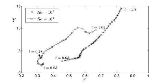
(a) Trajectory of vortex $B_{1-}$ for $Re=10^{3},10^{4}$. The trajectory for $Re=10^{3}$ is followed from $t=0.65$ to $t=1.5$ with temporal step of 0.2. The trajectory for $Re=10^{4}$ is followed from $t=0.63$ to $t=1.05$ with temporal step of 0.1.

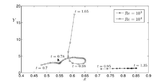
(b) Trajectory of vortex $B_{2-}$ for $Re=10^{3},10^{4}$. The trajectory for $Re=10^{3}$ is followed from $t=0.95$ to $t=1.35$ with temporal step of 0.4. The trajectory for $Re=10^{4}$ is followed from $t=0.7$ to $t=1.05$ with temporal step of 0.1.

Figure 15: The trajectory of vortex $B_{1-}$ and $B_{2-}$ for $Re=10^{3},10^{4}$.

The flow evolution for the case $Re=10^{3}$ is totally different from the cases $Re=10^{4},10^{5}$. In fact, for $Re=10^{3}$, the viscosity makes the primary dipolar structures weaker than the ones observed in the cases $Re=10^{4},10^{5}$. Like in $Re=10^{4},10^{5}$, a core $B_{1-}$ of negative vorticity emerges within the boundary layer at $t\approx 0.65$, forming the first dipolar structure with the positive vorticity zone $b_{1+}$. This structure is clearly visible in Fig.12. However, because of its weakness, $B_{1-}$ is not able to elongate the positive vorticity $b_{1+}$ around $B_{1-}$, as seen for $Re=10^{4}-10^{5}$, and this also prevents the break up of $b_{1+}$ and the subsequent formation of other dipolar structures. In fact, even if two other cores of negative vorticity $B_{2-}$ and $B_{3-}$ emerge on the right and on the left of $B_{1-}$ at $t\approx 0.95$ and $t\approx 1.06$ respectively, they cannot pair with other cores of positive vorticity, preventing the interaction between the dipolar structures that were responsible for the formation of the peaks in $\Omega(t)$ for $Re=10^{4}-10^{5}$.

In Fig.15 one can also observe how the centers of $B_{1-}$ and $B_{2-}$ never move toward the wall, preventing the growth of $\Omega(t)$. At time $t=1.5$, $B_{1-}$ has significantly moved away from the wall and it is going to interact with the primary vortex. One can observe that the only relevant effects related to the formation of $B_{2-}$ are the small peaks in $I^{p}(t)$ and $P(t)$ that, however, combined in (7.2) are not sufficient to increase the enstrophy in the boundary layer.

In Fig.16 we report the enstrophy and the palinstrophy (and the related quantities $I^{p}$ and $I^{\omega}$) of NS solutions rescaled as:

$$\tilde{I}^{p}=I^{p}/Re^{1/2},\;\tilde{\Omega}=\Omega/Re^{1/2},\;\tilde{P}=P/Re^{3/2},\tilde{I}^{\omega}=I^{\omega}Re^{1/2}\,.$$ (7.3)

as well the same quantities for Prandtl’s solutions.

The physical condition leading to the growth in time of the enstrophy is therefore the impingement on the wall of the negative part of the dipolar structures, similarly to what has been shown in [7, 8, 17] and previously in [9, 22], where the authors studied the interaction of a vortex dipole with a no-slip boundary. This set-up differs substantially from the case described in this paper and from the case of the thick core vortex analyzed in [21]. In fact, if the dipole is sufficiently far from the wall, the flow evolution does not differs noticeably from the free-slip or the stress-free case and a very weak boundary-layer forms at $t=0$. The boundary layer detachment derives from the movement toward the wall of the dipole, which also leads to the formation of an adverse pressure gradient at the wall, differently from our case where the adverse pressure gradient is instantly imposed by the primary vortex. However this detachment process also shows significant similarities with our case. In fact in [17], two different $Re$ number regimes were detected: for $Re>O(10^{4})$ a shear instability forms in the boundary-layer before it detaches from the wall, leading to the roll-up of the boundary layer and to the formation of small-scale vortex-structures, with large amount of vorticity production. For $Re<O(10^{4})$, instead, no small-scale interaction was detected, and the boundary layer detaches from the wall forming single vortices which totally wrap-around the dipole halves. Moreover for all the $Re$ regimes, during the various rebounding of the dipolar structures on the wall, the enstrophy increased when the dipoles get close to the wall, similarly to what happens in our case.

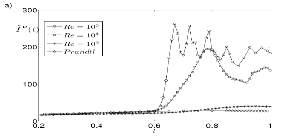
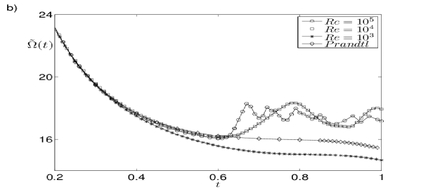
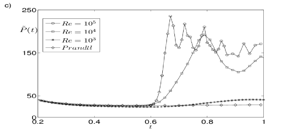
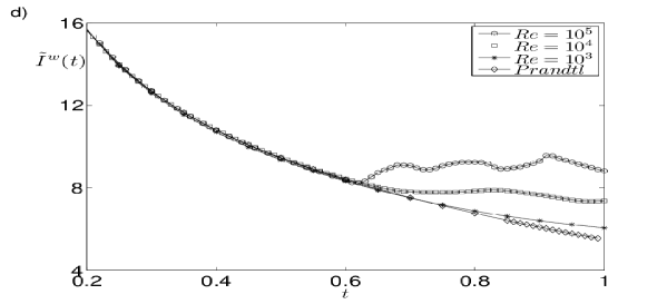
Figure 16: A comparison between $I^{p}_{P}(t)$, $\Omega_{P}(t)$, $P_{P}(t)$, $I^{w}_{P}(t)$ and $I^{p}(t)$, $\Omega(t)$, $P(t)$, $I^{w}(t)$ at different $Re$ rescaled according to (7.3). Up to large-scale interaction the good comparison reflects the good agreement between NS and Prandtl’s solutions. During the small-scale interaction (only for $Re=10^{4}-10^{5}$) the values for NS strongly differ from Prandtl due to the interactions of the dipolar structures within the boundary layer.

8 Conclusions

We have computed the solutions of 2D Prandtl and Navier-Stokes equations in the case of a rectilinear vortex interacting with a wall. We have analyzed the asymptotic validity of boundary layer theory by comparing Prandtl’s solution with the NS solutions for $Re$ in the range $10^{3}-10^{5}$. In our case Prandtl solution terminates in a singularity at time $t\approx 0.989$. The singularity formation is anticipated by a first interaction of the boundary layer flow with the outer flow, which is revealed by the spiky behavior of the streamlines and of the displacement thickness at $t\approx 0.85$. This is the consequence of the compression of the flow in the streamwise direction in a very narrow zone, which leads to an eruption in the normal direction with ejection of flow from within the boundary layer to the outer flow at singularity time.

The unsteady separation process, as predicted by the NS equations, has a different evolution, at least for the $Re$ regimes considered here. In fact, we have seen a good quantitative agreement between Prandtl and NS solution only during the earlier stages, until the beginning of the large-scale interaction, which is signaled by the local change of the streamwise pressure gradient in the boundary layer. This interaction starts later the higher the $Re$ number, and acts over the flow in a region close to the boundary whose size, in the streamwise direction, is comparable with the size of the recirculation region. We set as the beginning of large-scale interaction the formation of an inflection point in the streamwise pressure gradients on the wall, as the relative change of concavity represents a different topological structure as compared to the streamwise pressure gradients imposed in classical BLT.

The character of the large-scale interaction is different from the interaction that arises in boundary layer theory before the singularity time, as no large gradients nor spike-like structure is visible in the Navier-Stokes solution during that stage. However this interaction can be considered the precursor of the following stage of the evolution which is characterized by the small-scale interaction.

The small-scale interaction (which we have seen for $Re=10^{4},\,10^{5}$, while it is absent for $Re=10^{3}$) is revealed by the formation of a spike in the solution of NS equations, and in this sense it is reminiscent of the singularity developed in Prandtl’s solution. This stage of the separation process is characterized by the formation, within the boundary layer, of several recirculation regions and dipolar vortical structures, leading to a complicated flow dynamics revealed also by the growth of the enstrophy. In our simulations the small-scale interaction occurs prior to the time of spike formation in classical BLT. However we note that in the NS solutions the small-scale interaction stage manifests slightly earlier as the $Re$ increases, supporting the conjecture presented in [4, 21] for the case of the unsteady separation induced by a thick-core vortex, according to which the large-scale interaction accelerates the small-scale interaction formation as $Re$ increases. Another feature of the small-scale interaction is the growth of the normal pressure gradient inside the BL; this growth causes the normal pressure gradient to become an $O(1)$ quantity, and reveals another important departure of the NS solution from the classical BLT.

A striking (and very simple to be revealed) effect of the small sale phenomenology is the growth in time of the enstrophy of the flow inside the boundary layer. This growth, caused by the collision on the wall of the dipolar structures that forms during the separation process, is absent both in Prandtl solutions as well in NS solutions for low $Re$, and has noteworthy similarities with the phenomena analyzed in [7, 8, 9, 17, 22] for the case of the interaction of a dipole with a wall.

An important point would be to investigate the behavior for higher $Re$ number regimes. The results presented in the present paper (as well the results of [21]) might suggest the possibility that, for very high $Re$ no large-scale interaction occurs and the interaction between the boundary layer with the outer flow manifests only in terms of small-scale interaction. Given the lack of the large scale interaction (which, as noted before, accelerates the beginning of the small-scale stage) this would delay the beginning of the small-scale interaction which would become closer to the Prandtl’s singularity time the higher the $Re$ is. Another scenario would be that Rayleigh-type instabilities manifest at a time prior to the Prandtl’s singularity time; the possibility that instability wins the race with Prandtl’s singularity was raised in [10] and seems supported by the computations of [5]. For $Re=10^{6}$ we have detected the same phenomenon, but at this stage and for the resolutions we have been able to attain, it is difficult to discern between spurious numerical instability and physical Rayleigh instability. This topic will be the subject of future work.

References

- [1] D. A. Anderson, J. C. Tannehill, and R. H. Pletcher, Computational fluid mechanics and heat transfer, Series in Computational Methods in Mechanics and Thermal Sciences, Hemisphere Publishing Corp., Washington, DC, 1984.
- [2] U. M. Ascher, S. J. Ruuth, and R. J. Spiteri, Implicit-explicit Runge-Kutta methods for time-dependent partial differential equations, Appl. Numer. Math., 25 (1997), pp. 151–167. Special issue on time integration (Amsterdam, 1996).
- [3] R. E. Caflisch and M. Sammartino, Existence and singularities for the Prandtl boundary layer equations, ZAMM Z. Angew. Math. Mech., 80 (2000), pp. 733–744. Special issue on the occasion of the 125th anniversary of the birth of Ludwig Prandtl.
- [4] K. Cassel, A comparison of Navier-Stokes solutions with the theoretical description of unsteady separation, Phil. Trans. R. Soc. Lond. A., 358 (2000), pp. 3207–3227.
- [5] K. W. Cassel and A. V. Obabko, A Rayleigh instability in a vortex-induced unsteady boundary layer, Physica Scripta, 2010 (2010), p. 014006.
- [6] F.-S. Chuang and A. T. Conlisk, The effect of interaction on the boundary layer induced by a convected rectilinear vortex, J. Fluid Mech., 200 (1989), pp. 337–365.
- [7] H. Clercx and C.-H. Bruneau, The normal and oblique collision of a dipole with a no-slip boundary, Computers & Fluids, 35 (2006), pp. 245–279.
- [8] H. Clercx and G. van Heijst, Dissipation of kinetic energy in two-dimensional bounded flows, Phys. Rev. E, 65 (2002), p. 066305.
- [9] E. Coutsias and J. Lynov, Fundamental interactions of vortical structures with boundary layers in two-dimensional flows, Physica D, 51 (1991), pp. 482–497.
- [10] S. J. Cowley, Laminar boundary-layer theory: A 20th century paradox?, Proceedings of ICTAM 2000, (2001), pp. 389–411.
- [11] G. Della Rocca, M. C. Lombardo, M. Sammartino, and V. Sciacca, Singularity tracking for Camassa-Holm and Prandtl’s equations, Appl. Numer. Math., 56 (2006), pp. 1108–1122.
- [12] T. Doligalki and J. Walker, The boundary layer induced by a convected two-dimensianal vortex, J. of Fluid. Mech, 139 (1984), pp. 1–28.
- [13] L. V. Dommelen and S. Cowley, On the Lagrangian description of unsteady boundary-layer separation. I. General theory, J. Fluid Mech., 210 (1990), pp. 593–626.
- [14] L. V. Dommelen and S. Shen, The spontaneous generation of the singularity in a separating laminar boundary layer, J. Comp. Phys., 38 (1980), pp. 125–140.
- [15] F. Gargano, M. Lombardo, M. Sammartino, and V. Sciacca, Singularity formation and separation phenomena in boundary layer theory, in Partial differential equations and fluid mechanics, vol. 364 of London Math. Soc. Lecture Note Ser., Cambridge Univ. Press, pp. 81–120.
- [16] F. Gargano, M. Sammartino, and V. Sciacca, Singularity formation for Prandtl’s equations, Physica D, 238 (2009), pp. 1975–1991.
- [17] W. Kramer, H. Clercx, and G. van Heijst, Vorticity dynamics of a dipole colliding with a no-slip wall, Physics of Fluids, 19 (2007), p. 126603.
- [18] H. Lamb, Hydrodynamics, Cambridge Mathematical Library, Cambridge University Press, Cambridge, sixth ed., 1993. With a foreword by R. A. Caflisch [Russel E. Caflisch].
- [19] R. J. LeVeque, Numerical methods for conservation laws, Lectures in Mathematics ETH Zürich, Birkhäuser Verlag, Basel, second ed., 1992.
- [20] L. Li, J. Walker, R. Bowles, and F. Smith, Short-scale break-up in unsteady interactive layers: local development of normal pressure gradients and vortex wind-up, J. Fluid Mech., 374 (1998), pp. 335–378.
- [21] A. Obabko and K. Cassel, Navier-Stokes solutions of unsteady separation induced by a vortex, J. Fluid Mech., 465 (2002), pp. 99–130.
- [22] P. Orlandi, Vortex dipole rebound from a wall, Physics of Fluids A: Fluid Dynamics, 2 (1990), pp. 1429–1436.
- [23] V. Peridier, F. Smith, and J. Walker, Vortex-induced boundary-layer separation. Part 1. The unsteady limit problem , J. Fluid Mech., 232 (1991), pp. 99–131.
- [24] , Vortex-induced boundary-layer separation. Part 2. Unsteady Interacting Boundary-Layer Theory, J. Fluid Mech., 232 (1991), pp. 131–165.
- [25] W. Sears and D. Telionis, Boundary layer separation in unsteady flow, SIAM J. Math. Anal., 28 (1975), pp. 215–235.
- [26] F. Smith, J.D.A.Walker, and K. Cassel, The onset of instability in unsteady boundary-layer separation, J. Fluid Mech., 315 (1996), pp. 223–256.
- [27] F. Smith, J. Walker, and J. Hoyle, On sublayer eruption and vortex formation., Comput- Physc. Comm., 65 (1991), pp. 151–157.
- [28] U. Trottenberg, C. W. Oosterlee, and A. Schüller, Multigrid, Academic Press Inc., San Diego, CA, 2001. With contributions by A. Brandt, P. Oswald and K. Stüben.
- [29] J. Walker, The boundary layer due to rectilinear vortex, Proc. R. Soc. Lond. A., 359 (1978), pp. 167–188.
- [30] E. Weinan and J.-G. Liu, Vorticity boundary condition and related issues for finite difference schemes, J. Comput. Phys., 124 (1996), pp. 368–382.