TADPOL: A 1.3 mm Survey of Dust Polarization in Star-forming Cores and Regions

Abstract

We present $\lambda\,$1.3 mm CARMA observations of dust polarization toward $30$ star-forming cores and $8$ star-forming regions from the TADPOL survey. We show maps of all sources, and compare the $\sim$ 2.5$\arcsec$ resolution TADPOL maps with $\sim$ 20$\arcsec$ resolution polarization maps from single-dish submillimeter telescopes. Here we do not attempt to interpret the detailed B-field morphology of each object. Rather, we use average B-field orientations to derive conclusions in a statistical sense from the ensemble of sources, bearing in mind that these average orientations can be quite uncertain. We discuss three main findings: (1) A subset of the sources have consistent magnetic field (B-field) orientations between large ($\sim$ 20$\arcsec$) and small ($\sim$ 2.5$\arcsec$) scales. Those same sources also tend to have higher fractional polarizations than the sources with inconsistent large-to-small-scale fields. We interpret this to mean that in at least some cases B-fields play a role in regulating the infall of material all the way down to the $\sim$ 1000 AU scales of protostellar envelopes. (2) Outflows appear to be randomly aligned with B-fields; although, in sources with low polarization fractions there is a hint that outflows are preferentially perpendicular to small-scale B-fields, which suggests that in these sources the fields have been wrapped up by envelope rotation. (3) Finally, even at $\sim$ 2.5$\arcsec$ resolution we see the so-called “polarization hole” effect, where the fractional polarization drops significantly near the total intensity peak. All data are publicly available in the electronic edition of this article.

I. INTRODUCTION

Magnetic fields have long been considered one of the key components that regulate star formation (e.g., Shu et al., 1987; McKee et al., 1993). And indeed, observations of polarization in star-forming regions have shown that magnetic fields (B-fields) often are well ordered on scales from $\sim$ 100 pc (Heiles, 2000) down to $\sim$ 1 pc, which suggests that on large scales B-fields are dynamically important. At smaller scales ambipolar diffusion (e.g., Mestel & Spitzer, 1956; Fiedler & Mouschovias, 1993; Tassis et al., 2009) or turbulent magnetic reconnection diffusion (Lazarian, 2005; Leão et al., 2013) are thought to allow dense cores to become “supercritical” (see Crutcher, 2012), at which point gravity overwhelms magnetic support and allows the formation of a central protostar. Alternatively, the cores could form as supercritical objects in a turbulent environment (e.g., Mac Low & Klessen, 2004).

Under most circumstances, spinning dust grains align themselves with their long axes perpendicular to the B-field (e.g., Hildebrand, 1988; Lazarian, 2003, 2007; Hoang & Lazarian, 2009; Andersson, 2012), so the thermal radiation from these grains is polarized perpendicular to the B-field. Ambient B-fields can be probed on scales of $\gtrsim$ 1 pc using optical observations of background stars (e.g., Heiles, 2000), whose light becomes polarized after passing through regions of aligned dust grains. However, this type of observation is not possible inside the dense cores where the central protostars and their circumstellar disks form; even at infrared wavelengths the extinction through these dense regions is too great.

Mapping the polarized thermal emission from dust grains at millimeter and submillimeter wavelengths is the usual means of studying the B-fields in these regions. The 1.3 mm dual-polarization receiver system at CARMA (the Combined Array for Research in Millimeter-wave Astronomy; Bock et al. 2006), described in Hull et al. (2011), has allowed us to map the dust polarization toward a sample of several dozen nearby star-forming cores and a few star-forming regions (SFRs) as part of the TADPOL survey—a CARMA key project.

Previous results from the TADPOL survey have touched on several topics including the consistency of B-fields from large to small scales (Stephens et al., 2013), the low levels of dust polarization in the circumstellar disks around more evolved Class II sources like DG Tau (Hughes et al. 2013; see Figure 15), and the misalignment of bipolar outflows and small-scale B-fields in low-mass protostars (Hull et al., 2013). The latter result has been used to place limits on the fraction of protostars that should harbor circumstellar disks (Krumholz et al., 2013).

Here we present the data from the full survey. We compare these $\sim$ 2.5$\arcsec$ resolution data with $\sim$ 20$\arcsec$ resolution polarization maps from single-dish submillimeter telescopes to analyze the consistency of B-field orientations down to the $\sim$ 1000 AU scale of protostellar envelopes. We also revisit the correlation of B-fields with bipolar outflows and see hints that sources with low polarization fractions have outflows and small-scale B-field orientations that are preferentially perpendicular. Finally, even at $\sim$ 2.5$\arcsec$ resolution we see the so-called “polarization hole” effect, where the fractional polarization drops significantly near the total intensity peak.

II. SOURCE SELECTION & OBSERVATIONS

We selected sources from catalogs of young stellar objects (e.g., Jørgensen et al., 2007; Matthews et al., 2009; Tobin et al., 2010; Enoch et al., 2011). While several well known, high-mass SFRs are included in the survey, we focus mainly on nearby ($d\lesssim 400~{}\textrm{pc}$) Class 0 and Class I objects that are known to have bipolar outflows, and that had been observed previously with the polarimeters on the JCMT (James Clerk Maxwell Telescope) and the CSO (Caltech Submillimeter Observatory), two submillimeter single-dish telescopes with $\sim$ 20$\arcsec$ resolution. See Appendix B for source descriptions. Since the survey spanned five observing semesters, sources were selected to cover a wide range of hour angles to allow most observations to be scheduled during the more stable nighttime weather.

Observations were made with CARMA between May 2011 and April 2013. Three different array configurations were used: C (26–370 m baselines, or telescope spacings), D (11–148 m), and E (8.5–66 m), which correspond to angular resolutions at 1.3 mm of approximately $1\arcsec$, $2\arcsec$, and $4\arcsec$, respectively.

III. CALIBRATION & DATA REDUCTION

The CARMA polarization system consists of dual-polarization receivers that are sensitive to right- (R) and left-circular (L) polarization, and a spectral-line correlator that measures all four cross polarizations (RR, LL, LR, RL) on each of the 105 baselines connecting the 15 telescopes (six with 10 m diameters and nine with 6 m diameters). Each receiver comprises a single feed horn, a waveguide circular polarizer, an orthomode transducer (OMT), two heterodyne mixers, and two low-noise amplifiers, all mounted in a cryogenically cooled dewar. The local oscillator (LO) and sky signals are combined using a mylar beamsplitter in front of the dewar window.

The waveguide polarizer is a two-section design with half-wave and quarter-wave retarder sections rotated axially with respect to one another to achieve broadband (210–270 GHz) performance; the retarders are sections of reduced-height, faceted circular waveguide (Plambeck & Engargiola, 2010). The polarizer converts the R and L circularly polarized radiation from the sky into orthogonal X and Y linear polarizations, which then are separated by the OMT (Navarrini & Plambeck, 2006). The mixers use ALMA Band 6 SIS (superconductor-insulator-superconductor) tunnel junctions fabricated at the University of Virginia by Arthur Lichtenberger. Although at ALMA these devices are used in sideband-separating mixers (Kerr et al., 2013), at CARMA they are used in double-sideband mixers that are sensitive to signals in two bands, one 1–9 GHz above (upper sideband, or USB), and the other 1–9 GHz below (lower sideband, or LSB) the LO frequency. A phase-switching pattern applied to the LO allows the LSB and USB signals to be separated in the correlator. The 1–9 GHz intermediate frequency (IF) from each mixer is amplified with WBA13 low-noise amplifiers (Weinreb, 1998; Pandian et al., 2006).

For the TADPOL observations the LO frequency was 223.821 GHz. The correlator was set up with three 500 MHz-wide bands centered at IF values of 6.0, 7.5, and 8.0 GHz, and one 31 MHz wide band centered at 6.717 GHz.^, The corresponding sky frequencies are equal to the difference (LSB) or the sum (USB) of the LO and the IF. The narrowband section allowed simultaneous spectral line observations of the SiO($J=5\rightarrow 4$) line (217.105 GHz) in the LSB and the CO($J=2\rightarrow 1$) line (230.538 GHz) in the USB, with a channel spacing of $\sim$ 0.2 km s^-1. These lines were used to map bipolar outflows.

In addition to the usual gain, passband, and flux calibrations, two additional calibrations are required for polarization observations: “XYphase” and leakage. The XYphase calibration corrects for the phase difference between the L and R channels on each telescope, caused by delay differences in the receiver, underground cables, and correlator cabling. To calibrate the XYphase one must observe a linearly polarized source with known position angle. Since most astronomical sources at millimeter wavelengths are weakly polarized and time-variable, CARMA uses artificial linearly polarized noise sources for this purpose. The noise sources are created by inserting wire grid polarizers into the beams of the 10 m telescopes. With the grid in place, one linear polarization reaching the receiver originates from the sky, while the other originates from a room temperature load. Since the room temperature load is much hotter than the sky, the receiver sees thermal noise that is strongly polarized. The L–R phase difference is then derived, channel by channel, from the L vs. R autocorrelation spectrum obtained with the grid in place. One of the 10 m telescopes is always used as the reference for the regular passband observations, thus transferring the L–R phase calibration to all other telescopes.

The leakage corrections compensate for cross-coupling between the L and R channels, caused by imperfections in the polarizers and OMTs and by crosstalk in the analog electronics that precede the correlator. Leakages are calibrated by observing a strong source (usually the gain calibrator) over a range of parallactic angles. There are no moving parts in the CARMA dual polarization receivers, so the measured leakages are stable with time. A typical telescope has a band-averaged leakage amplitude (i.e., a voltage coupling from L into R, or vice versa) of 6%.

Observations of 3C286, a quasar known to have a very stable polarization position angle $\chi$, yield $\chi=41\pm 3\degree$ (measured counterclockwise from north), consistent with recent measurements by Agudo et al. (2012): $\chi=37.3\pm 0.8\degree$ at $\lambda\,$3 mm and $\chi=33.1\pm 5.7\degree$ at $\lambda\,$1.3 mm. Our results also are consistent with ALMA (Atacama Large Millimeter-submillimeter Array) commissioning results at $\lambda\,$1.3 mm ($\chi=39\degree$; Stuartt Corder, priv. comm., 2013), as well as with centimeter observations compiled by Perley & Butler (2013), who showed that the polarization position angle of 3C286 increases slowly from $\chi=33\degree$ at $\lambda\gtrsim 3.7$ cm to $\chi=36\degree$ at $\lambda=0.7$ cm. The uncertainty of $\pm$ 3$\degree$ in the CARMA value is the result of systematic errors in the R–L phase correction, and is estimated from the scatter in the $\chi$ values derived using different 10 m reference antennas.

To check for variations in the instrumental polarization across the primary beams of the telescopes, we observed BL Lac (a bright, highly polarized quasar) at 8 offset positions, each $12\arcsec$ from the field center. The deviations in position angle and polarization fraction from the field-center values were $\pm$ 4$\degree$ and $\pm$ 8%, respectively. Primary beam polarization will therefore have a relatively small effect on the results presented here, since most of the sources in the TADPOL survey are less than $10\arcsec$ across and are centered in the primary beam.

We perform calibration and imaging with the MIRIAD data reduction package (Sault et al., 1995). We calibrate the complex gains by observing a nearby quasar every 15 minutes; the passband by observing a bright quasar for 10 minutes; and the absolute flux using observations of Uranus, Mars, or MWC 349. Using multi-frequency synthesis and natural weighting, we create dust-continuum maps of all four Stokes parameters $(I,Q,U,V)$ by inverting the calibrated visibilities, deconvolving the source image from the synthesized beam pattern with CLEAN (Högbom, 1974), and restoring them with a Gaussian fit to the synthesized beam. The typical beam size is 2.5″.

We produce polarization position-angle and intensity maps from the Stokes $I$, $Q$, and $U$ data. (Note that since we are searching for linear dust polarization, we do not use the Stokes $V$ maps, which are measures of circular polarization.) The rms noise values in the $Q$ and $U$ maps are generally comparable, such that we define the rms noise $\sigma_{P}$ in the polarization maps as $\sigma_{P}\approx\sigma_{Q}\approx\sigma_{U}$. The polarized intensity $P$ is

$$P=\sqrt{Q^{2}+U^{2}}\,.$$ (1)

However, polarization measurements have a positive bias because the polarization $P$ is always positive, even though the Stokes parameters $Q$ and $U$ from which $P$ is derived can be either positive or negative. This bias has a significant effect in low signal-to-noise (SNR) measurements ($P\lesssim 3\,\sigma_{P}$) and can be taken into account by calculating the bias-corrected polarized intensity $P_{c}$ (e.g., Vaillancourt 2006; see also Naghizadeh-Khouei & Clarke 1993 for a discussion of the statistics of position angles in low SNR measurements).

All of the maps we present here have been bias-corrected. For polarization detections with $P\lesssim 5\,\sigma_{P}$, we calculated $P_{c}$ by finding the maximum of the probability distribution function (i.e., the most probable value) of the true polarization $P_{c}$ given the observed polarization $P$ (see Vaillancourt, 2006). For very significant polarization detections ($P\gtrsim 5\,\sigma_{P}$), we used the high-SNR limit:

$$P_{c}\approx\sqrt{Q^{2}+U^{2}-\sigma_{P}^{2}}\,.$$ (2)

The fractional polarization is

$$P_{\textrm{frac}}=\frac{P_{c}}{I}\,.$$ (3)

The position angle $\chi$ and uncertainty $\delta\chi$ (calculated using standard error propagation) of the incoming radiation are

$$\chi=\frac{1}{2}\arctan{\left(\frac{U}{Q}\right)}\,,$$ (4)

$$\delta\chi=\frac{1}{2}\frac{\sigma_{P}}{P_{c}}\,.$$ (5)

Note that polarization angles (and the B-field orientations inferred from them) are not vectors, but are polars. A polar is a “headless” vector that has an orientation (not a direction) with a $180\degree$ ambiguity.

In good weather $\sigma_{P}\approx 0.4\,$mJy bm^-1 for a single 6-hour observation, and can be as low as $\sim$ 0.2 mJy bm^-1 when multiple observations are combined. We consider it a detection if $P_{c}\geq 2\,\sigma_{P}$ (corresponding to $\delta\chi\approx\pm 14\degree$) and if the location of the polarized emission coincides with a detection of $I\geq 2\,\sigma_{I}$, where $\sigma_{I}$ is the rms noise in the Stokes $I$ map. We also generate maps of the red- and blueshifted CO($J=2\rightarrow 1$) and SiO($J=5\rightarrow 4$) line wings, but we do not attempt to measure polarization in the spectral line data because of fine-scale frequency structure in the polarization leakages.

IV. DATA PRODUCTS & RESULTS

Maps of all sources are shown in Appendix A. Note that all of the polarization orientations have been rotated by 90$\degree$ to show the inferred B-field directions in the plane of the sky.

There are typically three plots per source:

1. Small-scale (CARMA) B-fields, with outflows overlaid. These plots include B-field orientations as well as red- and blueshifted outflow lobes, all overlaid on the total intensity (Stokes $I$) dust emission in gray. The outflow data are CO($J=2\rightarrow 1$) for all sources except for Ser-emb 8 and 8(N) (Figure 26), which have more clearly defined outflows in SiO($J=5\rightarrow 4$).

2. Small-scale B-fields overlaid on Stokes $I$ dust contours. In these plots the B-field orientations are black for significant detections ($P_{c}>3.5\,\sigma_{P}$) or gray for marginal detections ($2\,\sigma_{P}<P_{c}<3.5\,\sigma_{P}$), and are overlaid on total intensity dust emission contours. The B-field orientations are the same as those plotted in (a). These plots zoom in on the source to provide a clearer view of the small-scale B-field morphology.

3. Comparison of large- and small-scale B-fields. These plots include the same dust contours and small-scale B-field orientations as in (b), but zoomed out so that the large-scale B-fields from the SCUBA (orange), Hertz (light blue), and SHARP (purple) polarimeters (see below) can be plotted. These plots show how the B-field morphology changes from the $\sim$ 0.1 pc scales probed by single-dish submillimeter telescopes to the $\sim$ 0.01 pc scales probed by CARMA.

To show the B-field morphologies as clearly as possible, we have chosen to plot the lengths of the line segments on a square-root scale.

at the CSO, the segment lengths are proportional to the square root of the polarized intensity.

All maps from the TADPOL survey are publicly available as FITS images and machine readable tables for each figure in Appendix A. For each figure we include maps of Stokes $I$, $Q$, and $U$; bias-corrected polarization intensity $P_{c}$; polarization fraction $P_{\textrm{frac}}=P_{c}/I$; and inferred B-field orientation $\chi_{\textrm{sm}}$. Additionally, we include FITS cubes of total intensity (Stokes $I$) spectral-line data, as well as machine readable tables listing the RA, DEC, $I$, $P_{c}$, $P_{\textrm{frac}}$, $\chi_{\textrm{sm}}$, and associated uncertainties of each line segment plotted in the figures. These files are available in a .tar.gz package available via the link in the figure caption.

The results for each source are summarized in Table IV. We give fitted coordinates of the dust emission peaks, maximum total intensity $I_{\textrm{pk}}$, maximum bias-corrected polarized intensity $P_{\textrm{c,pk}}$, average polarization fraction $\overline{P}_{\textrm{frac}}$, average small-scale B-field orientation $\chi_{\textrm{sm}}$, outflow orientation $\chi_{\textrm{o}}$, source type, distance $d$ to the source, and synthesized-beam size $\theta_{\textrm{bm}}$ (resolution element) of the maps.

We also tabulate the average large-scale B-field orientation $\chi_{\textrm{lg}}$ from the SCUBA, Hertz, and SHARP data. We averaged $\chi_{\textrm{lg}}$ values within a radius of $\sim$ 40$\arcsec$ of the CARMA field center; all of these detections are shown in the figures in Appendix A.

The values $\overline{P}_{\textrm{frac}}$, $\chi_{\textrm{lg}}$, and $\chi_{\textrm{sm}}$ are averages of quantities that vary across each source, and hence are sensitive to the weighting schemes used to derive them. Since the locations of the intensity and polarization peaks for each source are not necessarily spatially coincident, we chose to calculate a measure of fractional polarization $\overline{P}_{\textrm{frac}}$ using the mean polarized and total intensities across the entire source. To do this, we average only pixels where $P_{c}>3.5\,\sigma_{P}$. We average $I$ and $P_{c}$ separately over this set of pixels, and define $\overline{P}_{\textrm{frac}}$ = $\overline{P_{c}}\,/\,\overline{I}$. For the typical source $P_{c}$ has a much flatter distribution than $I$ over these pixels, so that our average is biased toward the minimum of the “polarization hole” in each source (see Section V.3). The uncertainty in the fractional polarization is calculated rather differently: it is the median of the uncertainties in the fractional polarization in each pixel.

Note that when calculating $\overline{P}_{\textrm{frac}}$ we average only the magnitude of $P_{c}$ (and not the orientation $\chi$ of the B-field) across the source, which makes our measurements sensitive only to depolarization along the line of sight (LOS) or in the plane of the sky at scales smaller than the resolution of our CARMA maps.

We should note that interferometric measurements of fractional polarization can be problematic because an interferometer acts as a spatial filter, and is insensitive to large scale structure. This makes direct comparisons of fractional polarization results from single dish telescopes and interferometers extremely difficult. For example, in cases where polarized emission (Stokes $Q$ or $U$) is localized, but total intensity (Stokes $I$) is extended, it is possible to overestimate the polarization fraction with an interferometer. The comparison of polarization angles should be less problematic, however, as it is unlikely that Stokes $Q$ would be very localized and $U$ would be very extended, or vice versa.

To calculate $\chi_{\textrm{sm}}$ we performed a total-intensity-weighted average of each small-scale B-field orientation $\chi$ where $P_{c}>2\,\sigma_{P}$:

$$\chi_{\textrm{sm}}=\frac{\sum\chi I}{\sum I}\,.$$ (6)

This method gives more weight to the B-field orientations in the highest density regions of the source, and is the same method used in Hull et al. (2013).

To calculate $\chi_{\textrm{lg}}$ we performed total-intensity-weighted averages of the large-scale B-field orientations from SCUBA, Hertz, and/or SHARP. For sources that had detections from more than one telescope, we weighted each of the averages by the number of detections present in the map (i.e., for a source with 40 SCUBA and 5 Hertz detections, more weight is given to the average of the SCUBA detections).

The dispersions in $\chi_{\textrm{sm}}$ and $\chi_{\textrm{lg}}$ are calculated using the circular standard deviation of the B-field orientations across each source. Note that these dispersions reflect the spread in B-field orientations in each source, not the uncertainty in the measurements. For example, a source with complicated B-field morphology such as NGC 7538 IRS 1 (see Figure 36) has a large scatter in $\chi_{\textrm{sm}}$ because of the widely varying B-field orientations across the source. Nevertheless, any given B-field orientation in the map has an uncertainty of $\lesssim 14\degree$, since we only plot detections where $P_{c}>2\,\sigma_{P}$.

The value $|\chi_{\textrm{lg}}-\chi_{\textrm{sm}}|$ was used to characterize the consistency between large- and small-scale B-field orientations. The dispersion in $|\chi_{\textrm{lg}}-\chi_{\textrm{sm}}|$ is equal to the dispersions in $\chi_{\textrm{sm}}$ and $\chi_{\textrm{lg}}$ added in quadrature.

Generally the outflow angle $\chi_{\textrm{o}}$ is determined by connecting the center of the continuum source and the intensity peaks of the red and blue outflow lobes, and taking the average of the two position angles. Of course, this is somewhat arbitrary because it depends on the selected velocity ranges for the red and blue lobes, and because outflows can have complex morphology. We do not report outflow orientations in sources where the morphology is extremely complex. The outflow orientation is indicated in the first panel of most plots in Appendix A.

Note that as a test, we performed polarized-intensity-weighted (as opposed to total-intensity-weighted) averages of $\chi_{\textrm{lg}}$ and $\chi_{\textrm{sm}}$ and found that our main conclusions were unchanged. For the low-mass cores plotted in Figures 1 and 2, the two weighting schemes resulted in $\lesssim 20\degree$ differences in the consistency angle $|\chi_{\textrm{lg}}-\chi_{\textrm{sm}}|$.

Table 1Observations

Source	$\alpha$	$\delta$	$I^{\tablenotemark{a}}_{\textrm{pk}}$	$P^{\tablenotemark{a,b}}_{\textrm{c,pk}}$	$\overline{P}_{\textrm{frac}}$	$\chi_{\textrm{lg}}$	$\chi^{\tablenotemark{b}}_{\textrm{sm}}$	$|\chi_{\textrm{lg}}-\chi_{\textrm{sm}}|$	$\chi_{\textrm{o}}$	Type	$d$	$\theta_{\textrm{bm}}$
	(J2000)	(J2000)	$\left(\frac{\textrm{mJy}}{\textrm{bm}}\right)$	$\left(\frac{\textrm{mJy}}{\textrm{bm}}\right)$	(%)	($\degree$)	($\degree$)	($\degree$)	($\degree$)		(pc)	($\arcsec$)
W3 Main	02:25:40.6	62:05:51.6	374	3.3	2.0 (0.5)	135 (49)	100 (36)	35 (60)	—–	SFR	1950	2.9
W3(OH)	02:27:03.9	61:52:24.6	2760	13.8	1.0 (0.4)	22 (25)	82 (53)	60 (58)	—–	SFR	2040	2.7
L1448 IRS 2	03:25:22.4	30:45:13.2	136	3.4	3.7 (0.9)	148 (12)	135 (43)	13 (44)	134∗	0	232	3.8
L1448N(B)	03:25:36.3	30:45:14.7	596	5.4	1.3 (0.2)	14 (33)	26 (37)	12 (49)	97∗	0	232	2.5
L1448C	03:25:38.9	30:44:05.3	186	< 2.4	—–	110 (39)	112 (32)	2 (50)	161	0	232	2.5
L1455 IRS 1	03:27:39.1	30:13:03.0	43	< 2.0	—–	72 (19)	150 (24)	78 (30)	66	I	320	2.7
NGC 1333-IRAS 2A${}^{\tablenotemark{c}}$	03:28:55.6	31:14:37.0	322	3.1	1.8 (0.4)	135 (56)	70 (23)	65 (60)	21∗	0	320	3.5
									98∗
SVS 13	03:29:03.7	31:16:03.5	276	3.8	2.0 (0.5)	171 (24)	6 (24)	15 (33)	—–	0/I	235	3.3
NGC 1333-IRAS 4A	03:29:10.5	31:13:31.3	1680	46.1	4.5 (0.5)	53 (25)	56 (20)	3 (32)	18∗	0	320	2.4
NGC 1333-IRAS 4B	03:29:12.0	31:13:08.1	866	9.7	1.7 (0.3)	55 (27)	84 (34)	29 (43)	0∗	0	320	2.5
NGC 1333-IRAS 4B2	03:29:12.8	31:13:07.1	244	< 2.0	—–	55 (27)	55 (20)	0 (33)	76	0	320	2.5
HH 211 mm	03:43:56.8	32:00:50.0	196	4.8	4.1 (1.2)	168 (17)	164 (32)	4 (36)	116∗	0	320	4.1
DG Tau	04:27:04.5	26:06:15.9	296	< 2.8	—–	—–	84 (14)	—–	—–	II	140	2.4
L1551 NE	04:31:44.5	18:08:31.5	418	8.3	2.0 (0.3)	46 (32)	164 (15)	62 (35)	67∗	I	140	2.6
L1527	04:39:53.9	26:03:09.6	161	3.4	2.2 (0.3)	38 (42)	3 (8)	35 (42)	92∗	0/I	140	3.0
CB 26	04:59:50.8	52:04:43.5	77	< 1.8	—–	81 (21)	87 (66)	6 (69)	147	I	140	2.5
Orion-KL	05:35:14.5	–05:22:31.6	3270	91.7	5.3 (1.2)	119 (13)	140 (34)	21 (36)	—–	SFR	415	2.7
OMC3-MMS5	05:35:22.6	–05:01:16.5	123	5.2	4.4 (0.7)	49 (10)	59 (12)	10 (15)	80∗	0	415	3.0
OMC3-MMS6	05:35:23.4	–05:01:30.6	984	20.2	3.0 (0.3)	51 (12)	44 (8)	7 (14)	171∗	0	415	3.0
OMC2-FIR4	05:35:26.9	–05:09:55.8	57	2.2	7.9 (2.2)	43 (27)	146 (64)	77 (69)	—–	SFR	415	3.0
OMC2-FIR3	05:35:27.6	–05:09:34.2	76	2.8	5.8 (1.4)	50 (30)	166 (7)	64 (30)	—–	0	415	3.0
CB 54	07:04:20.8	–16:23:22.2	93	< 2.8	—–	173 (38)	32 (42)	39 (56)	108	I	1100	3.0
VLA 1623	16:26:26.4	–24:24:30.5	283	3.8	1.7 (0.4)	60 (32)	23 (48)	37 (57)	120∗	0	125	3.3
Ser-emb 17	18:29:06.2	00:30:43.3	156	< 2.2	—–	—–	73 (39)	—–	—–	I	415	3.0
Ser-emb 1	18:29:09.1	00:31:31.1	220	< 1.6	—–	—–	127 (52)	—–	12	0	415	3.3
Ser-emb 8	18:29:48.1	01:16:43.6	165	3.5	3.0 (0.6)	94 (35)	7 (44)	87 (56)	129∗	0	415	2.6
Ser-emb 8 (N)	18:29:48.7	01:16:55.8	72	2.5	5.2 (1.2)	92 (31)	83 (15)	9 (34)	107∗	0	415	2.6
Ser-emb 6	18:29:49.8	01:15:20.3	1230	17.1	1.4 (0.2)	86 (29)	172 (33)	86 (43)	135∗	0	415	2.7
HH 108 IRAS	18:35:42.1	–00:33:18.4	198	< 2.3	—–	—–	4 (34)	—–	34	0/I	310	4.1
G034.43+00.24 MM1	18:53:18.0	01:25:25.4	1160	12.6	1.9 (0.4)	—–	41 (22)	—–	47	SFR	1560	2.6
G034.43+00.24 MM3	18:53:20.6	01:28:26.4	66	< 2.4	—–	—–	57 (41)	—–	—–	SFR	1560	2.6
B335 IRS	19:37:00.9	07:34:09.3	71	< 3.0	—–	18 (35)	123 (40)	75 (53)	99	0	150	3.5
DR21(OH)	20:39:01.1	42:22:49.0	615	8.5	2.2 (0.4)	89 (22)	42 (37)	47 (43)	—–	SFR	1500	2.6
L1157	20:39:06.2	68:02:15.8	197	7.7	5.8 (1.2)	143 (23)	147 (29)	4 (37)	146∗	0	250	2.2
CB 230	21:17:38.7	68:17:32.4	104	2.1	5.4 (3.2)	113 (34)	96 (35)	17 (48)	172∗	0/I	325	3.0
L1165	22:06:50.5	59:02:45.9	128	< 2.9	—–	—–	113 (4)	—–	52	I	300	3.9
NGC 7538 IRS 1	23:13:45.4	61:28:10.3	3230	11.6	1.7 (0.8)	145 (26)	52 (62)	87 (67)	—–	SFR	2650	2.4
CB 244	23:25:46.6	74:17:38.3	43	< 1.5	—–	168 (79)	170 (49)	2 (92)	42	0	200	2.7

Note. — Coordinates are fitted positions of dust emission peaks measured in the CARMA maps. $I_{\textrm{pk}}$ and $P_{\textrm{c,pk}}$ are the maximum total intensity and bias-corrected polarized intensity, respectively. The polarization fraction $\overline{P}_{\textrm{frac}}=\overline{P}\,/\,\overline{I}$, where $\overline{P}$ and $\overline{I}$ are the unweighted averages of the polarization and total intensities in locations where $P_{c}>3.5\,\sigma_{P}$. The bipolar outflow orientations $\chi_{\textrm{o}}$ and the large- and small-scale B-field orientations $\chi_{\textrm{lg}}$ and $\chi_{\textrm{sm}}$ are measured counterclockwise from north. Sources included in Figure 2 are marked with an asterisk (*) next to their outflow orientations. $|\chi_{\textrm{lg}}-\chi_{\textrm{sm}}|$ is the angle difference between the large- and small-scale B-field orientations. The uncertainties in $\chi_{\textrm{lg}}$ and $\chi_{\textrm{sm}}$ are in parentheses; these numbers are the circular standard deviations of the B-field orientations used in the averages, and thus reflect the dispersion of the B-field orientations in each source. The uncertainty in $|\chi_{\textrm{lg}}-\chi_{\textrm{sm}}|$ is equal to the uncertainties in $\chi_{\textrm{sm}}$ and $\chi_{\textrm{lg}}$ added in quadrature. The B-field is assumed to be perpendicular to the position angle of the dust polarization. Source types are: 0 (Class 0 young stellar object [YSO]), I (Class I YSO), II (Class II YSO), and SFR (star-forming region). $d$ is the distance to the source. $\theta_{\textrm{bm}}$ is the geometric mean of the major and minor axes of the synthesized beam.

V. ANALYSIS & DISCUSSION

In this paper, we do not attempt to interpret the detailed B-field morphology of each object. Rather, our goal is to use average B-field orientations to derive conclusions in a statistical sense from the ensemble of sources. The large uncertainties in $\chi_{\textrm{lg}}$ and $\chi_{\textrm{sm}}$ in Table IV reflect the large dispersions in the B-field orientations across each of these objects. The mean B-field orientation is necessarily determined by detections of polarization in locations where the observations have sufficient signal-to-noise, and may not reflect the B-field orientation across the entirety of the source. Furthermore, the B-fields may have been distorted by collapse, pinching, or outflows, and thus caution must be used when interpreting the source-averaged values that we report in Table IV.

V.1. Consistency of B-fields from large to small scales

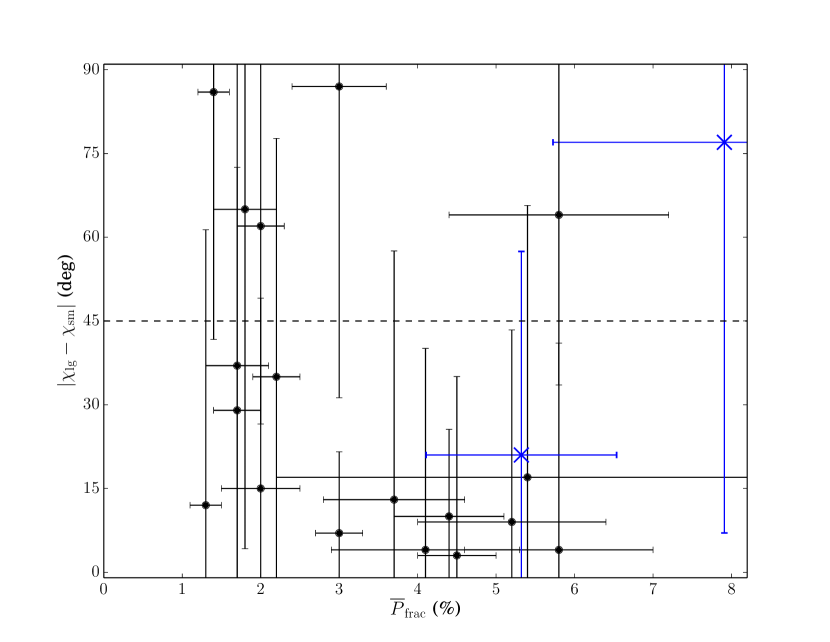
Figure 1.— Large- vs. small-scale B-field orientation $|\chi_{\textrm{lg}}-\chi_{\textrm{sm}}|$ as a function of polarization fraction $\overline{P}_{\textrm{frac}}$. Sources are included if they have (1) B-field detections at both scales, (2) CARMA polarization detections $P_{c}>3.5\,\sigma_{P}$, and (3) distances $d\lesssim 400$ pc. The plotted uncertainty in $|\chi_{\textrm{lg}}-\chi_{\textrm{sm}}|$ is equal to the uncertainties in $\chi_{\textrm{sm}}$ and $\chi_{\textrm{lg}}$ added in quadrature, where those uncertainties reflect the dispersion of the B-field orientations in each source. The fractional polarization $\overline{P}_{\textrm{frac}}=\overline{P}\,/\,\overline{I}$, where $\overline{P}$ and $\overline{I}$ are the unweighted averages of the polarized and total intensities in locations where $P_{c}>3.5\,\sigma_{P}$. Points below the $45\degree$ line exhibit overall alignment between large- and small-scale fields.

While $\sim$ kpc-scale galactic B-fields do not seem to be correlated with smaller-scale B-fields in clouds and cores (e.g., Stephens et al., 2011), Li et al. (2009) did find evidence that B-field orientations are consistent from the $\sim$ 100 pc scales of molecular clouds to the $\sim$ 0.1 pc scales of dense cores. We take the next step by examining the consistency of B-field orientations from the $\sim$ 0.1 pc core to $\sim$ 0.01 pc envelope scales.

In Figure 1 we plot $|\chi_{\textrm{lg}}-\chi_{\textrm{sm}}|$ as a function of the polarization fraction. This plot is limited to sources with (1) B-field detections at both scales, (2) CARMA polarization detections $P_{c}>3.5\,\sigma_{P}$, and (3) distances $d\lesssim 400$ pc.

The most notable feature of the plot is the relative absence of star-forming cores in the upper-right quadrant, i.e., sources that are strongly polarized but have inconsistent large-to-small-scale B-field orientations. With the exception of OMC2-FIR3 and Ser-emb 8, we see that the cores with high CARMA polarization fractions ($\overline{P}_{\textrm{frac}}\geq\,3\%$) have B-field orientations that are consistent from large to small scales. These “high-polarization” sources are L1448 IRS 2 (Figure 6), NGC 1333-IRAS 4A (Figure 12), HH 211 mm (Figure 14), Orion-KL (Figure 19), OMC3-MMS5 and MMS6 (Figure 20), OMC2-FIR3 and 4 (Figure 21), Ser-emb 8 and 8(N) (Figure 26), L1157 (Figure 33), and CB 230 (Figure 34).

In these sources the consistency of the B-fields from large to small scales suggests that the fields have not been twisted by turbulent motions as the material collapses to form the protostellar cores. This is in turn consistent with the sources’ higher fractional polarization, because more ordered B-fields would lead to less averaging of disordered polarization along the LOS. In this subset of sources the B-fields appear to be dynamically important, and may play a role in regulating the infall of material down to $\sim$ 0.01 pc scales.

The remaining “low-polarization” sources ($\overline{P}_{\textrm{frac}}<\,3\%$) are L1448N(B) (Figure 7), NGC 1333-IRAS 2A (Figure 10), SVS 13 (Figure 11), NGC 1333-IRAS 4B (Figure 13), L1551 NE (Figure 16), L1527 (Figure 17), VLA 1623 (Figure 23), and Ser-emb 6 (Figure 27).

Unlike the high-polarization sources, these low-polarization sources may have low ratios of magnetic to turbulent energy, which would result in more twisted small-scale B-fields and thus low CARMA polarization fractions. Note that straight B-fields with a high inclination angle relative to the LOS would also result in low fractional polarization; however, the likelihood of observing B-fields nearly pole-on is low.

Note that we are not asserting that higher polarization is caused directly by stronger B-fields, or that weak polarization occurs because of weak B-fields or poor grain alignment. We simply assume that high and low polarization fractions are caused by B-fields that are less or more twisted, respectively.

We have not yet discussed the more distant sources in our sample, which are all massive star-forming regions (SFRs). Four of these have been observed previously by SCUBA, Hertz, and/or SHARP: W3 Main (Figure 4), W3(OH) (Figure 5), DR21(OH) (Figure 32), and NGC 7538 IRS 1 (Figure 36). It is important to note that we are probing different structures in these objects than we are in the nearby star-forming cores: at the distances to the more distant SFRs, the angular resolution of our CARMA maps corresponds to a spatial resolution of $\sim$ $0.1$ pc. It is evident from our maps that at these scales the B-fields in the SFRs have been twisted, most likely by dynamic processes, as high-mass SFRs are known to be highly turbulent (Elmegreen & Scalo, 2004). This suggests that for massive SFRs the ratio of magnetic to turbulent energy is low at $\sim$ 0.1 pc scales.

V.2. Misalignment of B-fields and bipolar outflows

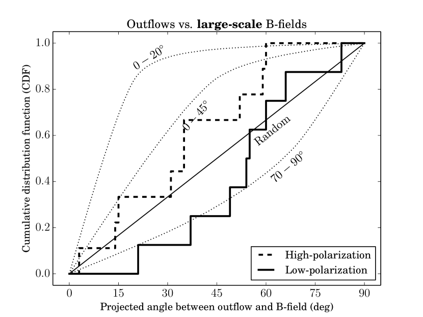
Figure 2.— The thick, stepped curves show the cumulative distribution functions (CDF) of the (projected) angles between the bipolar outflows and the mean large-scale (left) and small-scale (right) B-field orientations in the low-mass protostellar cores listed in Table IV. Sources included in the plot have an asterisk (*) next to their outflow orientation in the table. Large-scale B-fields are from archival CSO and JCMT data, and have $\sim$ $20\arcsec$ resolution; small-scale B-fields are from the CARMA data, and have $\sim$ 2.5$\arcsec$ resolution. The dashed curves include the “high-polarization” sources, and the solid curves include the “low-polarization” sources (see Section V.1 for a discussion of high- vs. low-polarization sources). Sources are included if they have (1) B-field detections at both large and small scales, (2) CARMA polarization detections $P_{c}>3.5\,\sigma_{P}$, (3) distances $d\lesssim 400$ pc, and (4) well defined bipolar outflows. The dotted curves are the CDFs from Monte Carlo simulations where the B-fields and outflows are oriented within $20\degree$, $45\degree$, and 70–90$\degree$ of one another, respectively. The straight line is the CDF for random orientation. The two plots show that outflows appear to be randomly aligned with B-fields; although, in sources with low polarization fractions there is a hint that outflows are preferentially perpendicular to small-scale B-fields, which suggests that in these sources the fields have been wrapped up by envelope rotation (see Section V.2).

We first addressed the question of B-field and outflow misalignment in Hull et al. (2013), where we found that bipolar outflows were randomly aligned with—or perhaps preferentially perpendicular to—the small-scale B-fields in their associated protostellar envelopes. In this paper we use the same sample of nearby ($d\lesssim 400$ pc) low-mass cores with well defined outflows used by Hull et al. (2013), minus IRAS 16293 A, which was not a TADPOL source.

The outflow angles are the same as those used in Hull et al. (2013); the values for $\chi_{\textrm{sm}}$ typically differ by a few degrees because of the inclusion of additional data. Note that we do not include SFRs in this analysis, nor do we include sources with complicated outflow structure such as SVS13 (Figure 11) and OMC2-FIR3/4 (Figure 21). All sources included in Figure 2 have an asterisk (*) next to their outflow orientation in Table IV.

In this paper we extend this analysis to include a comparison of outflow orientations vs. large-scale B-fields. Additionally, for each of these comparisons we split the sources into high- and low-polarization subsamples and plot a separate CDF for each. The heavy dashed and solid curves in Figure 2 correspond to the high- and low-polarization subsamples, respectively.

As discussed in Hull et al. (2013), the B-field and outflow position angles we observe are projected onto the plane of the sky. To determine if the large scatter in position angle differences could be due to projection effects, we compare the results with Monte Carlo simulations where the outflows and B-fields are tightly aligned, somewhat aligned, preferentially perpendicular, or randomly aligned.

For the tightly aligned case, the simulation randomly selects pairs of vectors in three dimensions that are within 20$\degree$ of one another, and then projects the vectors onto the plane of the sky and measures their angular differences. The resulting CDF is shown in Figure 2. In this case projection effects are not as problematic as one might think: to have a projected separation larger than 20$\degree$ the two vectors must point almost along the line of sight.

For the somewhat-aligned and preferentially-perpendicular cases the simulation randomly selects pairs of vectors that are separated by 0–45$\degree$ or 70–90$\degree$, respectively. In these cases projection effects are more important and result in CDFs that are closer to that expected for random alignment, shown by the thin straight line (see Figure 2).

In all four cases in Figure 2 a Kolmogorov–Smirnov (K-S) test rules out the scenario where outflows and B-fields are tightly aligned (the K-S probabilities for all distributions are $<0.002$). This is consistent with the results from Hull et al. (2013), who found that outflows and small-scale B-fields are not tightly aligned.

The K-S test also shows that all of the distributions are consistent with random alignment. However, in low-polarization sources the K-S test gives a probability of only 0.12 that the outflows and small-scale B-fields are randomly aligned, hinting that they may be preferentially perpendicular. (Note that the K-S test does not take into account the dispersions in the B-field orientations reported in Table IV.)

We speculate that the polarization fractions are low in these sources because B-fields have be wrapped up toroidally by envelope rotation. Rotation at $\sim$ 1000 AU scales has been detected in at least two of the sources: see N₂H⁺ observations of CB 230 and CB 244 by Chen et al. (2007) using OVRO (the Owens Valley Radio Observatory). The envelope rotation axes are roughly aligned with the outflow axes in both of these sources.

This result could have important consequences for the formation of circumstellar disks within rotating envelopes, since preferential misalignment of the B-field and the rotation axis should allow disks to form more easily (Hennebelle & Ciardi, 2009; Krasnopolsky et al., 2012; Joos et al., 2012; Li et al., 2013). Objects with misaligned B-fields and rotation axes are less susceptible to the “magnetic braking catastrophe,” where magnetic braking prevents the formation of a rotationally supported Keplerian disk (Allen et al., 2003; Li et al., 2011). Indeed, these models suggest that misalignment may be a necessary condition for the formation of disks (see also Krumholz et al. 2013).

What about the high-polarization population? These could be sources where we do not have the angular resolution to see B-field twisting and instead are seeing a bright sheath of polarized material that has retained the “memory” of the global B-field. Perhaps these are younger sources, or perhaps cores can form with a wide range of B-field strengths (e.g., Vázquez-Semadeni et al., 2011) and some are strong enough to resist twisting.

It is important to emphasize that even if we are seeing wrapped small-scale B-fields in the low-polarization sample, the scales we are probing are $\sim$ 500–1000 AU envelope scales, not $\sim$ 100 AU disk scales. Consequently, the B-fields would have been wrapped up by the envelopes and not by the disks. However, many simulations (e.g., Machida et al., 2006; Myers et al., 2013) expect the B-fields in a protostar to be wrapped up at disk scales, regardless of the larger-scale B-field morphology in the envelope and the core. If this is the case, then with sufficient angular resolution ALMA should see perpendicular B-fields and outflows even in our high-polarization sample.

One possible concern with this analysis is that outflows could disrupt the small-scale B-fields in the protostellar envelopes. And indeed, in a few sources we see hints that the fields are stretched along the direction of the outflow [e.g., NGC-1333 IRAS 2A (Figure 10), HH 211 mm (Figure 14), Ser-emb 6 (Figure 27), and L1157 (Figure 33)]. However, these detections tend to be quite far from the central intensity peak, where the B-field orientation is usually different. This suggests that while outflows may drag B-fields along with them, the outflows do not disrupt the B-fields in the densest parts of the protostellar envelope.

Another concern is that over time outflows could have changed direction, and that deep in the core the outflows and B-fields could actually be aligned. However, many sources show bipolar ejections with consistent position angles over parsec scales. Some examples of such sources from the TADPOL survey include HH 211 mm (Lee et al., 2009), L1448 IRS 2 (Tobin et al., 2007; O’Linger et al., 1999), L1157 (Gueth et al., 1996; Bachiller & Perez Gutierrez, 1997), L1527 (Hogerheijde et al., 1998), and VLA 1623 (Andre et al., 1990).

A source that helps dispel the above concerns is OMC3-MMS6, which has a very small bipolar outflow with a dynamical age of only 100 yr (Takahashi & Ho, 2012), too young to have either perturbed the B-field or changed direction appreciably. As is clear in the maps in Figure 20, the outflow is not aligned with either the large- or the small-scale fields around MMS6, suggesting that the orientation of the disk launching the outflow truly is misaligned with the B-field in the envelope.

V.3. Fractional polarization “hole”

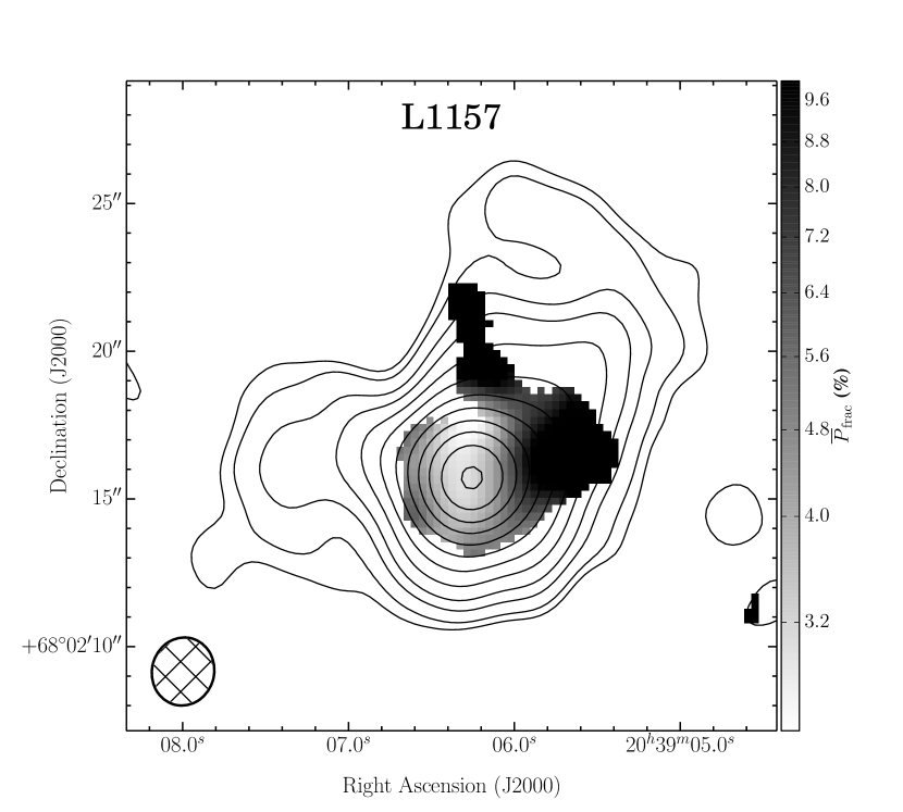
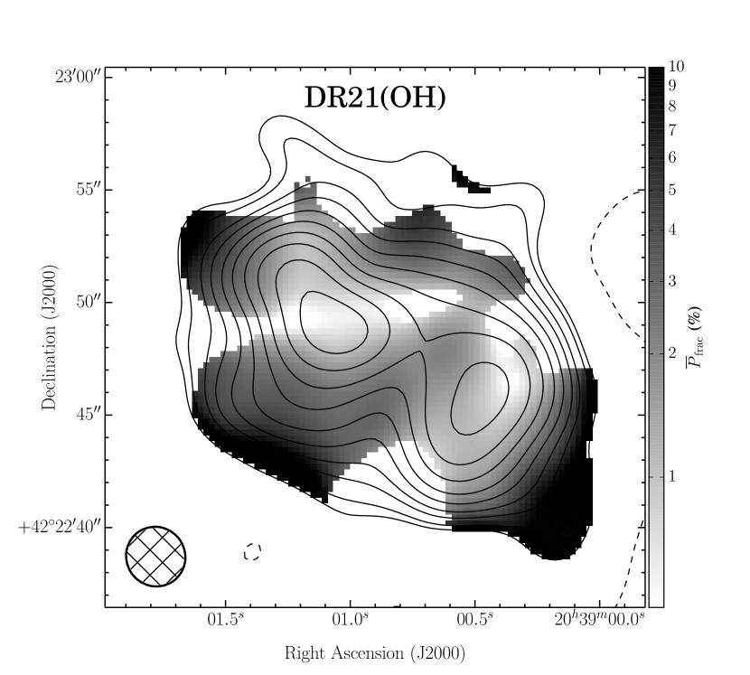
Figure 3.— Sample maps of polarization fraction (grayscale), with dust continuum contours overlaid. The grayscale saturates at 10% in order to emphasize the low polarization fraction near the center of each object; however, the polarization fraction near the edge can be significantly higher. The dust continuum contours in all dust maps are –3, 2, 3, 5, 7, 10, 14, 20, 28, 40, 56, 79, 111, 155, 217 $\times\,\sigma_{I}$ (see Appendix A). Polarization fraction has only been plotted in locations with significant polarization detections (i.e., $P_{c}>3.5\,\sigma_{P}$).

The “polarization hole” effect, where the fractional polarization of protostellar cores drops near their dust emission peaks, is a well known phenomenon that has been seen in many previous observations (e.g., Dotson, 1996; Matthews et al., 2002; Girart et al., 2006; Liu et al., 2013). We see the same effect in all of our maps, for both nearby low-mass sources and distant high-mass sources; this shows that the polarization hole effect is present across many size scales, although the reasons for the effect may be different at different scales. See Figure 3 for sample maps of polarization fraction in L1157 and DR21(OH); these maps show that in both cores and SFRs, the polarization fraction is higher at the edges and lower near the total intensity peaks.

For low resolution maps (e.g., those with $\sim$ 20$\arcsec$ resolution from SCUBA, Hertz, and SHARP), a plausible explanation of the polarization holes was unresolved structure that was averaged across the beam. However, in some of the higher resolution ($\sim$ 2.5$\arcsec$ resolution) maps presented here and in previous interferometric observations, these twisted plane-of-sky B-field morphologies have been resolved, and yet the drop in fractional polarization persists.

There are multiple possible explanations. First, except for a very few lines of sight through the densest parts of protostellar disks, millimeter-wavelength thermal dust emission is optically thin, and thus we are integrating along the LOS. If the B-field orientation is not consistent along the LOS (due to turbulence or rotation, for example), averaging will result in reduced fractional polarization. Second, there could still be unresolved B-field structure in the plane of the sky at scales smaller than the $\sim$ 2.5$\arcsec$ resolution of the CARMA data (e.g., Rao et al., 1998). And third, grains at the centers of cores could be poorly aligned because grain alignment is less efficient in regions with high extinction, or because collisions knock grains out of alignment at higher densities. Simulations of polarized emission from turbulent cores that include the above effects show the polarization hole (e.g., Padoan et al., 2001; Lazarian, 2005; Bethell et al., 2007; Pelkonen et al., 2009).

VI. SUMMARY

We have presented polarization maps of low-mass star-forming cores and high-mass star-forming regions from the TADPOL survey. Using source-averaged B-field orientations and polarization fractions, we have studied the statistical properties of the ensemble of sources and have come to the following key conclusions:

1. Sources with high CARMA polarization fractions also have consistent B-field orientations on large ($\sim$ 20$\arcsec$) and small ($\sim$ 2.5$\arcsec$) scales. We interpret this to mean that in at least some cases B-fields play a role in regulating the infall of material all the way down to the $\sim$ 1000 AU scales of protostellar envelopes.

2. Outflows appear to be randomly aligned with B-fields; although, in sources with low polarization fractions there is a hint that outflows are preferentially perpendicular to small-scale B-fields, which suggests that in these sources the fields have been wrapped up by envelope rotation.

3. Finally, even at $\sim$ 2.5$\arcsec$ resolution we see the so-called “polarization hole” effect, where the fractional polarization drops significantly near the total intensity peak.

As the largest survey of low-mass protostellar cores to date, the TADPOL project sets the stage for observations with ALMA. ALMA’s unprecedented sensitivity will allow us to answer the question of what happens to magnetic fields in very young Class 0 protostars between the $\sim$ 1000 AU scales we probe in this work and the $\sim$ 100 AU scales of the circumstellar disks. The addition of ALMA data to the TADPOL sample will also enable more robust statistical analyses of the types done in both this work and in Hull et al. (2013), and will allow us to see trends in B-field morphology with source mass, age, environment, multiplicity, envelope rotation, outflow velocity, and B-field strength.

Appendix A APPENDIX A: SOURCE MAPS

All maps from the TADPOL survey are publicly available as FITS images and machine readable tables. For each figure below we include maps of Stokes $I$, $Q$, and $U$; bias-corrected polarization intensity $P_{c}$; polarization fraction $P_{\textrm{frac}}=P_{c}/I$; and inferred B-field orientation $\chi_{\textrm{sm}}$. Additionally, we include FITS cubes of total intensity (Stokes $I$) spectral-line data, as well as machine readable tables listing the RA, DEC, $I$, $P_{c}$, $P_{\textrm{frac}}$, $\chi_{\textrm{sm}}$, and associated uncertainties of each line segment plotted in the figures. These files are available in a .tar.gz package available via the link in the figure caption.

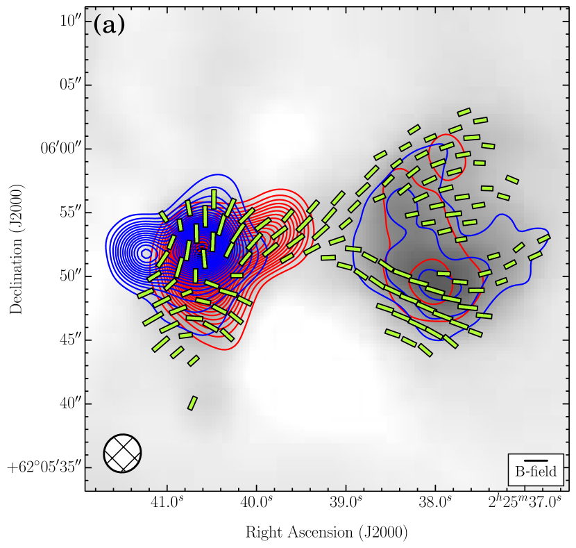
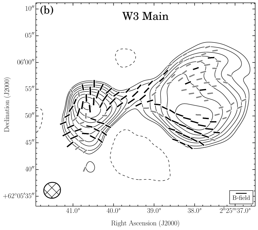
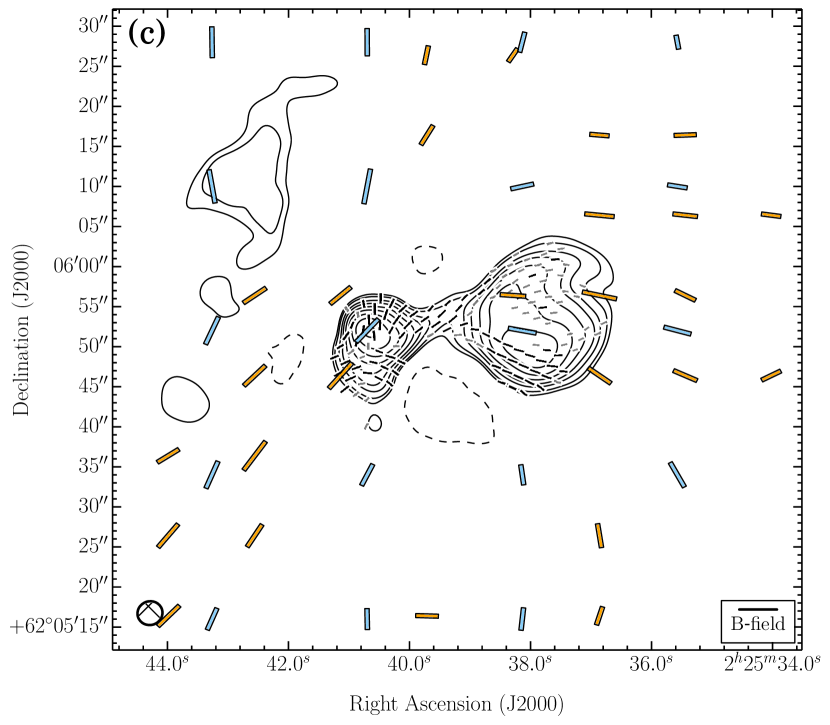
Figure 4.— Maps of W3 Main. The line segments show the inferred magnetic field orientations; they have been rotated by 90$\degree$ relative to the polarization orientations. Segments are plotted twice per synthesized beam (resolution element) in locations where $I>2\,\sigma_{I}$ and $P_{c}>2\,\sigma_{P}$, where $I$ is the total intensity of the dust emission, $P_{c}$ is the bias-corrected polarized intensity, and $\sigma_{I}$ and $\sigma_{P}$ are the rms noise values in the total and polarized intensity maps, respectively. (a) The segment lengths are proportional to the square root of polarized intensity, not fractional polarization. The grayscale is proportional to the total intensity (Stokes $I$) dust emission. The blue and red contours are the blue- and redshifted spectral line wings. The outflow orientation is indicated by a gray line for sources with outflows listed in Table IV. The velocity ranges of the CO($J=2\rightarrow 1$) emission in this map are –2.3 to –10.8 km s^-1 (redshifted) and –67.9 to –80.6 km s^-1 (blueshifted). The contour levels in all spectral line maps are 4, 8, 12, 16 and  20, 25, 30 … 190, 195, 200 $\times\,\sigma_{\textrm{SL}}$, where $\sigma_{\textrm{SL}}$ is the rms noise measured in the spectral line moment maps. In this map, $\sigma_{\textrm{SL}}=0.50$ K km s^-1. (b) Line segments are black where $P_{c}>3.5\,\sigma_{P}$ and gray where $2\,\sigma_{P}<P_{c}<3.5\,\sigma_{P}$. The grid on which the line segments are plotted is centered on the polarization intensity peak $P_{\textrm{c,pk}}$, which is not necessarily spatially coincident with the total intensity peak $I_{\textrm{pk}}$. The ellipses show the synthesized beams. The dust continuum contours in all dust maps are –3, 2, 3, 5, 7, 10, 14, 20, 28, 40, 56, 79, 111, 155, 217 $\times\,\sigma_{I}$. In this map, $\sigma_{I}=8.8$ mJy bm^-1. (c) Same dust contours and B-field orientations as in (b), with data from three submillimeter polarimeters overlaid: SCUBA (in orange, from Matthews et al. 2009), Hertz (in light blue, from Dotson et al. 2010), and SHARP (in purple, from Attard et al. 2009; Davidson et al. 2011; Chapman et al. 2013). For SCUBA, Hertz, and SHARP data the segment lengths are proportional to the square root of the polarized intensity.

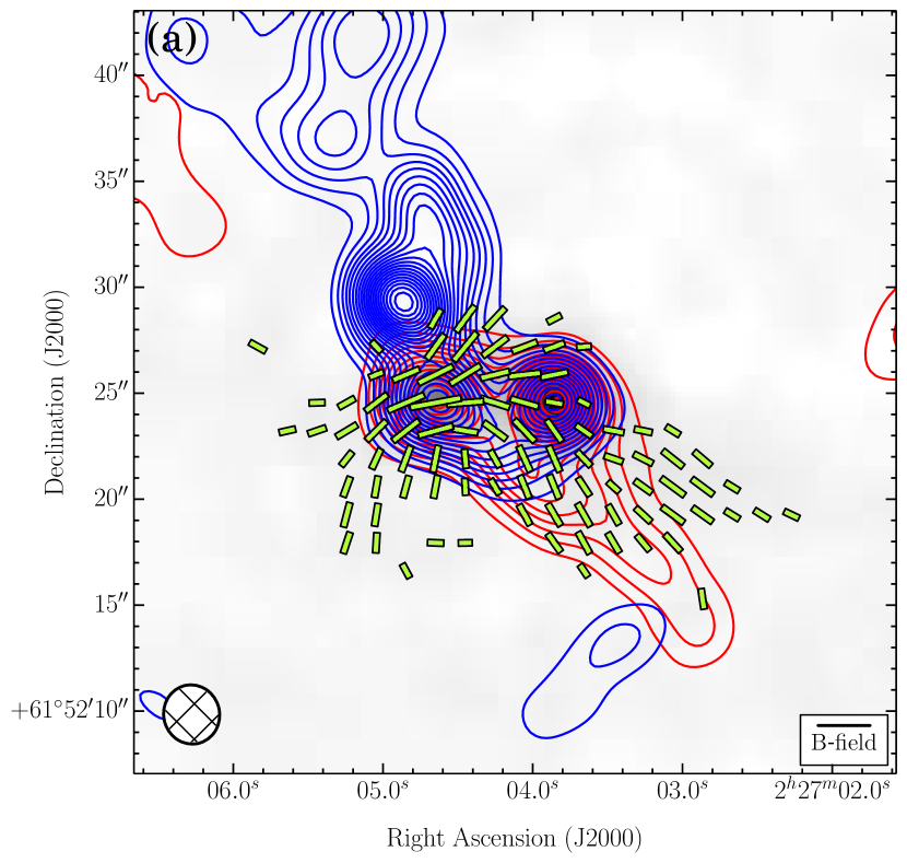
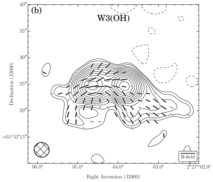
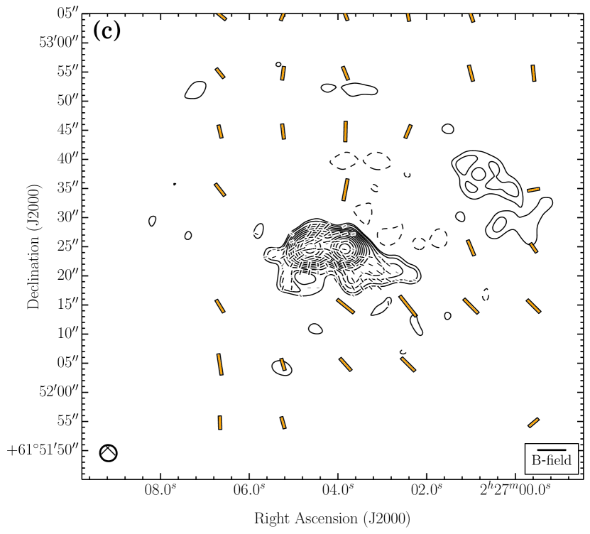
Figure 5.— W3(OH). Same as Figure 4. (a) The velocity ranges of the CO($J=2\rightarrow 1$) line wing emission are –13.4 to –34.5 km s^-1 (redshifted) and –57.8 to –72.6 km s^-1 (blueshifted). $\sigma_{\textrm{SL}}=1.97$ K km s^-1. (b) $\sigma_{I}=14.4$ mJy bm^-1.

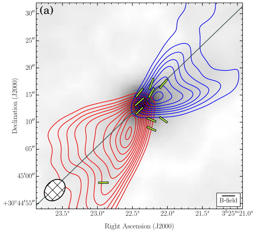
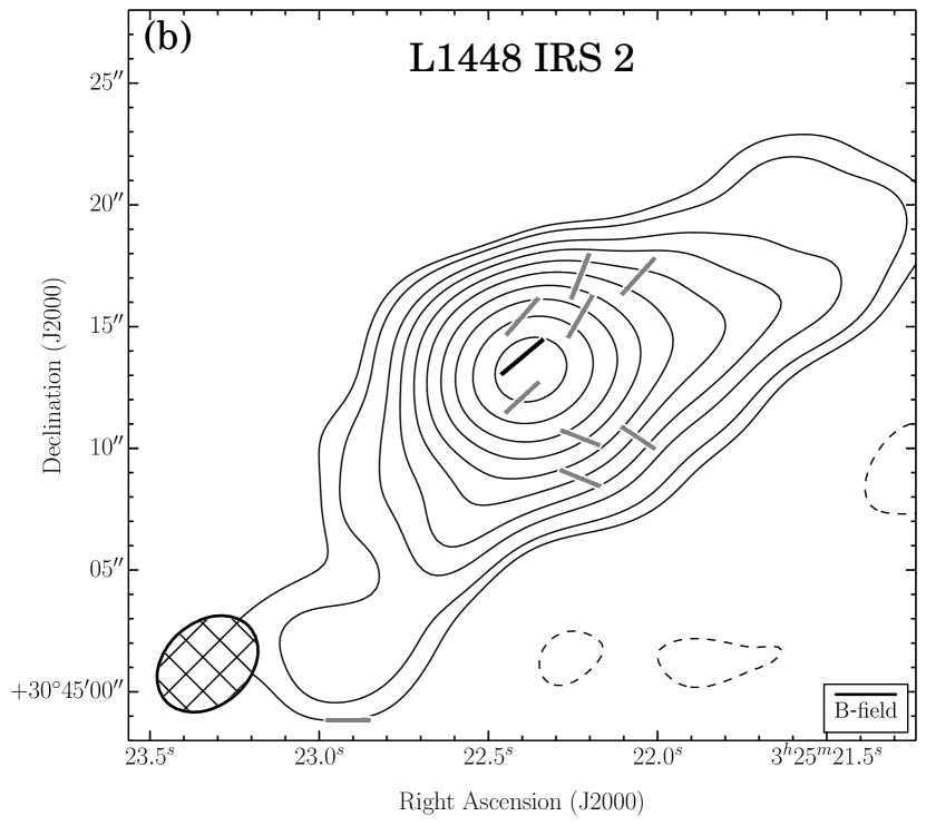
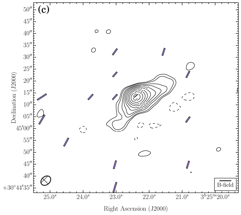
Figure 6.— L1448 IRS 2. Same as Figure 4. (a) The velocity ranges of the CO($J=2\rightarrow 1$) line wing emission are 18.0 to 7.5 km s^-1 (redshifted) and 1.1 to –6.3 km s^-1 (blueshifted). $\sigma_{\textrm{SL}}=1.39$ K km s^-1. (b) $\sigma_{I}=2.0$ mJy bm^-1.

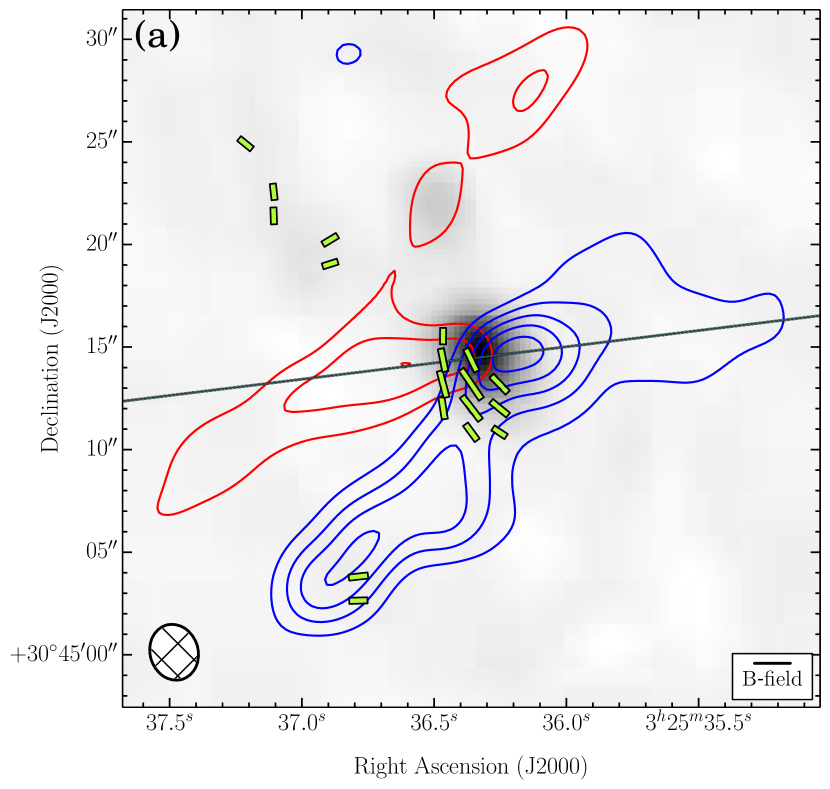
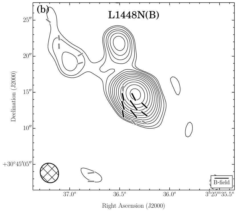
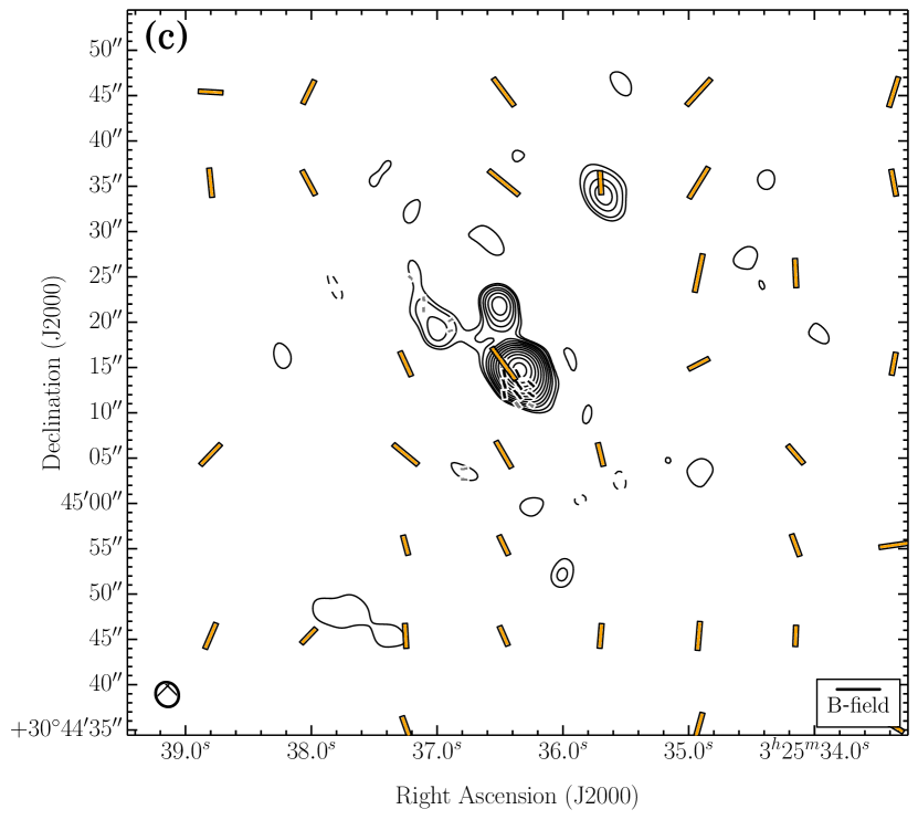
Figure 7.— L1448N(B). Same as Figure 4. (a) The velocity ranges of the CO($J=2\rightarrow 1$) line wing emission are 25.4 to 11.6 km s^-1 (redshifted) and –0.0 to –11.7 km s^-1 (blueshifted). $\sigma_{\textrm{SL}}=4.33$ K km s^-1. (b) $\sigma_{I}=4.5$ mJy bm^-1.

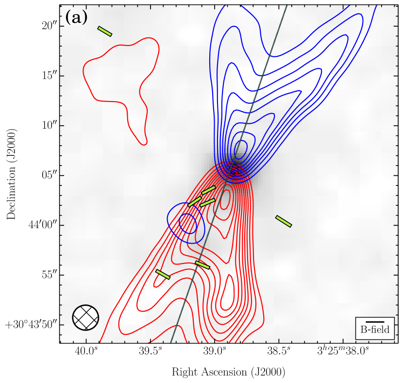
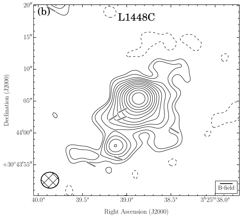
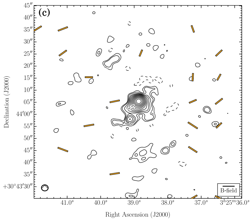
Figure 8.— L1448C. Same as Figure 4. (a) The velocity ranges of the CO($J=2\rightarrow 1$) line wing emission are 15.0 to 7.6 km s^-1 (redshifted) and 1.3 to –12.5 km s^-1 (blueshifted). $\sigma_{\textrm{SL}}=3.01$ K km s^-1. (b) $\sigma_{I}=1.2$ mJy bm^-1.

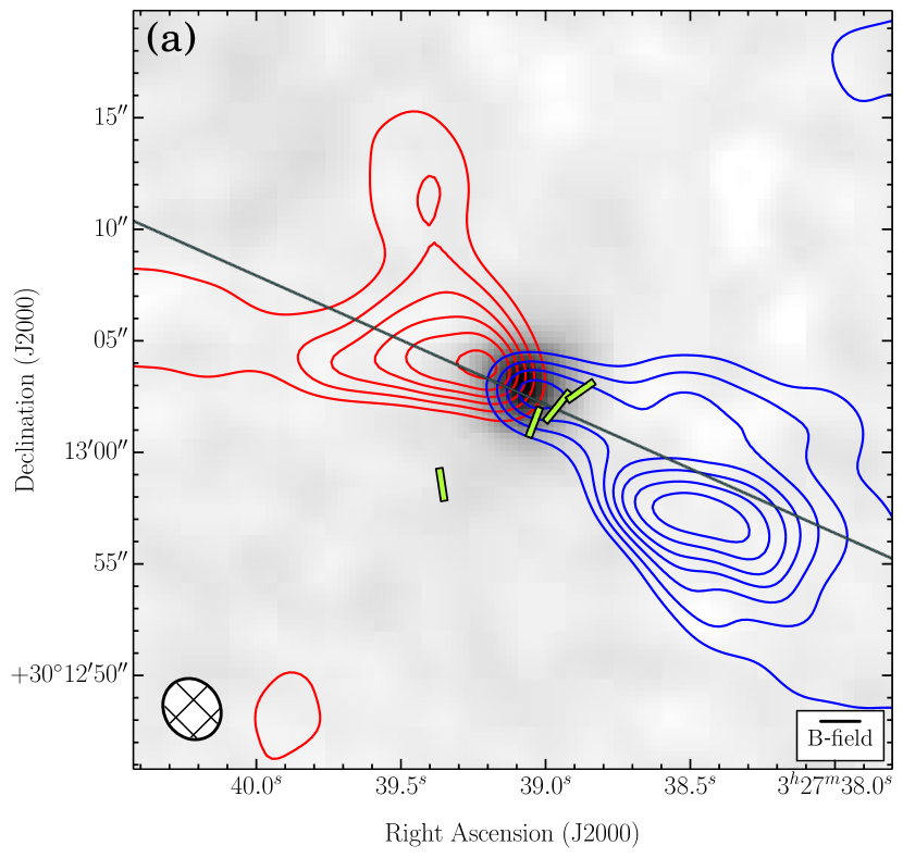
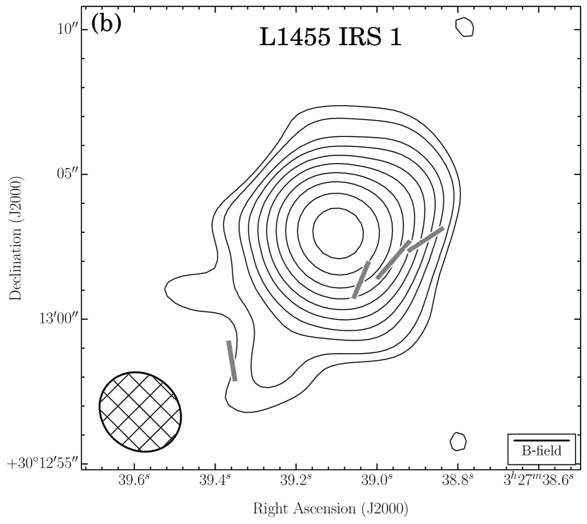
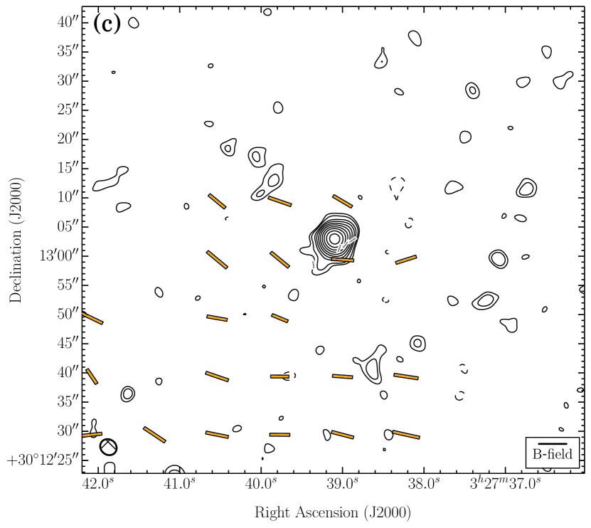
Figure 9.— L1455 IRS 1. Same as Figure 4. (a) The velocity ranges of the CO($J=2\rightarrow 1$) line wing emission are 15.7 to 7.2 km s^-1 (redshifted) and 3.0 to –2.3 km s^-1 (blueshifted). $\sigma_{\textrm{SL}}=1.26$ K km s^-1. (b) $\sigma_{I}=0.6$ mJy bm^-1.

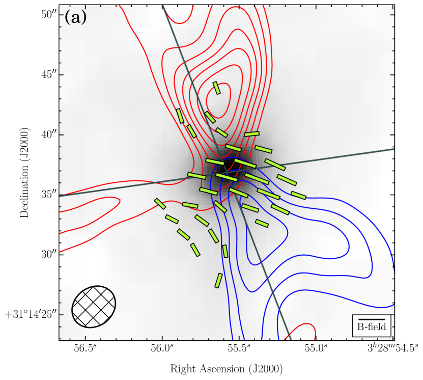
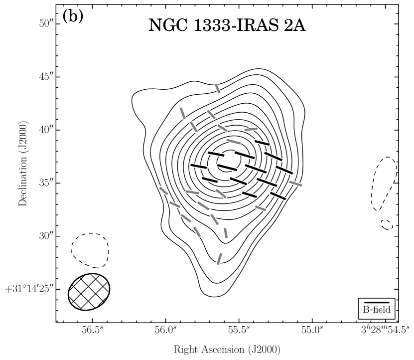
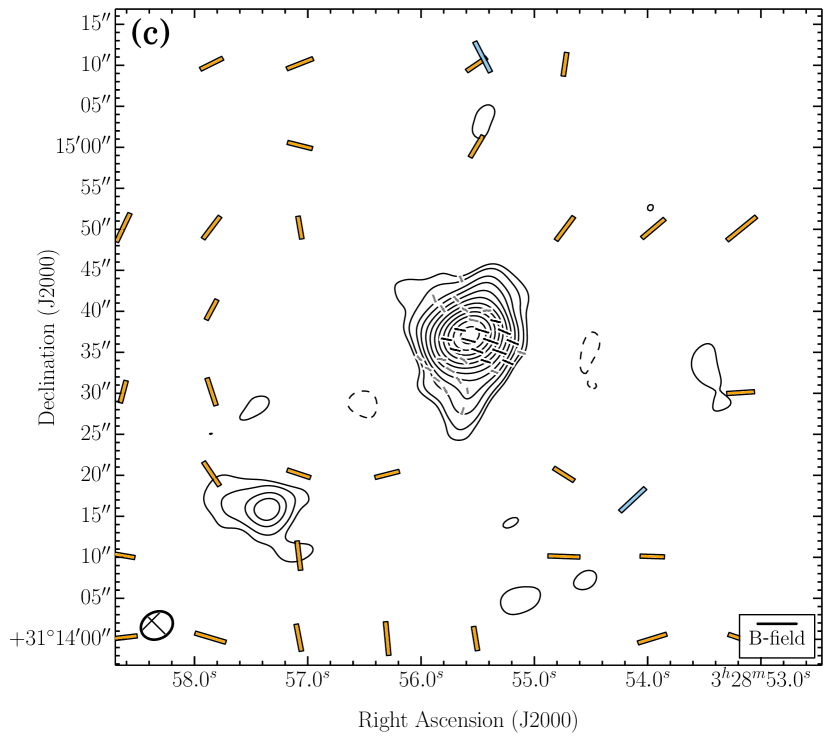
Figure 10.— NGC 1333-IRAS 2A. Same as Figure 4. (a) The velocity ranges of the CO($J=2\rightarrow 1$) line wing emission are 27.0 to 10.1 km s^-1 (redshifted) and 2.6 to –5.8 km s^-1 (blueshifted). $\sigma_{\textrm{SL}}=2.07$ K km s^-1. (b) $\sigma_{I}=2.4$ mJy bm^-1.

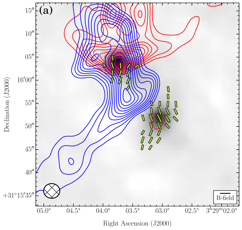
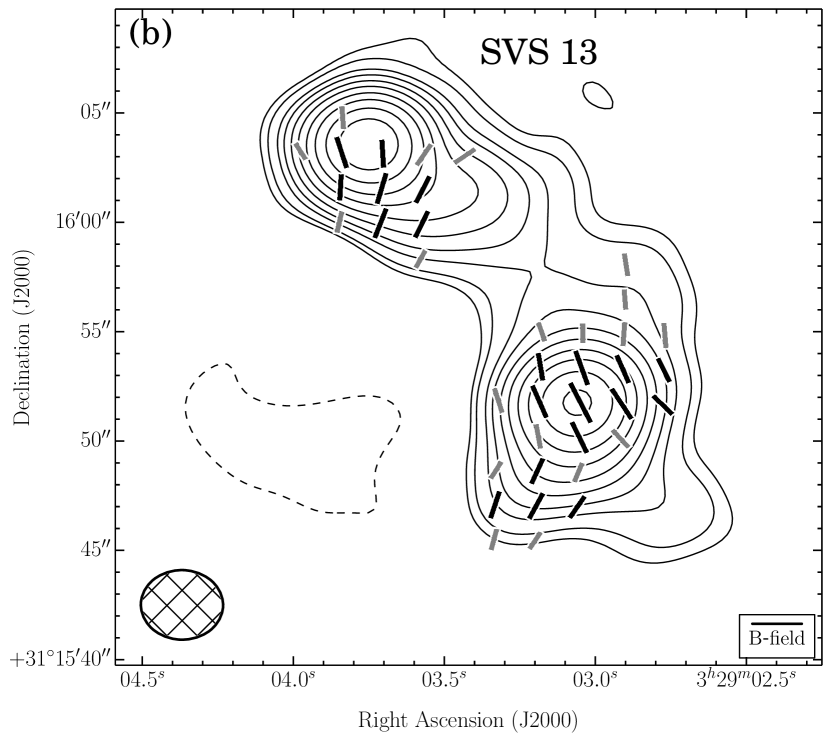
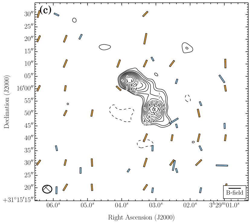
Figure 11.— SVS 13. Same as Figure 4. (a) The velocity ranges of the CO($J=2\rightarrow 1$) line wing emission are 27.0 to 19.6 km s^-1 (redshifted) and –6.9 to –12.2 km s^-1 (blueshifted). $\sigma_{\textrm{SL}}=0.59$ K km s^-1. (b) $\sigma_{I}=3.6$ mJy bm^-1.

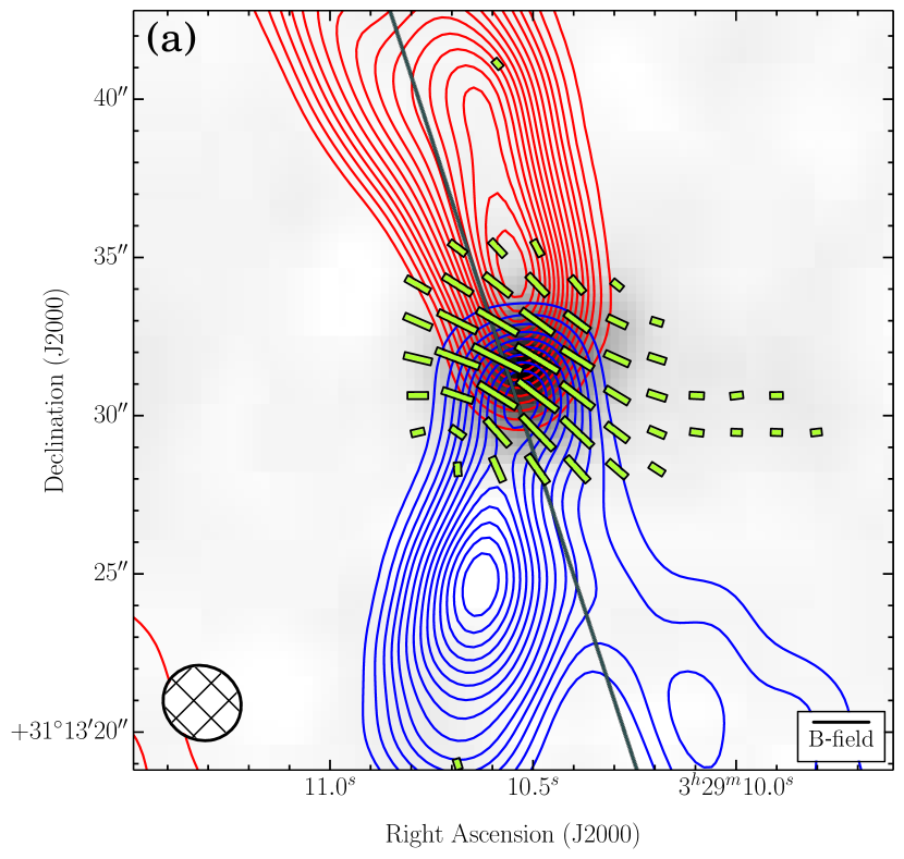
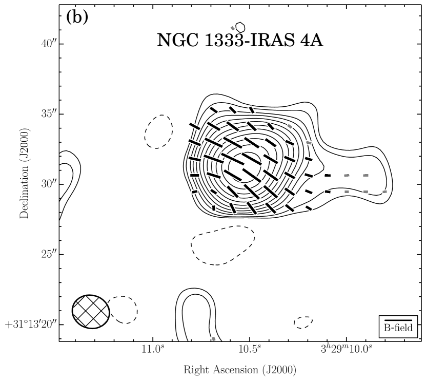
Figure 12.— NGC 1333-IRAS 4A. Same as Figure 4. (a) The velocity ranges of the CO($J=2\rightarrow 1$) line wing emission are 11.2 to 3.8 km s^-1 (redshifted) and –4.6 to –14.2 km s^-1 (blueshifted). $\sigma_{\textrm{SL}}=2.41$ K km s^-1. (b) $\sigma_{I}=10.9$ mJy bm^-1.

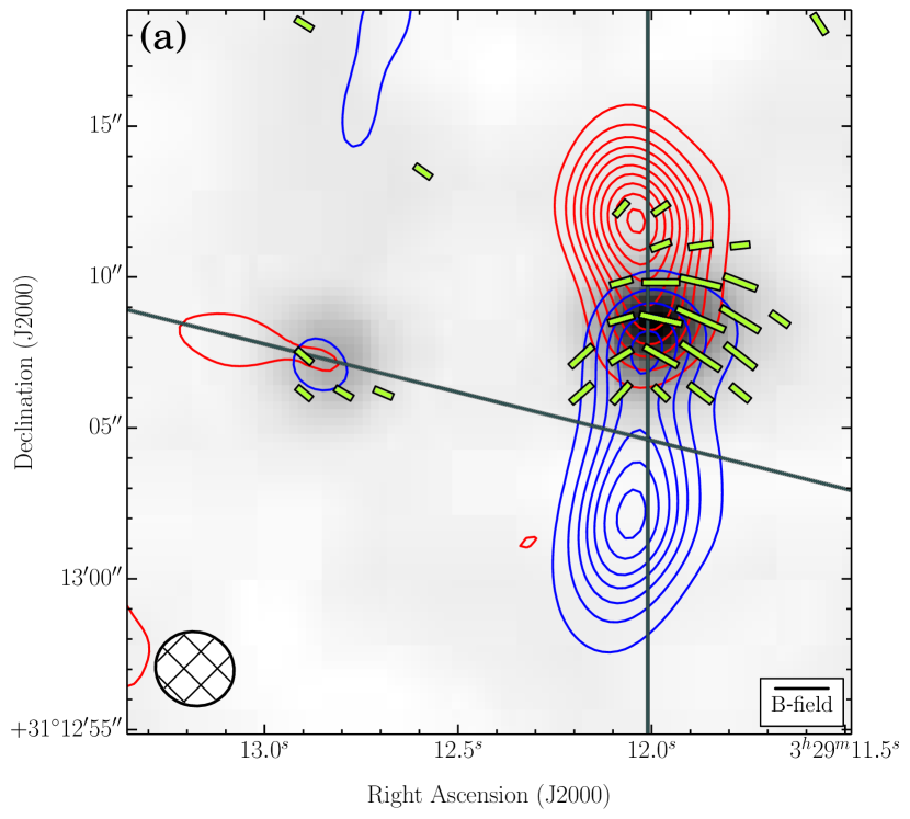
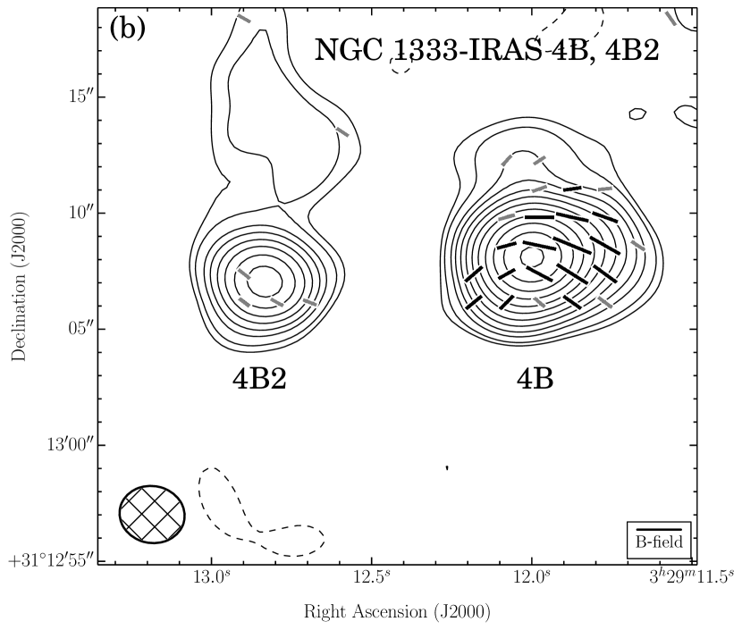
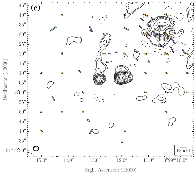
Figure 13.— NGC 1333-IRAS 4B and 4B2. Same as Figure 4. (a) The velocity ranges of the CO($J=2\rightarrow 1$) line wing emission are 22.5 to 9.8 km s^-1 (redshifted) and 3.4 to –12.5 km s^-1 (blueshifted). $\sigma_{\textrm{SL}}=3.12$ K km s^-1. (b) $\sigma_{I}=7.3$ mJy bm^-1.

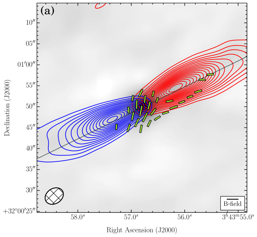
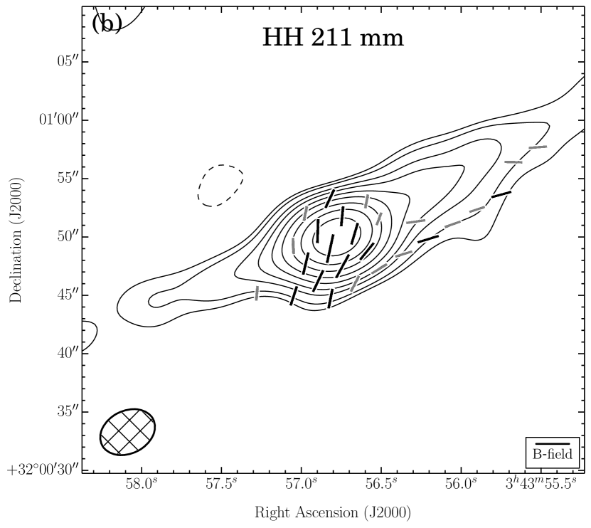
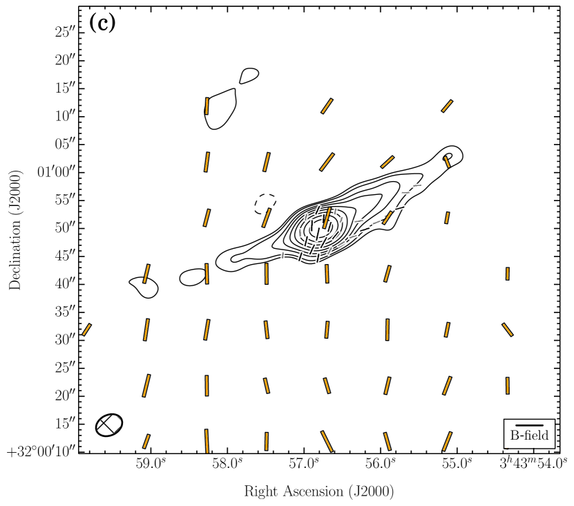
Figure 14.— HH 211 mm. Same as Figure 4. (a) The velocity ranges of the CO($J=2\rightarrow 1$) line wing emission are 29.6 to 12.6 km s^-1 (redshifted) and 6.3 to –3.2 km s^-1 (blueshifted). $\sigma_{\textrm{SL}}=1.03$ K km s^-1. (b) $\sigma_{I}=3.5$ mJy bm^-1.

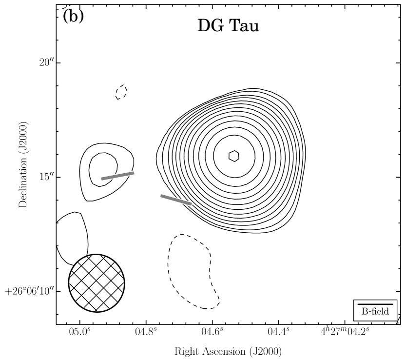
Figure 15.— DG Tau. Same as Figure 4. (a) The velocity ranges of the CO($J=2\rightarrow 1$) line wing emission are 13.3 to 8.0 km s^-1 (redshifted) and 4.9 to 0.6 km s^-1 (blueshifted). $\sigma_{\textrm{SL}}=0.85$ K km s^-1. (b) $\sigma_{I}=1.9$ mJy bm^-1. There is no (c) plot because there were no SCUBA, SHARP, or Hertz data to overlay.

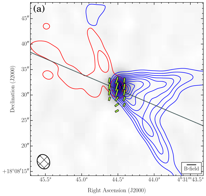
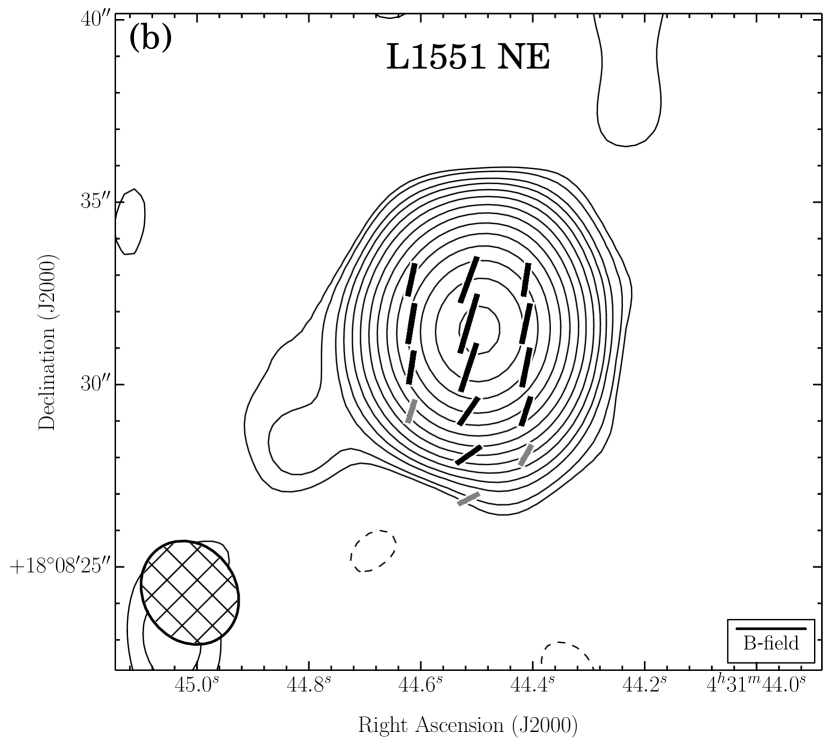
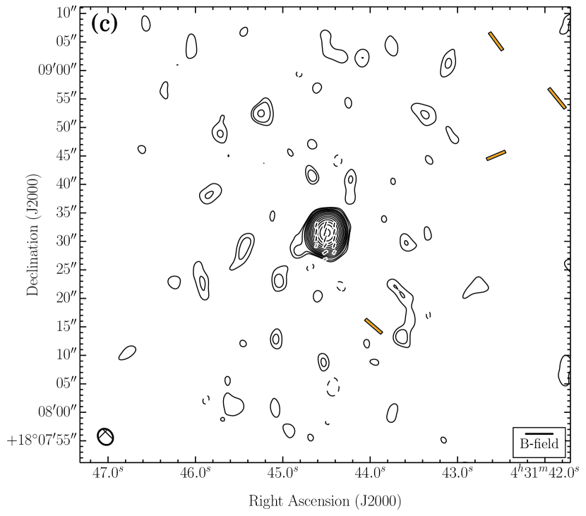
Figure 16.— L1551 NE. Same as Figure 4. (a) The velocity ranges of the CO($J=2\rightarrow 1$) line wing emission are 22.5 to 15.0 km s^-1 (redshifted) and 3.4 to –1.9 km s^-1 (blueshifted). $\sigma_{\textrm{SL}}=0.75$ K km s^-1. (b) $\sigma_{I}=1.8$ mJy bm^-1.

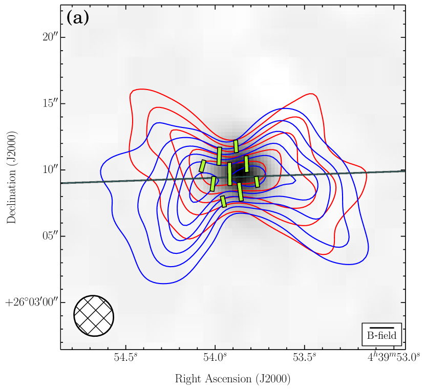
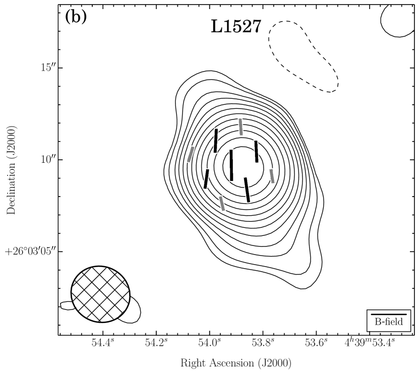
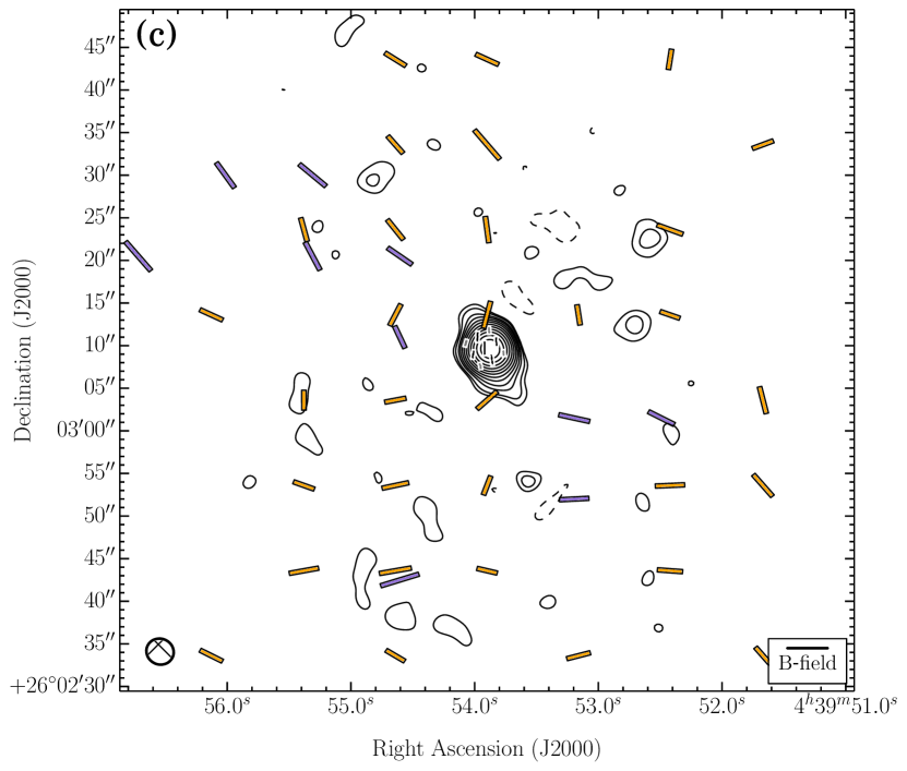
Figure 17.— L1527. Same as Figure 4. (a) The velocity ranges of the CO($J=2\rightarrow 1$) line wing emission are 12.9 to 9.7 km s^-1 (redshifted) and 2.3 to –0.9 km s^-1 (blueshifted). $\sigma_{\textrm{SL}}=0.32$ K km s^-1. (b) $\sigma_{I}=1.0$ mJy bm^-1.

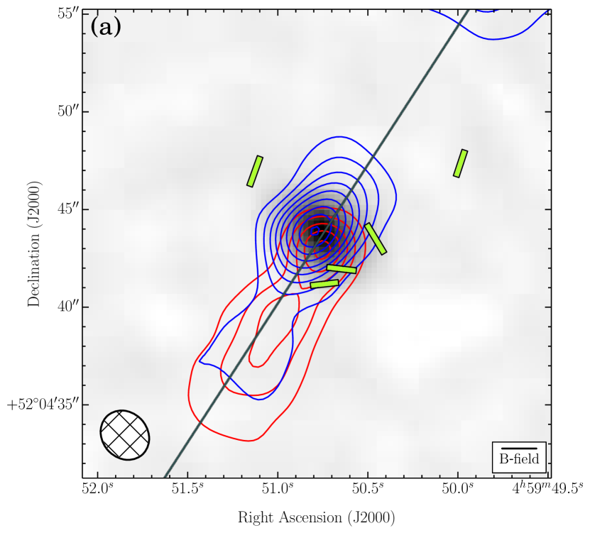
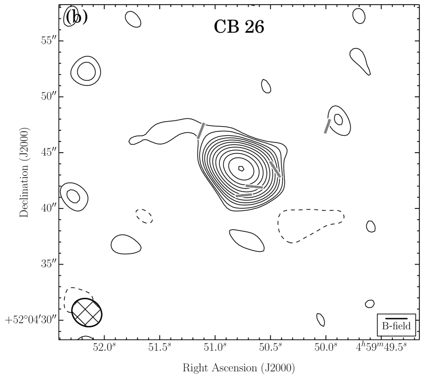
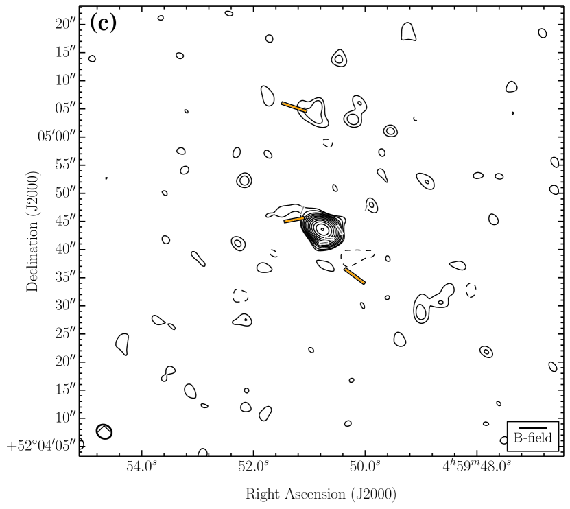
Figure 18.— CB 26. Same as Figure 4. (a) The velocity ranges of the CO($J=2\rightarrow 1$) line wing emission are 11.4 to 8.3 km s^-1 (redshifted) and 4.0 to –0.2 km s^-1 (blueshifted). $\sigma_{\textrm{SL}}=0.46$ K km s^-1. (b) $\sigma_{I}=0.7$ mJy bm^-1.

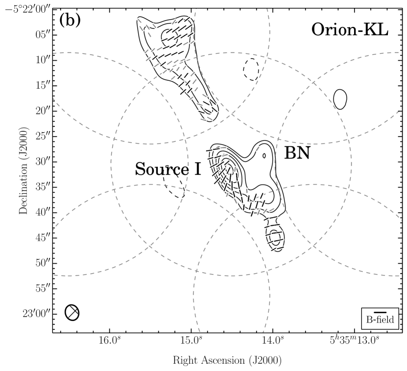
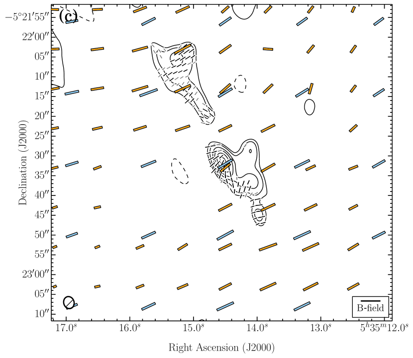
Figure 19.— Orion-KL. Same as above. (b) $\sigma_{I}=211.0$ mJy bm^-1. The full-width-half-max (FWHM) of the 7 mosaic pointings are plotted as gray, dotted circles. Their diameters ($\sim$ 44$\arcsec$) reflect the average primary beam size of the 6 and 10 m telescopes. There is no (a) plot because there were no spectral-line data to plot.

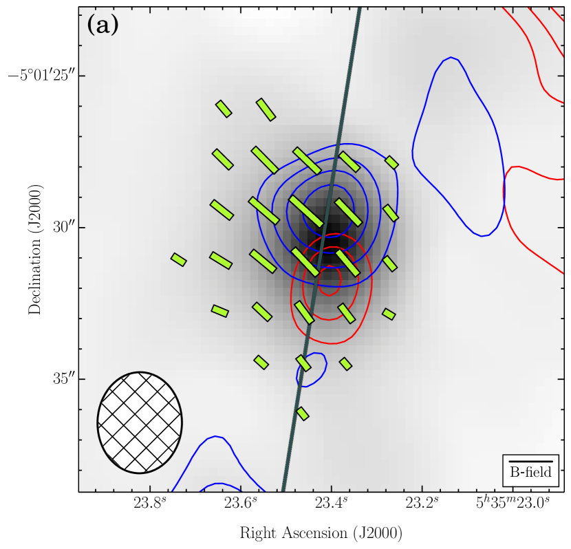
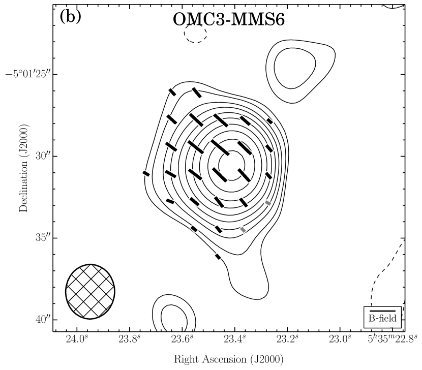
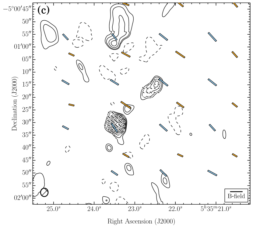
Figure 20.— OMC3-MMS5 and MMS6. Same as Figure 4. (a) The velocity ranges of the CO($J=2\rightarrow 1$) line wing emission are 20.7 to 16.5 km s^-1 (redshifted) and 5.9 to 3.8 km s^-1 (blueshifted). $\sigma_{\textrm{SL}}=0.24$ K km s^-1. (b) $\sigma_{I}=15.0$ mJy bm^-1.

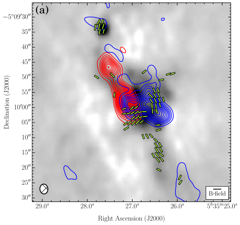
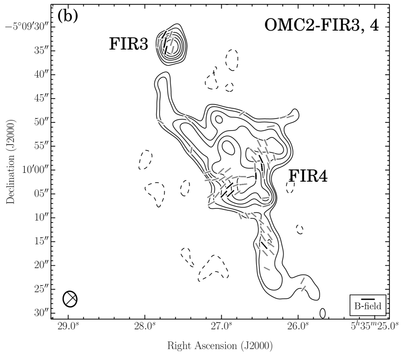
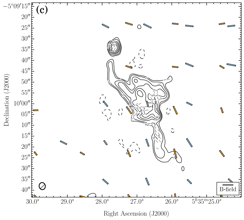
Figure 21.— OMC2-FIR3 and 4. Same as Figure 4. (a) The velocity ranges of the CO($J=2\rightarrow 1$) line wing emission are 33.1 to 20.4 km s^-1 (redshifted) and 1.4 to –11.3 km s^-1 (blueshifted). $\sigma_{\textrm{SL}}=1.35$ K km s^-1. (b) $\sigma_{I}=3.5$ mJy bm^-1.

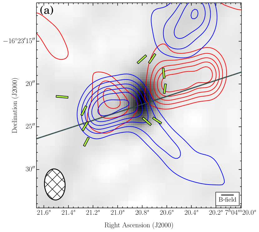
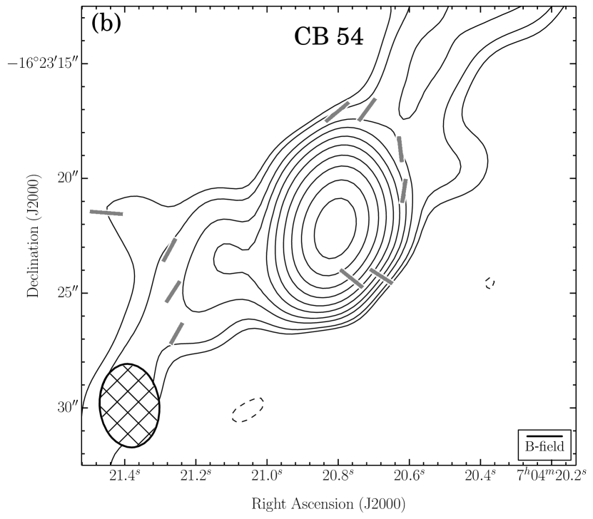
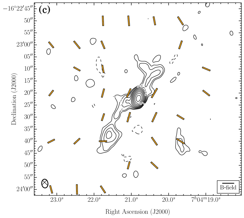
Figure 22.— CB 54. Same as Figure 4. (a) The velocity ranges of the CO($J=2\rightarrow 1$) line wing emission are 28.0 to 23.8 km s^-1 (redshifted) and 14.3 to 9.0 km s^-1 (blueshifted). $\sigma_{\textrm{SL}}=1.28$ K km s^-1. (b) $\sigma_{I}=1.3$ mJy bm^-1.

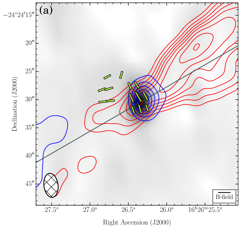
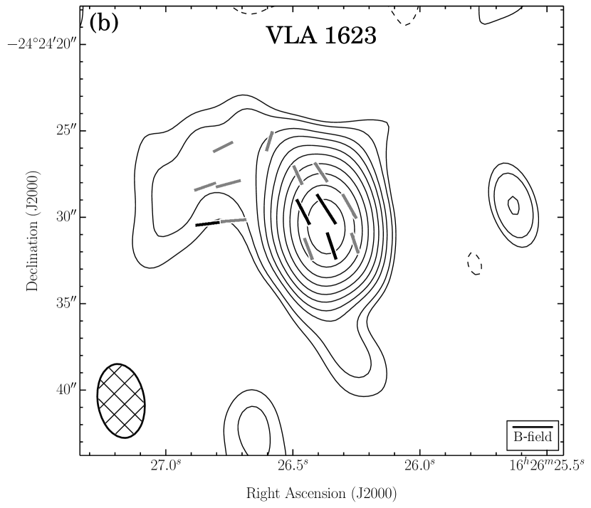
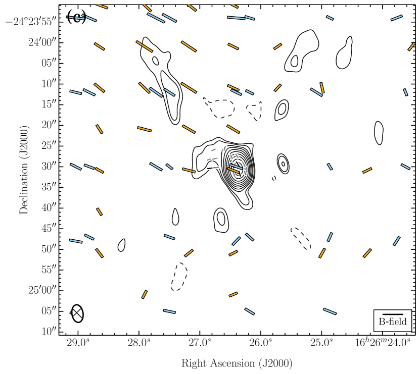
Figure 23.— VLA 1623. Same as Figure 4. (a) The velocity ranges of the CO($J=2\rightarrow 1$) line wing emission are 15.2 to 5.7 km s^-1 (redshifted) and –1.7 to –9.1 km s^-1 (blueshifted). $\sigma_{\textrm{SL}}=0.98$ K km s^-1. (b) $\sigma_{I}=3.8$ mJy bm^-1.

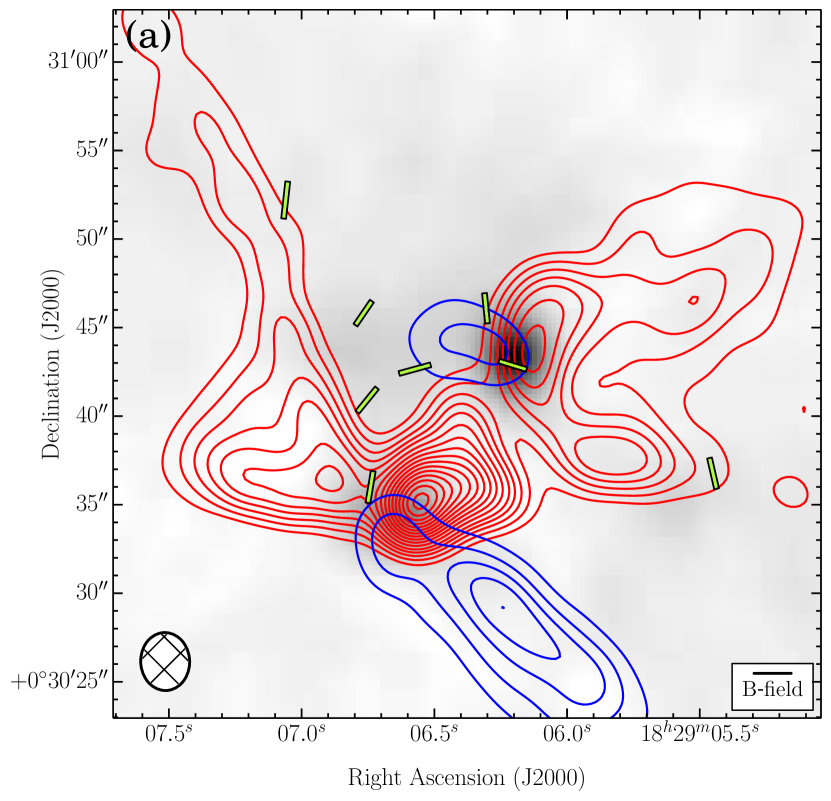
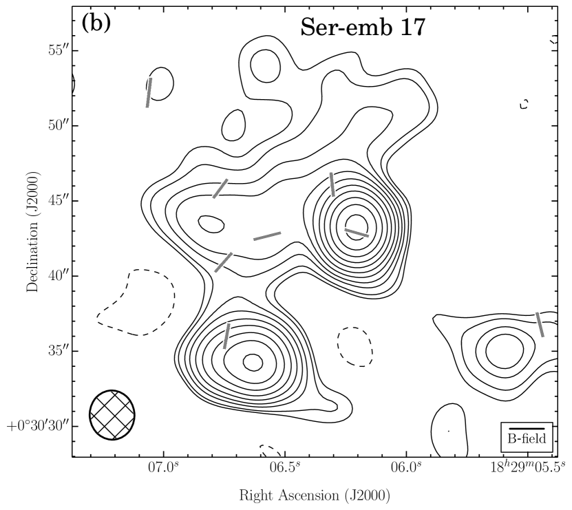
Figure 24.— Ser-emb 17. Same as Figure 4. (a) The velocity ranges of the CO($J=2\rightarrow 1$) line wing emission are 15.4 to 12.2 km s^-1 (redshifted) and –2.6 to –11.1 km s^-1 (blueshifted). $\sigma_{\textrm{SL}}=1.13$ K km s^-1. (b) $\sigma_{I}=1.7$ mJy bm^-1. There is no (c) plot because there were no SCUBA, SHARP, or Hertz data to overlay.

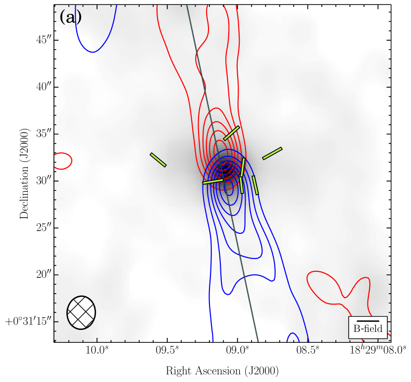
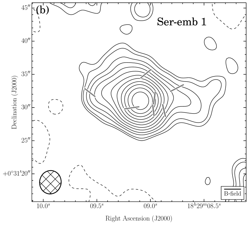
Figure 25.— Ser-emb 1. Same as Figure 4. (a) The velocity ranges of the CO($J=2\rightarrow 1$) line wing emission are 27.0 to 13.3 km s^-1 (redshifted) and 3.8 to –11.1 km s^-1 (blueshifted). $\sigma_{\textrm{SL}}=2.16$ K km s^-1. (b) $\sigma_{I}=1.4$ mJy bm^-1. There is no (c) plot because there were no SCUBA, SHARP, or Hertz data to overlay.

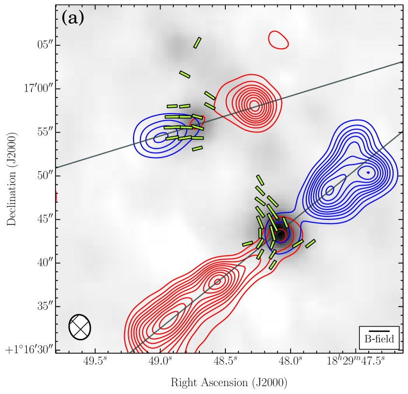
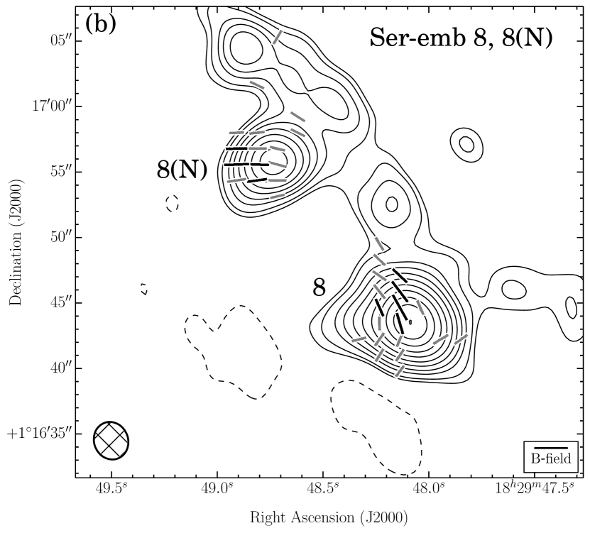
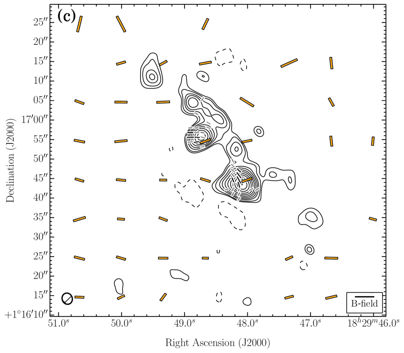
Figure 26.— Ser-emb 8 and 8(N). Same as Figure 4. (a) The velocity ranges of the SiO($J=5\rightarrow 4$) line wing emission are 23.7 to 10.2 km s^-1 (redshifted) and 4.6 to –6.6 km s^-1 (blueshifted). $\sigma_{\textrm{SL}}=0.62$ K km s^-1. (b) $\sigma_{I}=2.1$ mJy bm^-1. Note: in Hull et al. (2013), the colors of the red- and blueshifted outflow lobes were accidentally reversed.

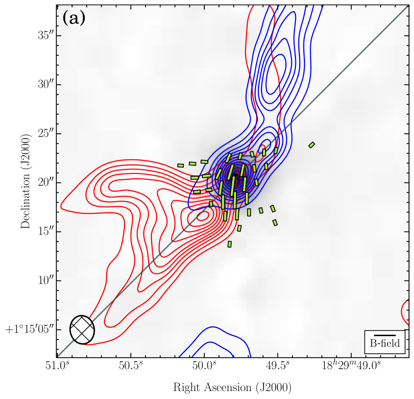
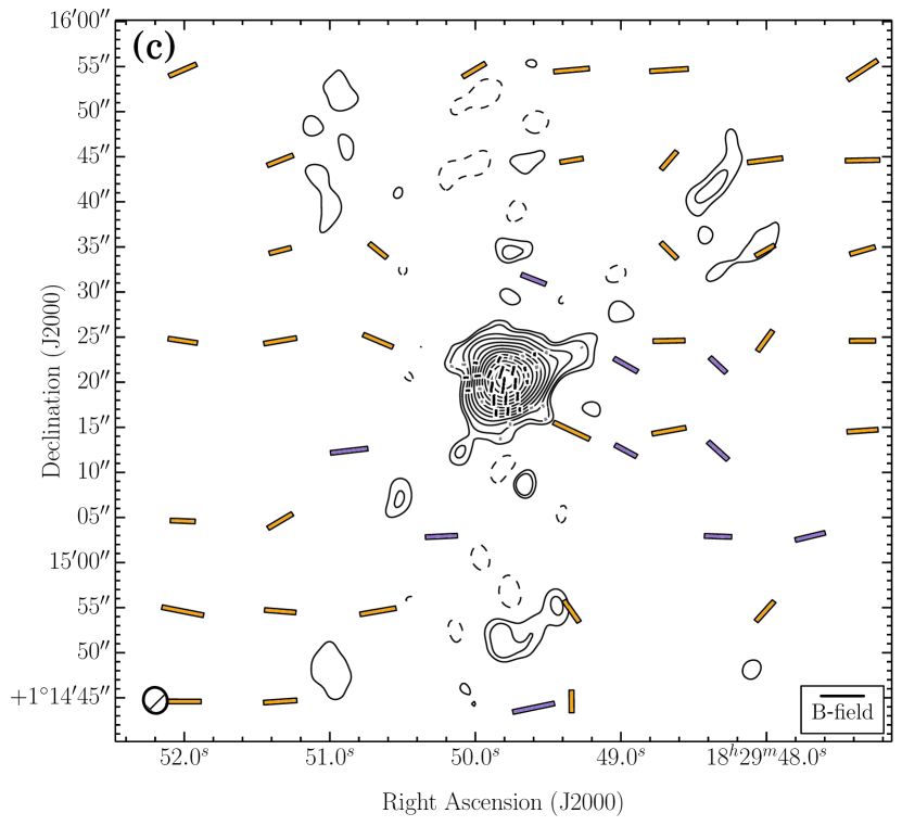
Figure 27.— Ser-emb 6. Same as Figure 4. (a) The velocity ranges of the CO($J=2\rightarrow 1$) line wing emission are 23.9 to 16.4 km s^-1 (redshifted) and 1.6 to –11.1 km s^-1 (blueshifted). $\sigma_{\textrm{SL}}=2.35$ K km s^-1. (b) $\sigma_{I}=6.2$ mJy bm^-1.

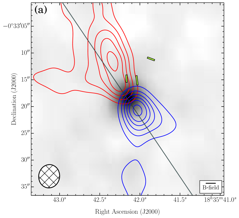
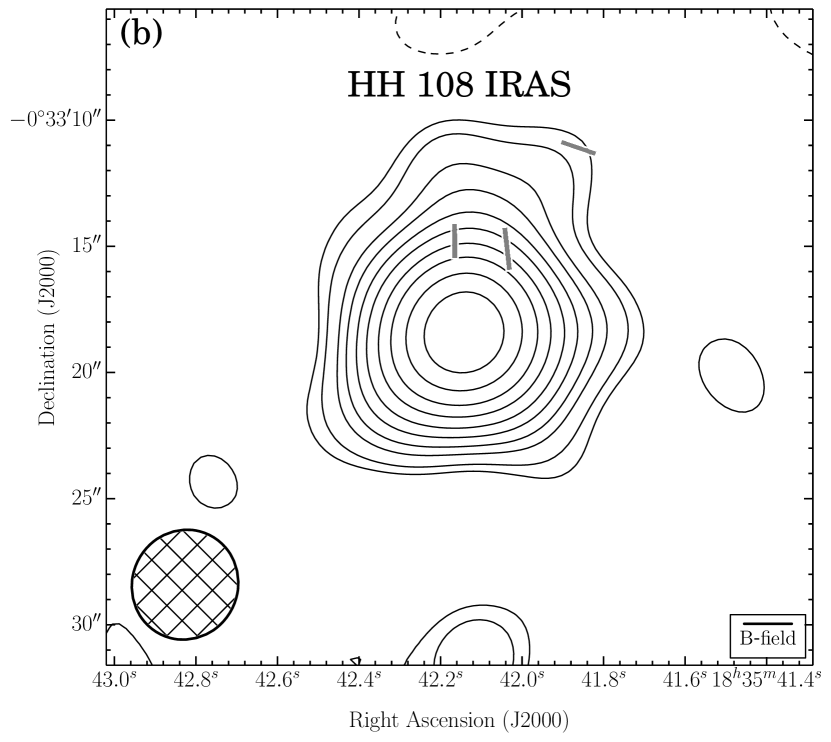
Figure 28.— HH 108 IRAS. Same as Figure 4. (a) The velocity ranges of the CO($J=2\rightarrow 1$) line wing emission are 22.3 to 13.8 km s^-1 (redshifted) and 9.6 to 2.2 km s^-1 (blueshifted). $\sigma_{\textrm{SL}}=0.86$ K km s^-1. (b) $\sigma_{I}=2.6$ mJy bm^-1. There is no (c) plot because there were no SCUBA, SHARP, or Hertz data to overlay.

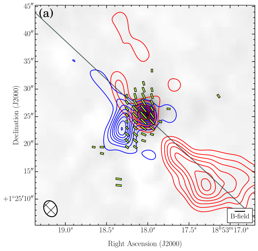
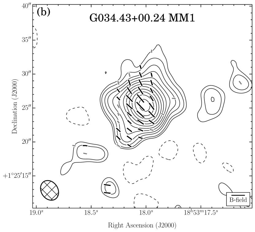
Figure 29.— G034.43+00.24 MM1. Same as Figure 4. (a) The velocity ranges of the CO($J=2\rightarrow 1$) line wing emission are 96.5 to 66.8 km s^-1 (redshifted) and 49.9 to 18.2 km s^-1 (blueshifted). $\sigma_{\textrm{SL}}=5.81$ K km s^-1. (b) $\sigma_{I}=8.8$ mJy bm^-1. There is no (c) plot because there were no SCUBA, SHARP, or Hertz data to overlay.

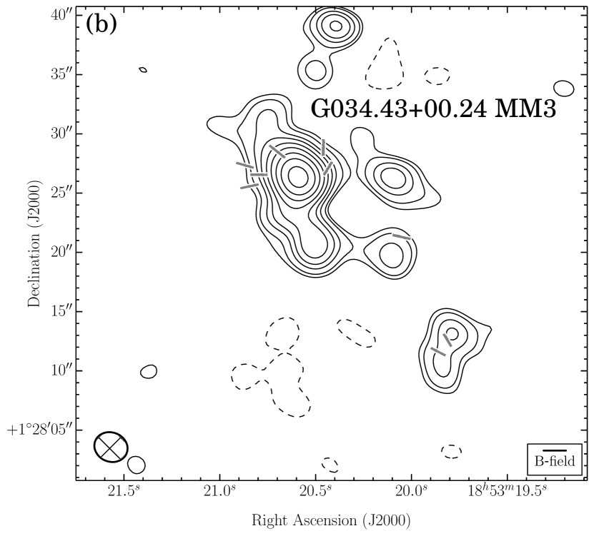
Figure 30.— G034.43+00.24 MM3. Same as above. (b) $\sigma_{I}=1.4$ mJy bm^-1. There is no (a) plot because there were no spectral-line data to plot. There is no (c) plot because there were no SCUBA, SHARP, or Hertz data to overlay.

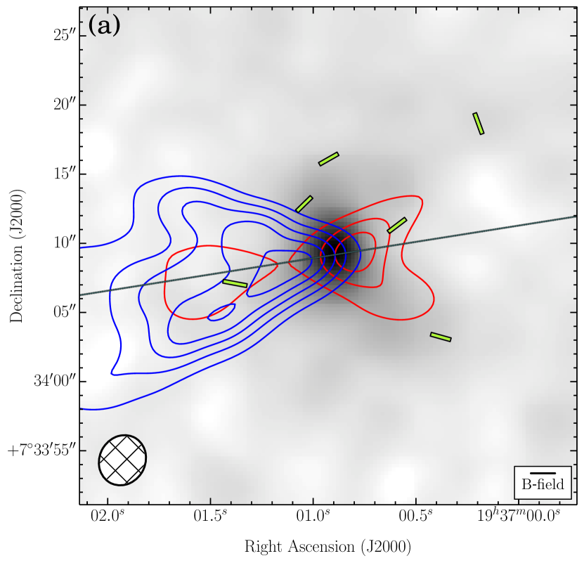
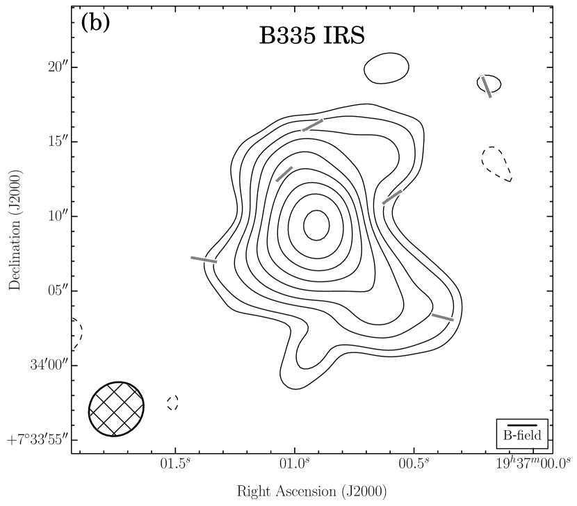
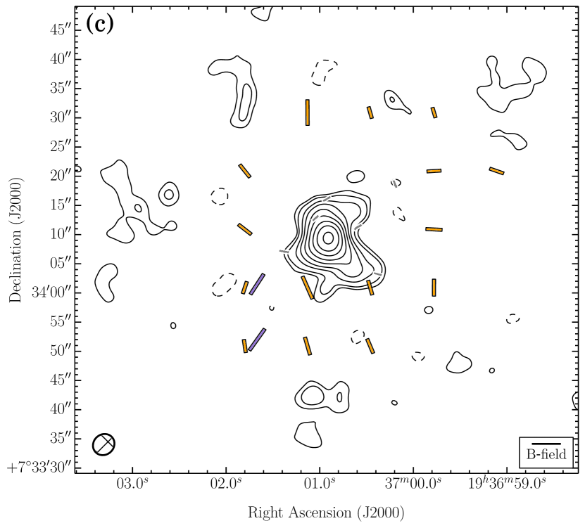
Figure 31.— B335 IRS. Same as Figure 4. (a) The velocity ranges of the CO($J=2\rightarrow 1$) line wing emission are 19.7 to 12.3 km s^-1 (redshifted) and 6.0 to –0.4 km s^-1 (blueshifted). $\sigma_{\textrm{SL}}=1.33$ K km s^-1. (b) $\sigma_{I}=1.6$ mJy bm^-1.

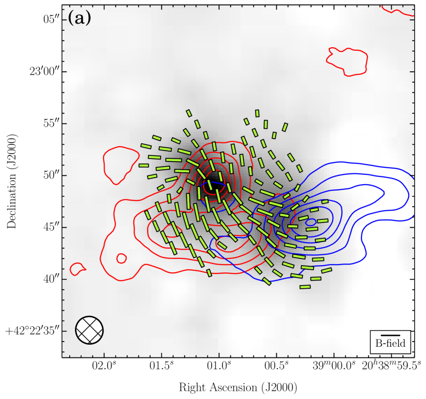
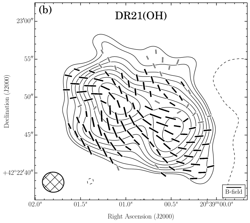
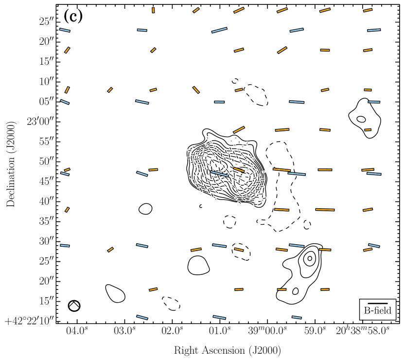
Figure 32.— DR21(OH). Same as Figure 4. (a) The velocity ranges of the CO($J=2\rightarrow 1$) line wing emission are 36.9 to 7.2 km s^-1 (redshifted) and –24.5 to –41.4 km s^-1 (blueshifted). $\sigma_{\textrm{SL}}=2.64$ K km s^-1. (b) $\sigma_{I}=8.6$ mJy bm^-1.

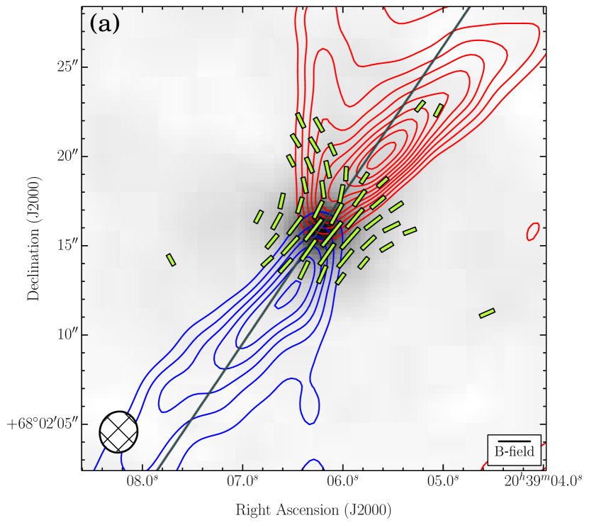
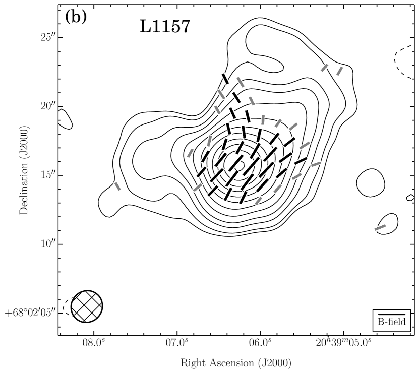
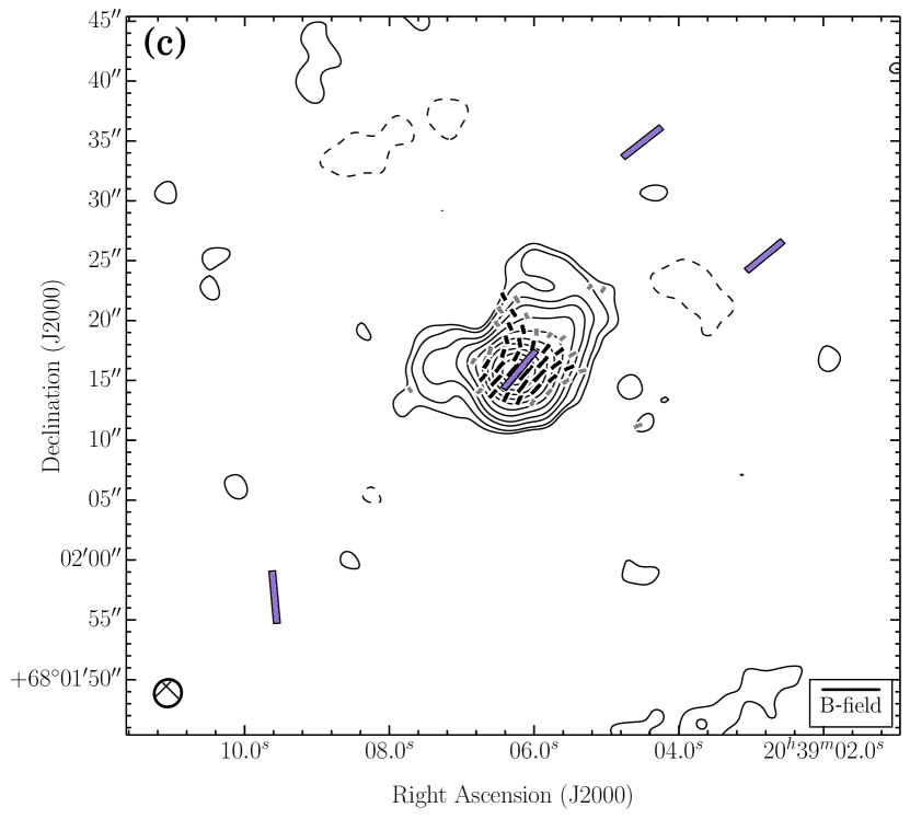
Figure 33.— L1157. Same as Figure 4. (a) The velocity ranges of the CO($J=2\rightarrow 1$) line wing emission are 14.7 to 5.2 km s^-1 (redshifted) and –2.2 to –14.9 km s^-1 (blueshifted). $\sigma_{\textrm{SL}}=2.52$ K km s^-1. (b) $\sigma_{I}=1.7$ mJy bm^-1.

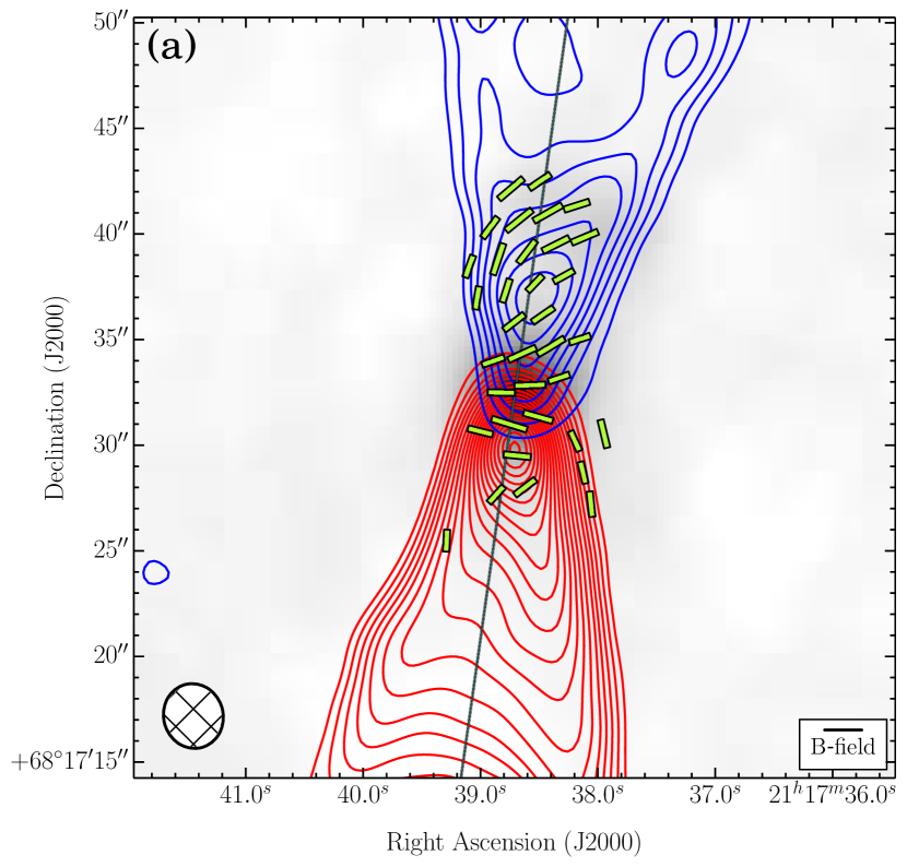
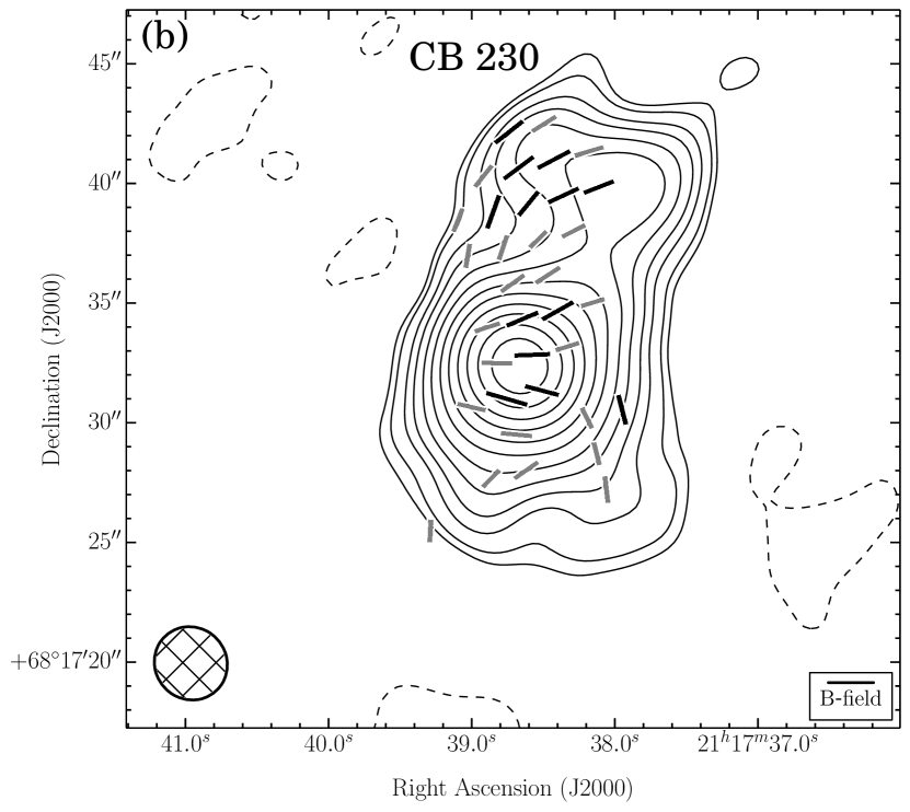
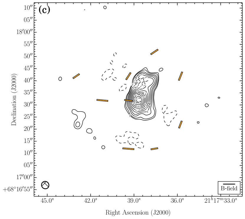
Figure 34.— CB 230. Same as Figure 4. (a) The velocity ranges of the CO($J=2\rightarrow 1$) line wing emission are 13.1 to 5.7 km s^-1 (redshifted) and –1.8 to –16.6 km s^-1 (blueshifted). $\sigma_{\textrm{SL}}=0.47$ K km s^-1. (b) $\sigma_{I}=0.7$ mJy bm^-1.

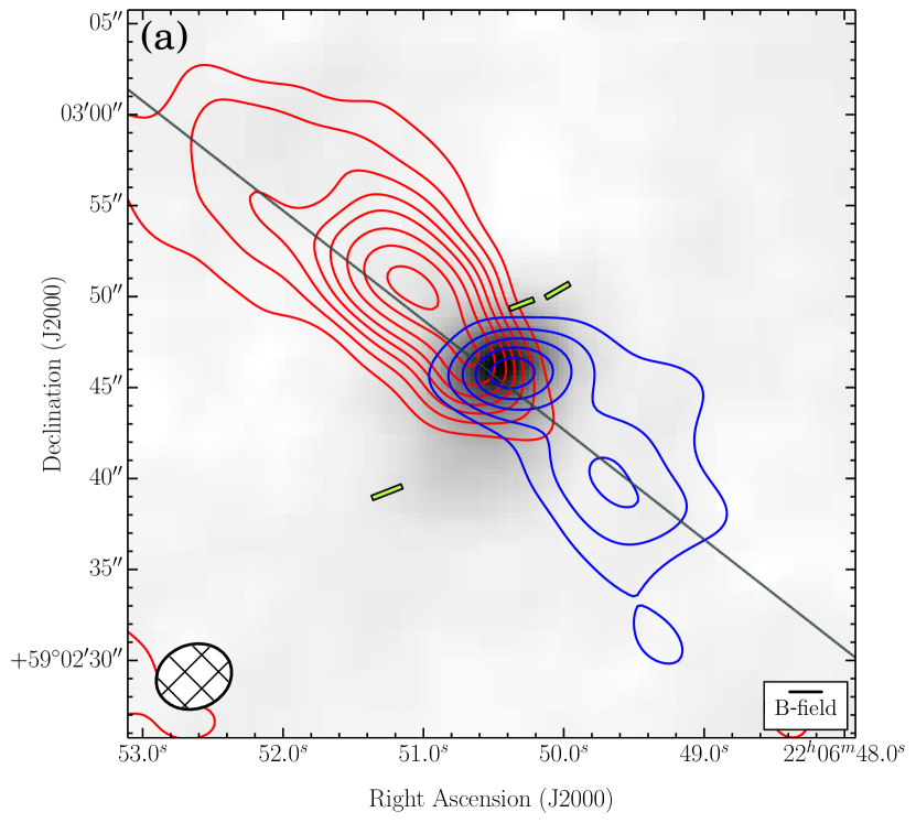
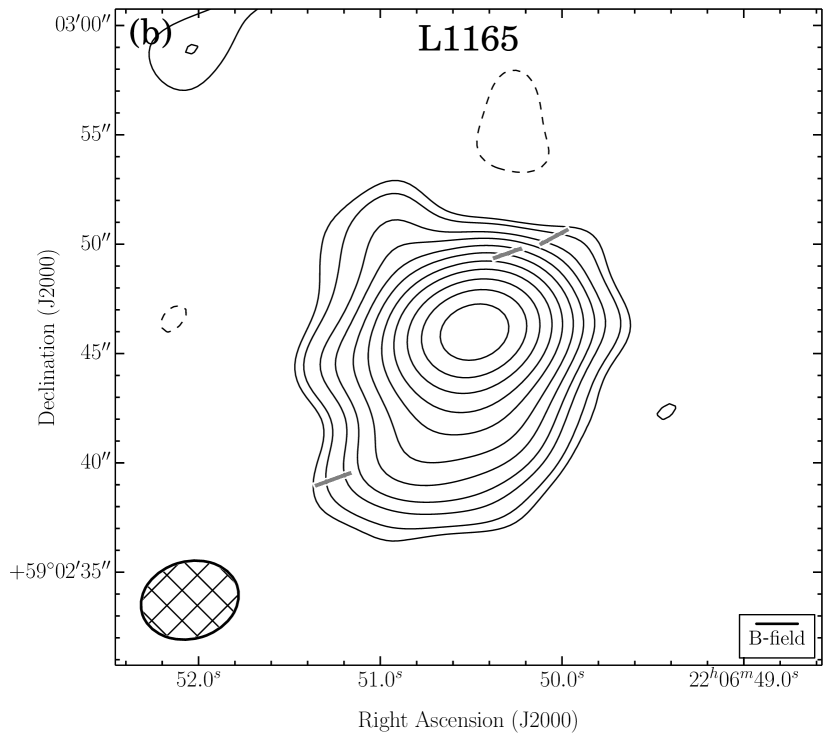
Figure 35.— L1165. Same as Figure 4. (a) The velocity ranges of the CO($J=2\rightarrow 1$) line wing emission are 4.9 to –0.4 km s^-1 (redshifted) and –2.5 to –7.8 km s^-1 (blueshifted). $\sigma_{\textrm{SL}}=0.81$ K km s^-1. (b) $\sigma_{I}=1.2$ mJy bm^-1. There is no (c) plot because there were no SCUBA, SHARP, or Hertz data to overlay.

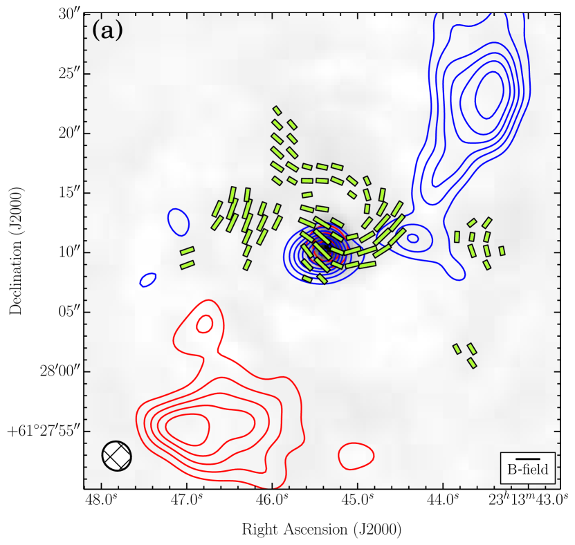
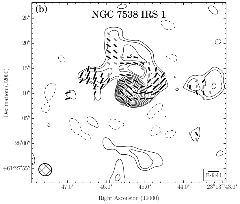
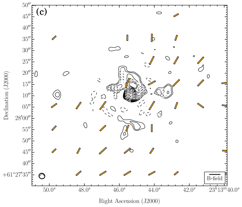
Figure 36.— NGC 7538 IRS 1. Same as Figure 4. (a) The velocity ranges of the CO($J=2\rightarrow 1$) line wing emission are –36.3 to –39.5 km s^-1 (redshifted) and –69.1 to –75.5 km s^-1 (blueshifted). $\sigma_{\textrm{SL}}=3.2$ K km s^-1. (b) $\sigma_{I}=19.3$ mJy bm^-1.

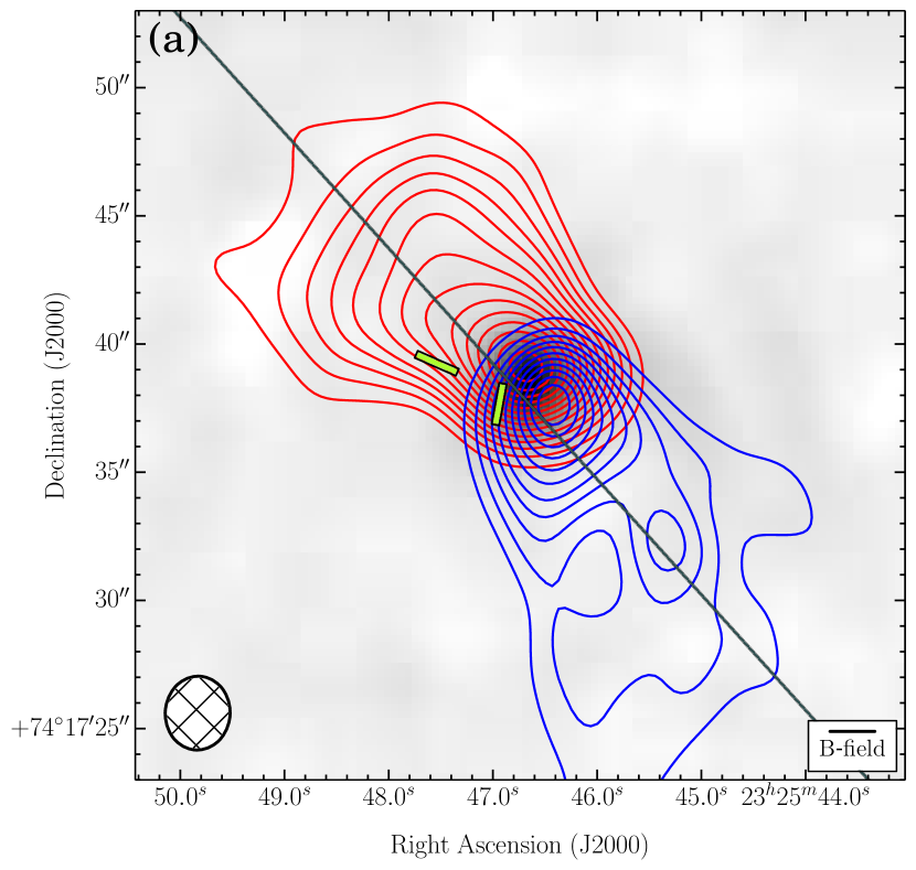
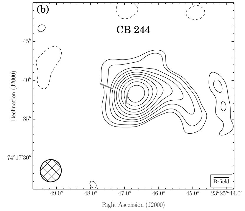
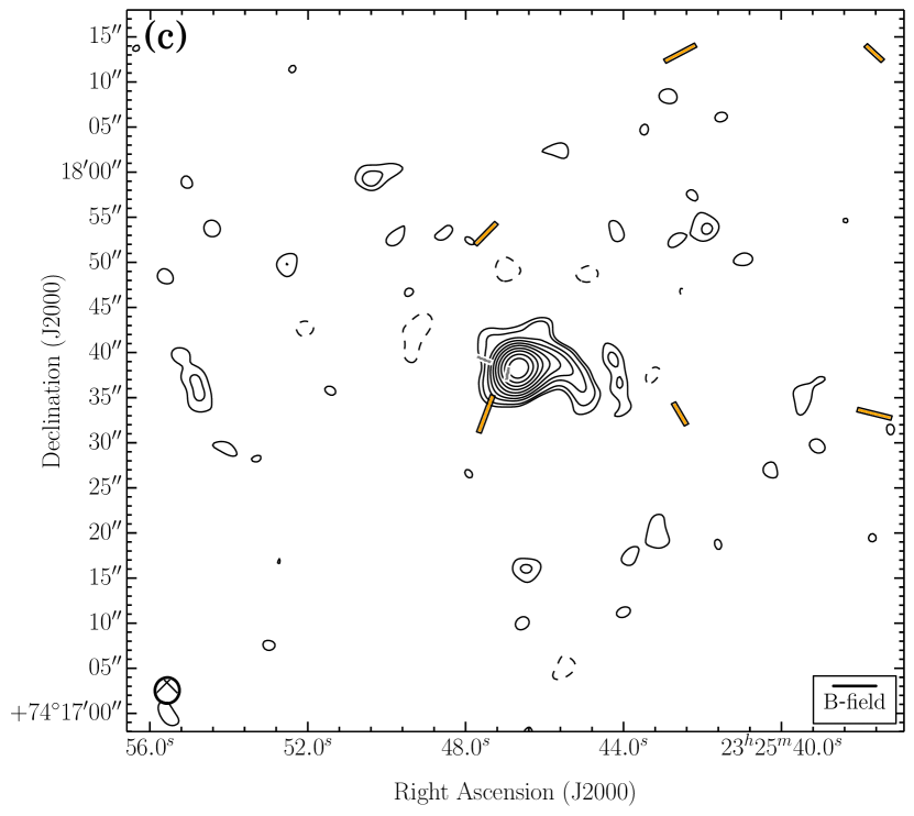
Figure 37.— CB 244. Same as Figure 4. (a) The velocity ranges of the CO($J=2\rightarrow 1$) line wing emission are 11.7 to 6.4 km s^-1 (redshifted) and 2.2 to –3.1 km s^-1 (blueshifted). $\sigma_{\textrm{SL}}=0.98$ K km s^-1. (b) $\sigma_{I}=0.6$ mJy bm^-1.

Appendix B APPENDIX B: DESCRIPTION OF SOURCES

B.1. W3 Main

The W3 molecular cloud, located at a distance of 1.95 kpc (Xu et al., 2006), is one of the massive molecular clouds in the outer galaxy, with an estimated total gas mass of 3.8$\times 10^{5}$ $\hbox{M}_{\odot}$ (Moore et al., 2007). It contains several young, massive star-forming complexes, the most active of which is W3 Main. Early thermal dust continuum observations identified three sources: W3 SMS1, SMS2, and SMS3 (Ladd et al., 1993). Our polarization observations are toward W3 SMS1 and are centered on the luminous infrared source IRS5 (2$\times 10^{5}$ $\hbox{L}_{\odot}$, Campbell et al. 1995).

Discovered by Wynn-Williams et al. (1972), IRS5 is a double infrared source (Howell et al., 1981); both sources are associated with radio continuum emission that is consistent with very young, hyper-compact H II regions (van der Tak et al., 2005). Millimeter interferometer observations have resolved the brightest dust continuum source associated with IRS5 into at least five compact cores (MM1–MM5, Rodón et al. 2008). Hubble Space Telescope observations also revealed seven near-IR sources within IRS5 (Megeath et al., 2005). Multiple outflows associated with IRS5 have also been observed in various molecular tracers (Rodón et al., 2008; Wang et al., 2012). It has been proposed that IRS5 is a Trapezium cluster in the making and thus holds valuable clues to high mass cluster formation.

Low resolution infrared and submillimeter polarization observations have revealed low polarization, with a notable decline toward IRS 5 and a spread of values away from the dust peak (Schleuning et al., 2000; Matthews et al., 2009). Water-maser polarization observations have revealed an hourglass-shaped field toward IRS5 (Imai et al., 2003).

The more extended structure to the west of IRS5 observed in our TADPOL image is the free-free emission associated with the H II region W3 B, better known for its infrared association IRS3 (Wynn-Williams et al., 1972; Megeath et al., 1996). The associated stellar source (designated as IRS3a) is consistent with a star of spectral type O6 (Megeath et al., 1996).

See Figure 4 for maps.

B.2. W3(OH)

W3(OH) is another active, high-mass star formation site in the W3 molecular cloud. H₂O maser parallax measurements place the complex at a distance of 2.04 kpc (Hachisuka et al., 2006). W3(OH) consists of two main regions: a young, limb-brightened ultra-compact (UC) H II region with several OH masers, known as W3(OH) (Dreher & Welch, 1981), and a younger, massive hot core with water masers $\sim$6 ″ east of W3(OH) known as W3(H₂O) or W3(TW) (Turner & Welch, 1984). Both of these regions are within the TADPOL field-of-view. The UC H II region is ionized by a massive O9 star, and has a total luminosity of 7.1$\times 10^{4}$ $\hbox{L}_{\odot}$ (Hirsch et al., 2012). High resolution observations have revealed dense gas in a massive protobinary system ($\sim$22 $\hbox{M}_{\odot}$) towards W3(H₂O), without any associated ionized emission from UC H II region (Wilner et al., 1999; Wyrowski et al., 1999; Chen et al., 2006). Massive, collimated outflows and jets have been detected towards the W3(H₂O) system (Reid et al., 1995; Zapata et al., 2011).

SCUBA observations show significant polarization throughout the region ($\sim$5%) with some evidence for depolarization towards the center (Matthews et al., 2009). Strong magnetic fields are also implied by single-dish CN Zeeman measurements, which find a $\sim$1.1 mG field strength towards this region (Falgarone et al., 2008).

See Figure 5 for maps.

B.3. L1448 IRS 2

L1448 IRS 2 is a Class 0 YSO (O’Linger et al., 1999) located in the Perseus molecular cloud at a distance of $\sim$ 230  pc (Hirota et al., 2011). Its well collimated bipolar outflow has been studied by CO mapping (e.g., Wolf-Chase et al., 2000), Spitzer IRAC (Tobin et al., 2007), and molecular hydrogen mapping (e.g., Eislöffel, 2000). It is also one of the objects where Kwon et al. (2009) found that dust grains have grown significantly even in the youngest protostellar stage. The surrounding flattened structure was studied by Spitzer observations (Tobin et al., 2010). Recent SHARP observations by Chapman et al. (2013) show magnetic fields that are aligned with the bipolar outflow to within $\sim$ 10$\arcdeg$.

See Figure 6 for maps.

B.4. L1448N(B)

L1448N(B) is a Class 0 YSO at the center of the L1448 IRS3 core (also called L1448N and IRAS 03225+3034) (Bachiller & Cernicharo, 1986), at a distance of $\sim$ 230 pc (Hirota et al., 2011). It was first detected at 6 cm (Anglada et al., 1989), although it is weaker at centimeter wavelengths that its companion L1448N(A), which lies $\sim$ 7$\arcsec$ to the northeast. L1448N(A) and L1448N(B) are suspected to be a gravitationally bound common-envelope binary (Kwon et al., 2006; Looney et al., 2000) with a separation of $\sim$ 2000 AU, even though they seem to be in different evolutionary stages. L1448N(B) is the stronger source at millimeter wavelengths (Terebey & Padgett, 1997; Looney et al., 2000); it appears to be younger and more embedded than its companion (O’Linger et al., 2006).

CO observations of L1448N(B) show an outflow with a position angle estimated to be 129$\arcdeg$ on large (arc-minute) scales (Wolf-Chase et al., 2000) and 105$\arcdeg$ on small scales (Kwon et al., 2006). The redshifted lobe is easy to distinguish in channel maps, but the blueshifted lobe overlaps, and may even interact with, the outflow from L1448C, $\sim$ 75$\arcsec$ to the south. High-resolution ($0.7\arcsec\times 0.5\arcsec$) maps of the 2.7 mm continuum emission from L1448N(B) show a protostellar envelope elongated in a direction nearly perpendicular ($PA\sim 56\arcdeg$) to the outflow (Looney et al., 2000). Observations of the linear polarization of 1.3 mm continuum emission made with the BIMA interferometer at $\sim 4\arcsec$ resolution (Kwon et al., 2006) imply that the magnetic field through the envelope is also approximately perpendicular to the outflow. This orientation is consistent with lower-resolution (10″) 850 $\mu$m polarization observations made with SCUPOL on the JCMT (Matthews et al., 2009).

See Figure 7 for maps.

B.5. L1448C

L1448C is the collective name for the embedded Class 0 YSOs located 75–80$\arcsec$ southeast of L1448N, at a distance of 232  pc (Hirota et al., 2011). L1448C has been the target of numerous observations in the IR continuum (e.g., Tobin et al., 2007), in the (sub)millimeter continuum (e.g., Jørgensen et al., 2007), in CO line emission (e.g., Nisini et al., 2000), and in SiO line emission (e.g., Nisini et al., 2007) because it is the point of origin of symmetrical, well collimated, high-velocity, and rapidly evolving (Hirano et al., 2010) outflows. The blueshifted outflow lobe extends to the north; the westward bend in the outflow at the point where it overlaps L1448N is strong evidence that the L1448C and L1448N outflows interact (Bachiller et al., 1995).

The multiplicity of YSOs in L1448C was revealed by observations of millimeter continuum emission (Volgenau, 2004). The strongest millimeter source, called L1448C(N) (Jørgensen et al., 2006) or L1448mm A (Tobin et al., 2007), is the likely source of the outflows. A second source, $\sim$ 8$\arcsec$ south of L1448mm A, is weaker in millimeter emission but prominent in maps of near- and mid-infrared emission made with IRAC and MIPS, respectively, on Spitzer. This source is called L1448C(S) (Jørgensen et al., 2006) or L1448mm B (Tobin et al., 2007).

SCUBA maps of linearly polarized 850 $\mu$m emission from the L1448 cloud only show significant polarization along the perimeter of the clump of 850 $\mu$m continuum emission coincident with L1448C. There is no obvious trend in the orientation of the magnetic field lines.

See Figure 8 for maps.

B.6. L1455 IRS 1

The dark cloud L1455 is located $\sim$1$\degree$ south of the active star formation region NGC 1333 at a distance of 320 pc (de Zeeuw et al., 1999). L1455 IRS 1 (also known as L1455 FIR and IRAS 03245+3002) is the brightest far infrared source in the cloud. It is a low mass, Class I protostar, which was first detected in the far infrared with the Kuiper Airborne Observatory (Davidson & Jaffe, 1984). High velocity CO emission was first detected by Frerking & Langer (1982) and was first mapped in CO($J=1\rightarrow 0$) by Goldsmith et al. (1984), who found extended blue- and redshifted emission over an area of more than 10$\arcmin$, indicating the presence of more than one outflow, which they thought might be powered by RNO 15 and/or L1455 IRS 1. More recent studies (Hatchell et al., 2007; Curtis et al., 2010) have identified 4 outflows in L1455, each associated with a submillimeter core.

L1455 IRS 1 was first imaged in narrowband H₂S(1) emission by Davis et al. (1997), who found three compact H₂ knots on the symmetry axis of IRS 1, outlining a highly collimated outflow at a position angle of 32$\degree$, while Curtis et al. (2010) determined a position angle of 42$\degree$ from their CO($J=3\rightarrow 2$) imaging. This agrees well with the TADPOL CO($J=2\rightarrow 1$) imaging, which shows a well-defined bipolar molecular outflow. Although the dust polarization is not very strong, it is still a case where the B-field appears to be perpendicular to the outflow.

See Figure 9 for maps.

B.7. NGC 1333-IRAS 2A

The IRAS 2 (IRAS 03258+3104) core lies approximately 11$\arcmin$ south-southwest of the center of the NGC 1333 reflection nebula, at a distance of 320 pc (de Zeeuw et al., 1999). IRAS 2 hosts at least three deeply embedded YSOs (Sandell & Knee, 2001). IRAS 2A, the strongest emitter at (sub)millimeter wavelengths, is a Class 0 object near the center of the core (Lefloch et al., 1998), at the intersection of nearly perpendicular CO outflows (Sandell et al., 1994; Engargiola & Plambeck, 1999). One outflow (position angle $\sim$ 104$\degree$), with a blueshifted lobe that extends $\sim$ 100$\arcsec$ to the west and a redshifted lobe that extends $\sim$ 85$\arcsec$ to the east, is highly collimated and presumably young. The other outflow (position angle $\sim$ 25$\degree$), with blueshifted (south) and redshifted (north) lobes that extend at least 70$\arcsec$ in either direction, is poorly-collimated and older. The coincidence of IRAS 2A with the point of origin of the outflows suggests that IRAS 2A is an unresolved ($<65$ AU) binary system (e.g., Jørgensen et al., 2004).

The magnetic field across the IRAS 2 core, as mapped with the SCUPOL on the JCMT (14$\arcsec$ resolution), was described as weak with a “random field pattern” (Curran et al., 2007). However, higher resolution (3$\arcsec$) data obtained by Curran et al. with the BIMA (Berkeley Illinois Maryland Array) interferometer shows magnetic field line with a roughly east-west orientation across most of the emitting region, which is consistent with the TADPOL observations.

See Figure 10 for maps.

B.8. SVS 13

SVS 13 was discovered as a near-infrared source by Strom et al. (1976) in the NGC 1333 star forming region. Using VLBI observations of 22 GHz H₂O masers, Hirota et al. (2008) found a distance of 235 pc. Observations at millimeter wavelengths reveal at least three continuum sources within SVS 13. These sources, which form a straight line in the plane of the sky from northeast to southwest, have been named as A, B, and C, respectively (Looney et al., 2000, and references therein). Source A is a Class 0/I source coincident with the infrared/optical counterparts of SVS 13; sources B and C are Class 0 sources. High resolution BIMA observations revealed a weak component of source A that is located 6″ to the southwest of the source and is coincident with centimeter continuum source VLA3 (Rodriguez et al., 1997; Rodríguez et al., 1999). TADPOL observations focus on sources A and B.

Observational evidence suggests that SVS 13 is powering the well studied chain of Herbig-Haro (HH) objects HH 7–11 (Bachiller et al., 2000; Looney et al., 2000). However, there is some debate as to the main exciting source of the outflow, which could be either VLA3 or SVS 13 (Rodriguez et al., 1997). This object is known to be one of the brightest H₂O maser sources among the known low-mass YSOs (Haschick et al., 1980; Claussen et al., 1996; Furuya et al., 2003).

See Figure 11 for maps.

B.9. NGC 1333-IRAS 4A

NGC 1333-IRAS 4A comprises two deeply embedded Class 0 YSOs at the south end of the NGC 1333 reflection nebula, located at a distance of 320 pc (de Zeeuw et al., 1999). The binarity of IRAS 4A, first detected in 0.84 mm CSO-JCMT baseline data (Lay et al., 1995), has been resolved interferometrically at millimeter (Looney et al., 2000), submillimeter (Jørgensen et al., 2007), and centimeter (Reipurth et al., 2002) wavelengths. The two components are 1.8$\arcsec$ apart (580 AU at 320 pc) and share a common envelope with an estimated mass of 2.9 $M_{\sun}$ (Looney et al., 2003). High-resolution observations of molecular line emission from IRAS 4A have revealed both low-density (Jørgensen et al., 2007) and high-density (Di Francesco et al., 2001) tracers with inverse P-Cygni profiles, which have been interpreted as evidence that envelope material is falling onto the central protostars.

The outflows emanating from IRAS 4A have been mapped in several CO transitions (e.g., Blake et al., 1995; Knee & Sandell, 2000; Jørgensen et al., 2007; Yıldız et al., 2012). The outflows are well collimated but are “bent” in the sky plane. Close ($<0.5\arcmin$) to IRAS 4A, the outflows are oriented north-south; further from the protostars, the outflows have a position angle or $\sim 45\arcdeg$. The redshifted lobe extends northward, and the blueshifted lobe extends southward. The extent of the outflows on the sky ($4\arcmin$) and the large range of line-of-sight velocities suggests that the outflow axis has an inclination $<45\arcdeg$.

Maps of linearly polarized dust emission from IRAS 4A have been made at 850 $\mu$m with the SCUBA polarimeter on the JCMT (Matthews et al., 2009). These maps imply a large-scale magnetic field that is fairly uniform in the northeast-southwest direction across the IRAS 4 core. Girart et al. (2006) also mapped IRAS 4A at high resolution with the Submillimeter Array (SMA), revealing one of the first “hourglass” B-field morphologies ever seen in a low-mass protostar.

See Figure 12 for maps.

B.10. NGC 1333-IRAS 4B and 4B2

NGC 1333-IRAS 4B and 4B2 are Class 0 sources in Perseus at a distance of 320 pc (de Zeeuw et al., 1999), and about 30″ to the southeast of the well known Class 0 source NGC 1333-IRAS 4A. IRAS 4B hosts a slow ($\sim$10 km s^-1) bipolar molecular outflow oriented north-south. Single-dish maps from the SCUBA (Matthews et al., 2009) and Hertz (Dotson et al., 2010) polarimeters show polarization consistent with the prominent polarization detected by CARMA on the western edge of the core.

Strong water lines were detected toward IRAS 4B by the Spitzer infrared spectrograph (Watson et al., 2007) and Herschel HIFI (Herczeg et al., 2012). Watson et al. (2007) attributed the emission to shocked material falling from the protostellar envelope onto the dense surface of the circumstellar disk, which requires that the disk of IRAS 4B be oriented roughly face-on, thus allowing emission to escape from the cavity evacuated by the bipolar outflow. That assumption was called into question after VLBI measurements of the proper motions of water masers in the outflow of IRAS 4B that suggest that the object is in fact viewed edge-on (Marvel et al., 2008). The claim by Watson et al. (2007) that the water emission originates in the disk has been challenged by Herczeg et al. (2012), who argue that the emission originates in shocks within the bipolar outflow cavity.

IRAS 4B2 (also called IRAS 4BE, IRAS 4B^′, and IRAS 4BII) is the weaker binary companion 10$\arcsec$ to the east of IRAS 4B. The source has been called IRAS 4C as well (e.g., Choi et al., 1999; Looney et al., 2000), but 4C is generally used as the name of a source $\sim$40″ east-northeast of IRAS 4A (e.g., Rodríguez et al., 1999; Smith et al., 2000; Sandell & Knee, 2001). In their BIMA observations, Choi et al. (1999) saw IRAS 4B2 as an unresolved extension of continuum emission to the east of IRAS 4B. Sandell & Knee (2001) and Di Francesco et al. (2001) later resolved the 10$\arcsec$ IRAS 4B/IRAS 4B2 binary using the JCMT and the PdBI, respectively.

While prior to the TADPOL survey no spectral line emission had been detected toward IRAS 4B2, we see a small, faint E–W outflow in CO($J=2\rightarrow 1$).

See Figure 13 for maps.

B.11. HH 211 mm

HH 211 mm is the Class 0 YSO (Froebrich, 2005) launching the well-known bipolar outflow HH 211. It is located in the IC 348 cluster at the eastern part of the Perseus molecular cloud, at a distance of 320 pc (de Zeeuw et al., 1999). The jet HH 211 was relatively recently detected by near-IR H₂ observations (McCaughrean et al., 1994). Gueth & Guilloteau (1999) showed that the driving object is HH 211 mm, and they distinguished between the collimated jet and the slow extended outflow components using interferometric millimeter-continuum and CO observations. The bipolar outflow has been studied extensively in various molecular line transitions (e.g., SiO($J=1\rightarrow 0$); Chandler & Richer, 2001), and recently Spitzer IRS observations showed that the bipolar outflow material is mostly molecular (Dionatos et al., 2010). Based on the bipolar outflow velocity and extension, the kinematic age is estimated to be only $\sim$ 1000 yr. (e.g, Gueth & Guilloteau, 1999). Recent submillimeter interferometric observations have revealed that the object is a protobinary system separated by about $0.3\arcsec$ (Lee et al., 2009), and the kinematic structure of the envelope has been studied by CARMA N₂H⁺ observations (Tobin et al., 2011). The SCUPOL map toward the HH 211 and IC 348 region showed polarization that is neither aligned with nor perpendicular to the the bipolar outflow (Matthews et al., 2009).

See Figure 14 for maps.

B.12. DG Tau

DG Tau is a Class II, 0.67 M_☉ K5-M0 T Tauri star (Güdel et al., 2007, and references therein) located at a distance of roughly 140 pc in the Taurus-Auriga star-forming association (Kenyon et al., 1994; Torres et al., 2009). It is remarkable primarily for its well collimated jet, HH 158, and was among the first T Tauri stars known to exhibit such strong and clear accretion and outflow activity (Mundt & Fried, 1983). The literature on its jet is correspondingly vast, as it has been studied extensively across the electromagnetic spectrum (see, e.g., Schneider et al., 2013; Rodríguez et al., 2012b; Lynch et al., 2013, and references therein). DG Tau is properly known as DG Tau A, since it has a common proper motion companion DG Tau B, a Class I source that launches the HH 159 jet (e.g., Rodríguez et al., 2012a).

The dust disk around DG Tau has the dubious distinction of being the most frequently observed by (sub)millimeter polarimeters. It was one of the first two T Tauri disks that seemed to exhibit a tentative (3 $\sigma$) detection of unresolved 850 $\mu$m polarization using the single-dish JCMT (Tamura et al., 1999), apparently indicating a large-scale toroidal magnetic field threading the disk. Follow-up observations at 350 $\mu$m with the CSO did not confirm the 3% polarization fraction, but the wavelengths were too widely separated to rule out a spectral dependence of the polarization fraction (Krejny et al., 2009). As part of the TADPOL survey the JCMT detection was followed up at 1.3 mm using the CARMA polarimeter, which again resulted in a sensitive non-detection (Hughes et al., 2013). The CARMA results indicate that either the JCMT detection was spurious or the polarization originates from large spatial scales that are filtered out by the interferometer—an envelope, perhaps—rather than from the circumstellar disk itself.

See Figure 15 for maps.

B.13. L1551 NE

L1551 NE is a low-mass Class I protostar first discovered with IRAS (Emerson et al., 1984) and located a few arcminutes from L1551 IRS5 and at a distance of 140 pc (Kenyon et al., 1994). L1551 NE is a binary system with a bipolar molecular outflow and a Keplerian circumbinary disk (Moriarty-Schieven et al., 1995; Rodriguez et al., 1995; Reipurth et al., 2002; Takakuwa et al., 2012). SCUBA 850 $\micron$ measurements show polarization orientations in the extended dust envelope that are mostly perpendicular to the outflow direction, with no polarization detected at the continuum peak (Matthews et al., 2009). Our TADPOL observations show a clear pattern of polarization across the continuum peak, with B-field orientations perpendicular to the outflow direction.

See Figure 16 for maps.

B.14. L1527

L1527 is a Class 0/I YSO located in the Taurus molecular cloud at a distance of about 140 pc (e.g., Andre et al., 2000). Its bipolar outflow is oriented in the east-west direction and is nearly in the plane of the sky, which makes the object an ideal target for studying the disk and outflow structure at the earliest stage of low mass star formation (e.g., Jørgensen et al., 2007). Recently the disk was revealed to have Keplerian motion, and the protostellar mass was estimated to be $\sim$ 0.2 M_☉ using CARMA ¹³CO observations (Tobin et al., 2012). In addition, detailed modeling of SMA and CARMA continuum observations found that the disk is large (about 125 AU in radius) and is thicker than the hydrostatic equilibrium case (Tobin et al., 2013a).

The source’s orientation is also beneficial for magnetic field studies. SCUPOL detected quite irregular polarization at 850 $\mu$m, but at the center the B-field orientation is perpendicular to the bipolar outflow (Matthews et al., 2009), consistent with the TADPOL observations. In contrast, SHARP detected polarization in the outer regions at 350 $\mu$m that was consistent with B-fields that are aligned with the bipolar outflow (Davidson et al., 2011).

See Figure 17 for maps.

B.15. CB 26

CB 26 (Clemens & Barvainis, 1988) is a Bok globule generally accepted to be associated with the Taurus-Auriga complex a distance of 140 pc (Launhardt & Sargent, 2001; Henning et al., 2001). The embedded YSO located near the edge of the globule is a Class I source with a luminosity of 0.5 $L_{\sun}$ (Stecklum et al., 2004). Millimeter interferometric observations of dust continuum and molecular spectral line emission (Launhardt & Sargent, 2001) show both an edge-on disk that sits at the center of a near-infrared bipolar reflection nebula (Stecklum et al., 2004), as well as a bipolar outflow (Launhardt et al., 2009) perpendicular to the disk.

SCUBA 850 $\micron$ measurements show polarization orientations both predominantly parallel to the disk (Henning et al., 2001) and predominantly perpendicular to the disk (Matthews et al., 2009). Our TADPOL observations detect polarization near the dust peak that is consistent with the latter SCUBA results.

See Figure 18 for maps.

B.16. Orion-KL

Orion-KL, the Kleinmann-Low Nebula in Orion, is the nearest region of high mass star formation, 415 pc away (Menten et al., 2007). It lies inside Orion Molecular Cloud 1 (OMC1), which in turn forms part of an integral shaped filamentary cloud that is more than 7 pc long (Johnstone & Bally, 1999). Our map, a mosaic of 7 pointings, covers Orion-KL and its associated hot core, and a piece of the more quiescent “northern ridge” about $25\arcsec$ to the NE.

At least two massive stars, Source I (SrcI) and the Becklin-Neugebauer Object (BN) are associated with Orion-KL. Proper motion measurements show that these two stars are recoiling from one another at 35–40 km s^-1; they appear to have been ejected from a multiple system just 500 years ago (Gómez et al., 2008; Goddi et al., 2011). This explosive event also is thought to have created a set of bow shocks and fingers that form a poorly collimated, NW-SE high velocity outflow; a separate, lower velocity outflow emerges from SrcI in the perpendicular direction (Plambeck et al., 2009).

Extensive polarization maps from SCUBA, Hertz, and Stokes (Dotson et al., 2000) show that the large-scale magnetic field in OMC1 is perpendicular to the long axis of the molecular cloud, with evidence for an hourglass-shaped pinch centered on KL (Schleuning, 1998). Higher resolution 345 GHz SMA observations show a remarkable circularly symmetric polarization pattern centered between SrcI and BN, near the site of the putative explosive event; a possible interpretation is that the explosion dragged the magnetic field outward into a radial pattern (Tang et al., 2010). However, within 500 AU of SrcI the magnetic field deduced from SiO v=0 maser polarization observations is relatively straight. (Plambeck et al., 2003). The B-field orientation is highly uncertain because maser polarization may be either parallel or perpendicular to the field, and because of possible Faraday rotation by foreground plasma; Plambeck et al. argued that it is at PA 145^∘, roughly perpendicular to the low velocity outflow from SrcI.

The TADPOL map shows the radial magnetic field pattern previously detected with the SMA. Our map extends further north, and shows that the magnetic field orientation in the northern ridge cloud is consistent with the large scale field, except near the SW tip where it forms part of the radial pattern.

See Figure 19 for maps.

B.17. OMC3 MMS5 and MMS6

MMS5 and MMS6 are condensations in Orion Molecular Cloud 3 (OMC3)—a narrow ridge or filament about 1 pc long and at a distance of 415 pc (Menten et al., 2007). MMS6 is the brightest millimeter continuum source in OMC3, with an estimated mass of 36 M_☉ (Chini et al., 1997b). It contains a compact core, MMS6-main, that probably is heated by an extremely young intermediate mass Class 0 protostar (Takahashi et al., 2012). A bipolar outflow, with a total length of only $4^{\prime\prime}$ (2000 AU), emerges along a N-S axis from MM6-main; the dynamical age of the outflow is less than 100 years (Takahashi & Ho, 2012). A more extended outflow emerges along an E-W axis from MMS5.

The large scale magnetic field orientation in OMC3 inferred from SCUBA data is perpendicular to the long axis of the cloud. Matthews et al. (2001) argue that the pattern of depolarization along the central axis is best explained by a field toroidally wrapped around a filament, rather than by a straight field perpendicular to a sheet. The field orientations that we measure for both the MMS5 and MMS6 cores are closely aligned with the large-scale field. Our results for MMS6 agree well with previous $3.6^{\prime\prime}$ resolution observations of this source made with BIMA (Matthews et al., 2005).

See Figure 20 for maps.

B.18. OMC2-FIR3 and 4

OMC2 is an intermediate mass star-forming region located north of the massive OMC1 complex in the so-called integral-shaped filament of Orion A. Located at a distance of 415 pc (Menten et al., 2007), it is one of the brightest regions in the Orion Nebula and is know to harbor several protostellar objects and pre-main-sequence stars. Earlier continuum studies at (sub)millimeter wavelengths have established it to be in a later evolutionary stage of star formation than the OMC3 region neighboring it to the north (Chini et al., 1997b; Lis et al., 1998). More recent studies have modeled several of its embedded sources as infalling protostars, young stars with disks, and binaries comprising both types of objects (Adams et al., 2012). More specifically, although OMC2-FIR4 is well modeled as a Class 0 protostar of approximately $50\,L_{\sun}$ and $10^{-4}M_{\sun}\,\mathrm{yr}^{-1}$ mass infall rate (Adams et al., 2012), recent high resolution measurements have resolved three spatially distinct sources in its core (López-Sepulcre et al., 2013).

The polarization of the OMC2 region and the FIR3 and 4 sources was first investigated at 350 $\mu$m by Houde et al. (2004) with Hertz at the CSO (see also Dotson et al. 2010). This region is characterized by extremely low polarization levels as well as a strong depolarization with increasing total intensity. For example, OMC2-FIR4 was found to have a mean polarization of $0.35\%\pm\,0.08\%$ within region of approximately $\pm$ 0.3$\arcmin$ from its peak (200 Jy within a beam of $20\arcsec$ FWHM at 350 $\micron$), making it one of the most weakly polarized molecular cloud complexes ever observed at that wavelength. Although higher polarization was measured at 850 $\micron$, the relatively low polarization as compared with other sources within the integral-shaped filament was confirmed by Matthews et al. (2009) and Poidevin et al. (2010). OMC2-FIR4 was also observed to be a region of transition in the orientation of the polarization. The mean polarization angle goes from $\sim$ 115^∘ south of it to $\sim$ 175^∘ to the north at OMC2-FIR3, where the polarization angle is relatively well aligned with the filament. This transition region is almost coincident with a location of intense outflow activity reported by Williams et al. (2003).

The aforementioned low levels of polarization obtained with single-dish measurements are in contrast with the results shown in Table IV and Figure 21, where mean polarization fractions of $\sim$ 6–8% are detected with CARMA, making FIR 3 and 4 two of the most polarized sources in our sample. This may be reconciled by the fact that the magnetic field, as measured at small scales with CARMA, significantly changes its orientation within just a few arcseconds towards the center of the map (i.e., at OMC2-FIR4). The change of nearly $90^{\circ}$ observed could account for the exceedingly low polarization observed with Hertz, if the data were combined within a single Hertz beam.

See Figure 21 for maps.

B.19. CB 54

CB 54 (LBN1042; Lynds 1965; Clemens & Barvainis 1988) is a Bok globule at a distance of 1.1 kpc (Henning et al., 2001, and references therein). (Sub)millimeter and mid-infrared observations reveal two Class I YSOs coincident with source IRAS 07020-1618, with strong dust continuum emission and one or two bipolar outflows (Yun & Clemens, 1994; Zhou et al., 1996; Ciardi & Gómez Martín, 2007; de Gregorio-Monsalvo et al., 2009; Launhardt et al., 2010). SCUBA 850 $\micron$ measurements show weak polarization across the continuum source, with changing orientation and increased strength in the envelope (Henning et al., 2001; Matthews et al., 2009).

See Figure 22 for maps.

B.20. VLA 1623

VLA 1623 is the prototypical Class 0 source, discovered by Andre et al. (1993). It is located in the southern edge of the Ophiuchus A cloud at a distance of 125 pc (Loinard et al., 2008). It has a highly collimated outflow, as is typical of Class 0 sources, and this outflow extends over a large distance at a common position angle (Andre et al., 1990). The polarization toward VLA 1623 was measured by Holland et al. (1996) using the single bolometer UKT14, and the B-field was found to be perpendicular to the CO outflow. Holland et al. (1996) note that this alignment of the field implies that the large-scale field in the cloud cannot therefore collimate the outflow. The single dish polarization data from SCUBA (Matthews et al., 2009) and Hertz (Dotson et al., 2010) are consistent with this early picture, as are the CARMA data, which show that the central region has a preferred B-field orientation orthogonal to the outflow. This central region may be a flattened pseudo-disk, as discussed for other Class 0 sources by Davidson et al. (2011). The orientation of the field is aligned along the major axis of this pseudo-disk and orthogonal to the outflow, and even follows the emission extension to the north east. While the field orientation on small scales might alone suggest a toroidal field component, we note that in fact the CARMA field orientations are consistent with those of the large-scale emission.

See Figure 23 for maps.

B.21. Ser-emb 1, 6, 8, 8(N), and 17

Ser-emb 1, 6, 8, 8(N), and 17 are low-mass, Class 0 (Ser-emb 6, 8, 8(N), 17) and Class I (Ser-emb 1) protostars in the Serpens Main cluster, located at a distance of 415 pc (Dzib et al., 2010). All sources are discussed in Enoch et al. (2011), who made high-resolution 1.3 mm maps of nine low-mass cores in Serpens using CARMA. The results in Enoch et al. (2011) follow up on a large 1.1 mm survey of protostars using Bolocam on the CSO (Enoch et al., 2007).

Ser-emb 6 (also called Serp-FIR1 and Serp-SMM1) is the brightest (sub)millimeter source in the Serpens Main cluster. It harbors a Class 0 protostar at its center. Continuum observations at 6 cm using the Karl G. Jansky Very Large Array (VLA) resolved the continuum peak into three collinear sources, where the NW and SE components appear to be moving away from the central source (Rodriguez et al., 1989). While the three sources are not obviously present in the 1.3 mm maps from Enoch et al. (2011), it is possible that the outer two are associated with the lobes of the complicated bipolar outflow, which may be causing the disturbed B-field morphology on the E and W edges of the TADPOL map. The large-scale polarization properties of Ser-emb 6 are discussed at length in Chapman et al. (2013), who note that the polarization they measure with SHARP is not consistent with the small-scale morphology measured by CARMA. This could be because of projection effects, as the source and its complicated bipolar outflow are thought to be viewed at a high inclination angle with respect to the sky (Enoch et al., 2009).

Ser-emb 8 is also called S68N by McMullin et al. (1994), who examined the chemistry in the Serpens Main region. The two sources are notable for having the most distinct, well collimated SiO($J=5\rightarrow 4$) bipolar outflows in the entire TADPOL sample. It is also interesting to note that despite lying only $\sim$ 10$\arcsec$ apart from one another, the pair of cores exhibit B-fields and outflows that are both parallel (Ser-emb 8) and perpendicular (Ser-emb 8(N)).

See Figures 24, 25, 26, and 27 for maps.

B.22. HH 108 IRAS

HH 108 IRAS (also known as IRAS 18331-0035) is a Class 0/I YSO (Froebrich, 2005) in the Serpens molecular cloud, at a distance of about 310 pc (de Lara et al., 1991). The object was identified by 1.3 mm observations (Chini et al., 1997a) following the detection of the Herbig-Haro object HH 108 (Reipurth & Eiroa, 1992). A colder millimeter object was discovered $70\arcsec$ northeast of HH 108 IRAS, and was named HH 108 MMS (Chini et al., 1997a). An elongated structure enclosing these two objects was also detected in submillimeter observations (Chini et al., 2001). Recently, Tobin et al. (2011) reported IRAM 30 m and CARMA data of N₂H⁺ showing a velocity gradient perpendicular to the bipolar outflow. Siebenmorgen & Krügel (2000) have detected polarization of scattered light toward HH 108 IRAS and HH 108 MMS at 14 $\mu$m, which shows magnetic fields aligned with the elongated structure enclosing the two objects. However, no previous polarimetric observations of thermal dust emission have been reported toward this region.

See Figure 28 for maps.

B.23. G034.43+00.24 MM1 and MM3

G034.43+00.24 is a massive star-forming region associated with the IRAS source IRAS 18507$+$0121, located at a distance of 1.56 kpc (Kurayama et al., 2011). The most prominent source in the complex is the UC H II region G34.4$+$0.23, which is embedded in a massive (1000 $\hbox{M}_{\odot}$) dense core (Miralles et al., 1994; Molinari et al., 1996; Bronfman et al., 1996). At $\sim$ 5 $\arcsec$ resolution, 3 mm spectral line and continuum observations revealed another massive ($\sim$240 $\hbox{M}_{\odot}$) dense core north of the UC H II region known as G34.4MM. Near-infrared non-detection and the lack of a significant radio counterpart suggested a deeply embedded, high-mass protostar (Shepherd et al., 2004). Further millimeter continuum and Spitzer mid-IR observations revealed that the region is located in an $\sim$8 $\arcmin$ long infrared dark cloud known as MSXDC G034.43+00.24 (Rathborne et al., 2005). Rathborne et al. identified four compact millimeter clumps labeled MM1–MM4, with MM1 corresponding to the millimeter core G34.4MM mentioned above. TADPOL observations focused on the cores MM1 and MM3.

The estimated masses and luminosities are 800 $\hbox{M}_{\odot}$ and 32000 $\hbox{L}_{\odot}$ for MM1, and 170 $\hbox{M}_{\odot}$ and 12000 $\hbox{L}_{\odot}$  for MM3 (Rathborne et al., 2005). SMA continuum observations at much higher resolution show that MM1 is a 29 $\hbox{M}_{\odot}$ unresolved core with hot-core-like line emission (Rathborne et al., 2008). Recent ALMA observations by Sakai et al. (2013) show that MM3 is a hot core with a mass of $\lesssim 1.1$ $\hbox{M}_{\odot}$. Water maser emission, massive CO outflows, and excess 4.5 $\mu$m emission indicative of shocks have all been reported toward both MM1 and MM3 (Wang et al., 2006; Shepherd et al., 2007; Chambers et al., 2009; Sanhueza et al., 2010). Note that despite the significantly closer distance that Kurayama et al. (2011) found using maser parallax measurements, all of the above works (except for Sakai et al. 2013) have estimated physical parameters assuming a kinematic distance of 3.7–3.9 kpc.

The MM1 core was observed in both 3 mm continuum and CO($J=1\rightarrow 0$) line polarization with the BIMA array at 16 ″ resolution (Cortes et al., 2008). Both the continuum and line polarization observations reveal a uniform polarization pattern with an orientation perpendicular to the major axis of the filament. TADPOL observations reveal a much more complex polarization pattern with significantly disturbed B-fields—and even hints of hourglass morphology—in the densest parts of the core.

See Figures 29 and 30 for maps.

B.24. B335 IRS

B335 IRS (Barnard 335, also called CB199 (Clemens & Barvainis, 1988)) is an extremely isolated Bok globule harboring a low-mass Class 0 protostar. The distance to B335 is uncertain, but a recent estimate by Stutz et al. (2008) finds that it may be as close as 150 pc. Stutz et al. (2008) also derive a luminosity for B335 of 1.2 $L_{\sun}$. The protostellar nature of B335 was first uncovered by Keene et al. (1980, 1983) using far-infrared observations that were indicative of an embedded source. Frerking & Langer (1982) found evidence for an outflow in CO ($J=1\rightarrow 0$); B335 also presents a convincing infall signature with blue-asymmetric line profiles in optically thick tracers (Zhou et al., 1993). Harvey et al. (2003) found evidence for a circumstellar disk with a radius < 60 AU from modeling of interferometric visibilities. Kinematic data from $\sim$ 1000 AU scales shown little evidence for rapid inner envelope rotation (Yen et al., 2013).

See Figure 31 for maps.

B.25. DR21(OH)

DR21(OH) is a massive star-forming clump located in the heart of the DR21 molecular ridge in Cygnus X. At a distance of 1.5 kpc (Rygl et al., 2010), Cygnus X is one of the nearest massive star forming complexes in our galaxy (Schneider et al., 2006; Motte et al., 2007). DR21(OH) has an estimated bolometric luminosity of 1.7$\times 10^{4}$ $\hbox{L}_{\odot}$ and a mass of 1800 $\hbox{M}_{\odot}$ (Jakob et al., 2007). Millimeter observations have revealed two massive millimeter sources, MM1 and MM2 (Mangum et al., 1991; Liechti & Walmsley, 1997), each with masses of a few $\times$ 100 $\hbox{M}_{\odot}$. At sub-arcsecond resolution, these two cores are resolved into a cluster of $\sim$10 compact massive cores between 5–24 $\hbox{M}_{\odot}$ (Zapata et al., 2012). DR21(OH) is rich in methanol, water and OH maser features (Plambeck & Menten, 1990; Liechti & Walmsley, 1997; Kurtz et al., 2004; Araya et al., 2009). Infrared observations have identified several deeply embedded YSOs in the region (Kumar et al., 2007; Davis et al., 2007). High-velocity bipolar outflows from both MM1 and MM2 have been detected in CO and other tracers (Lai et al., 2003; Zapata et al., 2012). Therefore, MM1/2 are excellent candidates for very young massive protostars. Our TADPOL observations encompass these two massive sources.

DR21(OH) has been part of several single-dish and interferometric polarization studies. At low resolution, a uniform large scale magnetic field perpendicular to the DR21 filament is observed (Vallée & Fiege, 2006; Kirby, 2009). At higher resolution, a more complex polarization pattern, consistent with our TADPOL observations, has been revealed toward DR21(OH) (Lai et al., 2003; Girart et al., 2013). The plane-of-sky component of the magnetic field is estimated to be 0.62 and 2.1 mG at scales of 0.34 and 0.08 pc respectively (Girart et al., 2013). These measurements are consistent with previous single-dish CN Zeeman measurements, which estimate the line-of-sight magnetic field strength to be $0.36$ and $0.71$ mG for MM1 and MM2, respectively (Crutcher, 1999; Falgarone et al., 2008).

See Figure 32 for maps.

B.26. L1157

L1157-mm (IRAS 20386+6751) is a Class 0 source located in the Cepheus Flare region. The distance to L1157 is uncertain, with estimates between 250 pc and 440 pc (Viotti, 1969; Straizys et al., 1992; Kun, 1998; Kun et al., 2008); we adopt a distance of 250 pc (Looney et al., 2007). L1157 has a large ($\sim$ 20,000 AU) flattened envelope structure detected in 8 $\mu$m absorption (Looney et al., 2007) and molecular tracers N₂H⁺ and NH₃ (Chiang et al., 2010; Tobin et al., 2011) that reveal complex kinematics from rotation, infall, and outflow. This large scale structure is perpendicular to the well known outflow from the central source (Gueth et al., 1996), affording an edge-on view of the system. The dust emission from the system has been observed at multiple wavelengths and resolutions at CARMA (Chiang et al., 2012) and was best modeled as an envelope with a unresolved disk (< 40 AU). Recent high resolution ($\sim$ 0.06$\arcsec$) VLA 7.3 mm dust continuum observations have placed a limit on the size of the disk component of < 20 AU (Tobin et al., 2013a). The magnetic field was shown to have a well defined hourglass shape and was estimated to have a plane-of-sky magnitude of 1–4 mG (Stephens et al., 2013).

See Figure 33 for maps.

B.27. CB 230

CB 230 (Clemens & Barvainis, 1988) is an isolated globule located in the Cepheus flare region, at a distance of 325 pc (Straizys et al., 1992), although other more recent estimates range from 270–515 pc (Kun et al., 2009). The protostellar system is classified as Class 0/I (Launhardt et al., 2013). A large envelope is detected in both N₂H⁺ and ammonia and exhibits a velocity gradient suggestive of rotation (Chen et al., 2007; Tobin et al., 2011). The protostellar source is also identified as a triple system (Yun, 1996; Launhardt et al., 2013; Tobin et al., 2013b). The wide companion (CB 230 IRS2) is located 10″ from CB 230 IRS1 and is not observed at wavelengths longer than 24 $\micron$ (Launhardt et al., 2001; Massi et al., 2008; Launhardt et al., 2013); however, IRS2 does seem to drive a CO outflow (Launhardt, 2001). The close companion to IRS1 (IRS1B) was recently discovered by Tobin et al. (2013b) and is separated from IRS1 by 0.3″ (100 AU).

See Figure 34 for maps.

B.28. L1165

The L1165 dark cloud has a L-shaped filament structure, and is located in the Cepheus region (e.g., Reipurth et al., 1997; Tobin et al., 2010). Two IRAS objects are in the kink of the filamentary structure; however, only the southern object IRAS 22051+5848 was detected at 850 $\mu$m and classified as a Class I YSO (Visser et al., 2002); this is the source we observe. The distance to the object is somewhat ambiguous in the literature: 750 pc (e.g., Reipurth et al., 1997) and 300 pc (e.g., Dobashi et al., 1994). We adopt the latter 300 pc, which gives a reasonable luminosity for a low mass YSO and has been used in previous (sub)millimeter studies. The bipolar outflow has been mapped in CO($J=2\rightarrow 1$) by the JCMT (Visser et al., 2002; Parker et al., 1991), and the near infrared nebula feature was imaged in K-band by the University of Hawaii 2.2 m telescope (Connelley et al., 2007). It has been imaged in 350 $\mu$m continuum emission by the SHARC-II camera at the CSO (Wu et al., 2007). In addition, Spitzer IRAC data have revealed that the bipolar outflow cavity and the elongated envelope structure (imaged in 8 $\mu$m emission) are perpendicular to each other (Tobin et al., 2010). Recently Tobin et al. (2011) detected a velocity gradient along the elongated envelope structure using IRAM 30 m observations in N₂H⁺ and CARMA observations in N₂H⁺ and HCO⁺; these observations showed that the HCO⁺ feature can be interpreted as rotation around a 0.5 M_☉ central protostar. There have been no previous polarimetric observations toward this object.

See Figure 35 for maps.

B.29. NGC 7538 IRS 1

The hyper-compact H II region NGC 7538 IRS 1 was first discovered in a 2 $\mu$m and 20 $\mu$m survey of NGC 7538 (Wynn-Williams et al., 1974), which lies at a distance of 2.65 kpc (Moscadelli et al., 2009). IRS 1 is an extremely young high-mass star (type $\sim$O7), which powers a N-S ionized thermal jet (Gaume et al., 1995; Sandell et al., 2009), drives a molecular outflow (Scoville et al., 1986; Zhu et al., 2013), and excites a variety of molecular masers, including OH, H₂O, H₂CO, CH₃OH, NH₃, and ¹⁵NH₃ (Johnston et al., 1989). It is still heavily accreting with an accretion rate of $\sim$10^-3 $\hbox{M}_{\odot}$ yr^-1, quenching the formation of an H II region. All the observational evidence suggests that IRS 1 should be surrounded by an E–W accretion disk, which has yet to be confirmed. Imaging with the SCUBA polarimeter at 850 $\mu$m indicates that the magnetic field is disturbed around IRS 1 (Momose et al., 2001). At the position of IRS 1 the degree of polarization is 2–3%, with a polarization (not B-field) position angle of 90°; however, immediately east the position angle is $\sim$50°, similar to what Flett & Murray (1991) obtained at 800 $\mu$m. It is not surprising that the magnetic field around IRS 1 is disturbed, because the molecular cloud core is forming a young cluster (Qiu et al., 2011). At least eight of the cluster members are seen as millimeter continuum sources and H₂O masers, suggesting that they are surrounded by accretion disks and are probably powering outflows.

See Figure 36 for maps.

B.30. CB 244

CB 244 (L1262) is an isolated globule in the Cepheus region with an estimated distance of 200 pc, which is the distance of the nearby cloud L1235 (Snell, 1981; Benson & Myers, 1989; Stutz et al., 2010). CB 244 harbors both a Class 0 protostar driving an outflow (Yun & Clemens, 1994; Visser et al., 2002) and a neighboring starless core (Stutz et al., 2010). Chen et al. (2007) observed a filamentary distribution of N₂H⁺ in the envelope surrounding the protostar; the velocity structure of the line was suggestive of rapid envelope rotation.

See Figure 37 for maps.

References

- Adams et al. (2012) Adams, J. D., Herter, T. L., Osorio, M., et al. 2012, ApJ, 749, L24
- Agudo et al. (2012) Agudo, I., Thum, C., Wiesemeyer, H., et al. 2012, A&A, 541, A111
- Allen et al. (2003) Allen, A., Li, Z.-Y., & Shu, F. H. 2003, ApJ, 599, 363
- Andersson (2012) Andersson, B.-G. 2012, ArXiv e-prints, arXiv:1208.4393
- Andre et al. (1990) Andre, P., Martin-Pintado, J., Despois, D., & Montmerle, T. 1990, A&A, 236, 180
- Andre et al. (1993) Andre, P., Ward-Thompson, D., & Barsony, M. 1993, ApJ, 406, 122
- Andre et al. (2000) —. 2000, Protostars and Planets IV, 59
- Anglada et al. (1989) Anglada, G., Rodriguez, L. F., Torrelles, J. M., et al. 1989, ApJ, 341, 208
- Araya et al. (2009) Araya, E. D., Kurtz, S., Hofner, P., & Linz, H. 2009, ApJ, 698, 1321
- Attard et al. (2009) Attard, M., Houde, M., Novak, G., et al. 2009, ApJ, 702, 1584
- Bachiller & Cernicharo (1986) Bachiller, R., & Cernicharo, J. 1986, A&A, 168, 262
- Bachiller et al. (2000) Bachiller, R., Gueth, F., Guilloteau, S., Tafalla, M., & Dutrey, A. 2000, A&A, 362, L33
- Bachiller et al. (1995) Bachiller, R., Guilloteau, S., Dutrey, A., Planesas, P., & Martin-Pintado, J. 1995, A&A, 299, 857
- Bachiller & Perez Gutierrez (1997) Bachiller, R., & Perez Gutierrez, M. 1997, ApJ, 487, L93
- Benson & Myers (1989) Benson, P. J., & Myers, P. C. 1989, ApJS, 71, 89
- Bethell et al. (2007) Bethell, T. J., Chepurnov, A., Lazarian, A., & Kim, J. 2007, ApJ, 663, 1055
- Blake et al. (1995) Blake, G. A., Sandell, G., van Dishoeck, E. F., et al. 1995, ApJ, 441, 689
- Bock et al. (2006) Bock, D., Bolatto, A. D., Hawkins, D. W., et al. 2006, in Society of Photo-Optical Instrumentation Engineers (SPIE) Conference Series, Vol. 6267
- Bronfman et al. (1996) Bronfman, L., Nyman, L.-A., & May, J. 1996, A&AS, 115, 81
- Campbell et al. (1995) Campbell, M. F., Butner, H. M., Harvey, P. M., et al. 1995, ApJ, 454, 831
- Chambers et al. (2009) Chambers, E. T., Jackson, J. M., Rathborne, J. M., & Simon, R. 2009, ApJS, 181, 360
- Chandler & Richer (2001) Chandler, C. J., & Richer, J. S. 2001, ApJ, 555, 139
- Chapman et al. (2013) Chapman, N. L., Davidson, J. A., Goldsmith, P. F., et al. 2013, ApJ, 770, 151
- Chen et al. (2006) Chen, H.-R., Welch, W. J., Wilner, D. J., & Sutton, E. C. 2006, ApJ, 639, 975
- Chen et al. (2007) Chen, X., Launhardt, R., & Henning, T. 2007, ApJ, 669, 1058
- Chiang et al. (2012) Chiang, H.-F., Looney, L. W., & Tobin, J. J. 2012, ApJ, 756, 168
- Chiang et al. (2010) Chiang, H.-F., Looney, L. W., Tobin, J. J., & Hartmann, L. 2010, ApJ, 709, 470
- Chini et al. (1997a) Chini, R., Reipurth, B., Sievers, A., et al. 1997a, A&A, 325, 542
- Chini et al. (1997b) Chini, R., Reipurth, B., Ward-Thompson, D., et al. 1997b, ApJ, 474, L135
- Chini et al. (2001) Chini, R., Ward-Thompson, D., Kirk, J. M., et al. 2001, A&A, 369, 155
- Choi et al. (1999) Choi, M., Panis, J.-F., & Evans, II, N. J. 1999, ApJS, 122, 519
- Ciardi & Gómez Martín (2007) Ciardi, D. R., & Gómez Martín, C. 2007, ApJ, 664, 377
- Claussen et al. (1996) Claussen, M. J., Wilking, B. A., Benson, P. J., et al. 1996, ApJS, 106, 111
- Clemens & Barvainis (1988) Clemens, D. P., & Barvainis, R. 1988, ApJS, 68, 257
- Connelley et al. (2007) Connelley, M. S., Reipurth, B., & Tokunaga, A. T. 2007, AJ, 133, 1528
- Cortes et al. (2008) Cortes, P. C., Crutcher, R. M., Shepherd, D. S., & Bronfman, L. 2008, ApJ, 676, 464
- Crutcher (1999) Crutcher, R. M. 1999, ApJ, 520, 706
- Crutcher (2012) —. 2012, ARA&A, 50, 29
- Curran et al. (2007) Curran, R. L., Chrysostomou, A., & Matthews, B. C. 2007, in IAU Symposium, Vol. 243, IAU Symposium, ed. J. Bouvier & I. Appenzeller, 63–70
- Curtis et al. (2010) Curtis, E. I., Richer, J. S., Swift, J. J., & Williams, J. P. 2010, Monthly Notices of the Royal Astronomical Society, 408, 1516
- Davidson & Jaffe (1984) Davidson, J. A., & Jaffe, D. T. 1984, Astrophysical Journal, 277, L13
- Davidson et al. (2011) Davidson, J. A., Novak, G., Matthews, T. G., et al. 2011, ApJ, 732, 97
- Davis et al. (2007) Davis, C. J., Kumar, M. S. N., Sandell, G., et al. 2007, MNRAS, 374, 29
- Davis et al. (1997) Davis, C. J., Ray, T. P., Eisloeffel, J., & Corcoran, D. 1997, Astronomy and Astrophysics, 324, 263
- de Gregorio-Monsalvo et al. (2009) de Gregorio-Monsalvo, I., Gómez, J. F., Anglada, G., et al. 2009, AJ, 137, 5080
- de Lara et al. (1991) de Lara, E., Chavarria-K., C., & Lopez-Molina, G. 1991, A&A, 243, 139
- de Zeeuw et al. (1999) de Zeeuw, P. T., Hoogerwerf, R., de Bruijne, J. H. J., Brown, A. G. A., & Blaauw, A. 1999, AJ, 117, 354
- Di Francesco et al. (2001) Di Francesco, J., Myers, P. C., Wilner, D. J., Ohashi, N., & Mardones, D. 2001, ApJ, 562, 770
- Dionatos et al. (2010) Dionatos, O., Nisini, B., Cabrit, S., Kristensen, L., & Pineau Des Forêts, G. 2010, A&A, 521, A7
- Dobashi et al. (1994) Dobashi, K., Bernard, J.-P., Yonekura, Y., & Fukui, Y. 1994, ApJS, 95, 419
- Dotson (1996) Dotson, J. L. 1996, ApJ, 470, 566
- Dotson et al. (2000) Dotson, J. L., Davidson, J., Dowell, C. D., Schleuning, D. A., & Hildebrand, R. H. 2000, ApJS, 128, 335
- Dotson et al. (2010) Dotson, J. L., Vaillancourt, J. E., Kirby, L., et al. 2010, ApJS, 186, 406
- Dreher & Welch (1981) Dreher, J. W., & Welch, W. J. 1981, ApJ, 245, 857
- Dzib et al. (2010) Dzib, S., Loinard, L., Mioduszewski, A. J., et al. 2010, ApJ, 718, 610
- Eislöffel (2000) Eislöffel, J. 2000, A&A, 354, 236
- Elmegreen & Scalo (2004) Elmegreen, B. G., & Scalo, J. 2004, ARA&A, 42, 211
- Emerson et al. (1984) Emerson, J. P., Harris, S., Jennings, R. E., et al. 1984, ApJ, 278, L49
- Engargiola & Plambeck (1999) Engargiola, G., & Plambeck, R. L. 1999, in The Physics and Chemistry of the Interstellar Medium, ed. V. Ossenkopf, J. Stutzki, & G. Winnewisser, 291
- Enoch et al. (2009) Enoch, M. L., Corder, S., Dunham, M. M., & Duchêne, G. 2009, ApJ, 707, 103
- Enoch et al. (2007) Enoch, M. L., Glenn, J., Evans, II, N. J., et al. 2007, ApJ, 666, 982
- Enoch et al. (2011) Enoch, M. L., Corder, S., Duchêne, G., et al. 2011, ApJS, 195, 21
- Falgarone et al. (2008) Falgarone, E., Troland, T. H., Crutcher, R. M., & Paubert, G. 2008, A&A, 487, 247
- Fiedler & Mouschovias (1993) Fiedler, R. A., & Mouschovias, T. C. 1993, ApJ, 415, 680
- Flett & Murray (1991) Flett, A. M., & Murray, A. G. 1991, Monthly Notices of the Royal Astronomical Society (ISSN 0035-8711), 249, 4P
- Frerking & Langer (1982) Frerking, M. A., & Langer, W. D. 1982, ApJ, 256, 523
- Froebrich (2005) Froebrich, D. 2005, ApJS, 156, 169
- Furuya et al. (2003) Furuya, R. S., Kitamura, Y., Wootten, A., Claussen, M. J., & Kawabe, R. 2003, ApJS, 144, 71
- Gaume et al. (1995) Gaume, R. A., Goss, W. M., Dickel, H. R., Wilson, T. L., & Johnston, K. J. 1995, Astrophysical Journal, 438, 776
- Girart et al. (2013) Girart, J. M., Frau, P., Zhang, Q., et al. 2013, ApJ, 772, 69
- Girart et al. (2006) Girart, J. M., Rao, R., & Marrone, D. P. 2006, Science, 313, 812
- Goddi et al. (2011) Goddi, C., Humphreys, E. M. L., Greenhill, L. J., Chandler, C. J., & Matthews, L. D. 2011, ApJ, 728, 15
- Goldsmith et al. (1984) Goldsmith, P. F., Snell, R. L., Hemeon-Heyer, M., & Langer, W. D. 1984, Astrophysical Journal, 286, 599
- Gómez et al. (2008) Gómez, L., Rodríguez, L. F., Loinard, L., et al. 2008, ApJ, 685, 333
- Güdel et al. (2007) Güdel, M., Telleschi, A., Audard, M., et al. 2007, A&A, 468, 515
- Gueth & Guilloteau (1999) Gueth, F., & Guilloteau, S. 1999, A&A, 343, 571
- Gueth et al. (1996) Gueth, F., Guilloteau, S., & Bachiller, R. 1996, A&A, 307, 891
- Hachisuka et al. (2006) Hachisuka, K., Brunthaler, A., Menten, K. M., et al. 2006, ApJ, 645, 337
- Harvey et al. (2003) Harvey, D. W. A., Wilner, D. J., Myers, P. C., & Tafalla, M. 2003, ApJ, 596, 383
- Haschick et al. (1980) Haschick, A. D., Moran, J. M., Rodriguez, L. F., et al. 1980, ApJ, 237, 26
- Hatchell et al. (2007) Hatchell, J., Fuller, G. A., Richer, J. S., Harries, T. J., & Ladd, E. F. 2007, A&A, 468, 1009
- Heiles (2000) Heiles, C. 2000, AJ, 119, 923
- Hennebelle & Ciardi (2009) Hennebelle, P., & Ciardi, A. 2009, A&A, 506, L29
- Henning et al. (2001) Henning, T., Wolf, S., Launhardt, R., & Waters, R. 2001, ApJ, 561, 871
- Herczeg et al. (2012) Herczeg, G. J., Karska, A., Bruderer, S., et al. 2012, A&A, 540, A84
- Hildebrand (1988) Hildebrand, R. H. 1988, QJRAS, 29, 327
- Hirano et al. (2010) Hirano, N., Ho, P. P. T., Liu, S.-Y., et al. 2010, ApJ, 717, 58
- Hirota et al. (2011) Hirota, T., Honma, M., Imai, H., et al. 2011, PASJ, 63, 1
- Hirota et al. (2008) Hirota, T., Bushimata, T., Choi, Y. K., et al. 2008, PASJ, 60, 37
- Hirsch et al. (2012) Hirsch, L., Adams, J. D., Herter, T. L., et al. 2012, ApJ, 757, 113
- Hoang & Lazarian (2009) Hoang, T., & Lazarian, A. 2009, ApJ, 697, 1316
- Högbom (1974) Högbom, J. A. 1974, A&AS, 15, 417
- Hogerheijde et al. (1998) Hogerheijde, M. R., van Dishoeck, E. F., Blake, G. A., & van Langevelde, H. J. 1998, ApJ, 502, 315
- Holland et al. (1996) Holland, W. S., Greaves, J. S., Ward-Thompson, D., & Andre, P. 1996, A&A, 309, 267
- Houde et al. (2004) Houde, M., Dowell, C. D., Hildebrand, R. H., et al. 2004, ApJ, 604, 717
- Howell et al. (1981) Howell, R. R., McCarthy, D. W., & Low, F. J. 1981, ApJ, 251, L21
- Hughes et al. (2013) Hughes, A. M., Hull, C. L. H., Wilner, D. J., & Plambeck, R. L. 2013, AJ, 145, 115
- Hull et al. (2011) Hull, C., Plambeck, R., & Engargiola, G. 2011, in General Assembly and Scientific Symposium, 2011 XXXth URSI, 1–4
- Hull et al. (2013) Hull, C. L. H., Plambeck, R. L., Bolatto, A. D., et al. 2013, ApJ, 768, 159
- Imai et al. (2003) Imai, H., Horiuchi, S., Deguchi, S., & Kameya, O. 2003, ApJ, 595, 285
- Jakob et al. (2007) Jakob, H., Kramer, C., Simon, R., et al. 2007, A&A, 461, 999
- Johnston et al. (1989) Johnston, K. J., Stolovy, S. R., Wilson, T. L., Henkel, C., & Mauersberger, R. 1989, Astrophysical Journal, 343, L41
- Johnstone & Bally (1999) Johnstone, D., & Bally, J. 1999, ApJ, 510, L49
- Joos et al. (2012) Joos, M., Hennebelle, P., & Ciardi, A. 2012, A&A, 543, A128
- Jørgensen et al. (2004) Jørgensen, J. K., Hogerheijde, M. R., van Dishoeck, E. F., Blake, G. A., & Schöier, F. L. 2004, A&A, 413, 993
- Jørgensen et al. (2006) Jørgensen, J. K., Harvey, P. M., Evans, II, N. J., et al. 2006, ApJ, 645, 1246
- Jørgensen et al. (2007) Jørgensen, J. K., Bourke, T. L., Myers, P. C., et al. 2007, ApJ, 659, 479
- Keene et al. (1983) Keene, J., Davidson, J. A., Harper, D. A., et al. 1983, ApJ, 274, L43
- Keene et al. (1980) Keene, J., Hildebrand, R. H., Whitcomb, S. E., & Harper, D. A. 1980, ApJ, 240, L43
- Kenyon et al. (1994) Kenyon, S. J., Dobrzycka, D., & Hartmann, L. 1994, AJ, 108, 1872
- Kerr et al. (2013) Kerr, A. R., Pan, S.-K., Claude, S. M. X., et al. 2013, ArXiv e-prints, arXiv:1306.6085
- Kirby (2009) Kirby, L. 2009, ApJ, 694, 1056
- Knee & Sandell (2000) Knee, L. B. G., & Sandell, G. 2000, A&A, 361, 671
- Krasnopolsky et al. (2012) Krasnopolsky, R., Li, Z.-Y., Shang, H., & Zhao, B. 2012, ApJ, 757, 77
- Krejny et al. (2009) Krejny, M., Matthews, T. G., Novak, G., et al. 2009, ApJ, 705, 717
- Krumholz et al. (2013) Krumholz, M. R., Crutcher, R. M., & Hull, C. L. H. 2013, ApJ, 767, L11
- Kumar et al. (2007) Kumar, M. S. N., Davis, C. J., Grave, J. M. C., Ferreira, B., & Froebrich, D. 2007, MNRAS, 374, 54
- Kun (1998) Kun, M. 1998, ApJS, 115, 59
- Kun et al. (2009) Kun, M., Balog, Z., Kenyon, S. J., Mamajek, E. E., & Gutermuth, R. A. 2009, ApJS, 185, 451
- Kun et al. (2008) Kun, M., Kiss, Z. T., & Balog, Z. 2008, in Handbook of Star Forming Regions vol. 1, 136-239 (2008), 136–239
- Kurayama et al. (2011) Kurayama, T., Nakagawa, A., Sawada-Satoh, S., et al. 2011, PASJ, 63, 513
- Kurtz et al. (2004) Kurtz, S., Hofner, P., & Álvarez, C. V. 2004, ApJS, 155, 149
- Kwon et al. (2006) Kwon, W., Looney, L. W., Crutcher, R. M., & Kirk, J. M. 2006, ApJ, 653, 1358
- Kwon et al. (2009) Kwon, W., Looney, L. W., Mundy, L. G., Chiang, H.-F., & Kemball, A. J. 2009, ApJ, 696, 841
- Ladd et al. (1993) Ladd, E. F., Deane, J. R., Sanders, D. B., & Wynn-Williams, C. G. 1993, ApJ, 419, 186
- Lai et al. (2003) Lai, S.-P., Girart, J. M., & Crutcher, R. M. 2003, ApJ, 598, 392
- Launhardt (2001) Launhardt, R. 2001, in IAU Symposium, Vol. 200, The Formation of Binary Stars, ed. H. Zinnecker & R. Mathieu, 117
- Launhardt et al. (2001) Launhardt, R., Sargent, A., & Zinnecker, H. 2001, in Astronomical Society of the Pacific Conference Series, Vol. 235, Science with the Atacama Large Millimeter Array, ed. A. Wootten, 134–+
- Launhardt & Sargent (2001) Launhardt, R., & Sargent, A. I. 2001, ApJ, 562, L173
- Launhardt et al. (2009) Launhardt, R., Pavlyuchenkov, Y., Gueth, F., et al. 2009, A&A, 494, 147
- Launhardt et al. (2010) Launhardt, R., Nutter, D., Ward-Thompson, D., et al. 2010, ApJS, 188, 139
- Launhardt et al. (2013) Launhardt, R., Stutz, A. M., Schmiedeke, A., et al. 2013, A&A, 551, A98
- Lay et al. (1995) Lay, O. P., Carlstrom, J. E., & Hills, R. E. 1995, ApJ, 452, L73
- Lazarian (2003) Lazarian, A. 2003, J. Quant. Spec. Radiat. Transf., 79, 881
- Lazarian (2005) Lazarian, A. 2005, in American Institute of Physics Conference Series, Vol. 784, Magnetic Fields in the Universe: From Laboratory and Stars to Primordial Structures., ed. E. M. de Gouveia dal Pino, G. Lugones, & A. Lazarian, 42–53
- Lazarian (2007) —. 2007, J. Quant. Spec. Radiat. Transf., 106, 225
- Leão et al. (2013) Leão, M. R. M., de Gouveia Dal Pino, E. M., Santos-Lima, R., & Lazarian, A. 2013, ApJ, 777, 46
- Lee et al. (2009) Lee, C.-F., Hirano, N., Palau, A., et al. 2009, ApJ, 699, 1584
- Lefloch et al. (1998) Lefloch, B., Castets, A., Cernicharo, J., Langer, W. D., & Zylka, R. 1998, A&A, 334, 269
- Li et al. (2009) Li, H.-b., Dowell, C. D., Goodman, A., Hildebrand, R., & Novak, G. 2009, ApJ, 704, 891
- Li et al. (2011) Li, Z.-Y., Krasnopolsky, R., & Shang, H. 2011, ApJ, 738, 180
- Li et al. (2013) —. 2013, ApJ, 774, 82
- Liechti & Walmsley (1997) Liechti, S., & Walmsley, C. M. 1997, A&A, 321, 625
- Lis et al. (1998) Lis, D. C., Serabyn, E., Keene, J., et al. 1998, ApJ, 509, 299
- Liu et al. (2013) Liu, H. B., Qiu, K., Zhang, Q., Girart, J. M., & Ho, P. T. P. 2013, ApJ, 771, 71
- Loinard et al. (2008) Loinard, L., Torres, R. M., Mioduszewski, A. J., & Rodríguez, L. F. 2008, ApJ, 675, L29
- Looney et al. (2000) Looney, L. W., Mundy, L. G., & Welch, W. J. 2000, ApJ, 529, 477
- Looney et al. (2003) —. 2003, ApJ, 592, 255
- Looney et al. (2007) Looney, L. W., Tobin, J. J., & Kwon, W. 2007, ApJ, 670, L131
- López-Sepulcre et al. (2013) López-Sepulcre, A., Taquet, V., Sánchez-Monge, Á., et al. 2013, A&A, 556, A62
- Lynch et al. (2013) Lynch, C., Mutel, R. L., Güdel, M., et al. 2013, ApJ, 766, 53
- Lynds (1965) Lynds, B. T. 1965, ApJS, 12, 163
- Mac Low & Klessen (2004) Mac Low, M.-M., & Klessen, R. S. 2004, Reviews of Modern Physics, 76, 125
- Machida et al. (2006) Machida, M. N., Matsumoto, T., Hanawa, T., & Tomisaka, K. 2006, ApJ, 645, 1227
- Mangum et al. (1991) Mangum, J. G., Wootten, A., & Mundy, L. G. 1991, ApJ, 378, 576
- Marvel et al. (2008) Marvel, K. B., Wilking, B. A., Claussen, M. J., & Wootten, A. 2008, ApJ, 685, 285
- Massi et al. (2008) Massi, F., Codella, C., Brand, J., di Fabrizio, L., & Wouterloot, J. G. A. 2008, A&A, 490, 1079
- Matthews et al. (2002) Matthews, B. C., Fiege, J. D., & Moriarty-Schieven, G. 2002, ApJ, 569, 304
- Matthews et al. (2005) Matthews, B. C., Lai, S.-P., Crutcher, R. M., & Wilson, C. D. 2005, ApJ, 626, 959
- Matthews et al. (2009) Matthews, B. C., McPhee, C. A., Fissel, L. M., & Curran, R. L. 2009, ApJS, 182, 143
- Matthews et al. (2001) Matthews, B. C., Wilson, C. D., & Fiege, J. D. 2001, ApJ, 562, 400
- McCaughrean et al. (1994) McCaughrean, M. J., Rayner, J. T., & Zinnecker, H. 1994, ApJ, 436, L189
- McKee et al. (1993) McKee, C. F., Zweibel, E. G., Goodman, A. A., & Heiles, C. 1993, in Protostars and Planets III, ed. E. H. Levy & J. I. Lunine, 327
- McMullin et al. (1994) McMullin, J. P., Mundy, L. G., Wilking, B. A., Hezel, T., & Blake, G. A. 1994, ApJ, 424, 222
- Megeath et al. (1996) Megeath, S. T., Herter, T., Beichman, C., et al. 1996, A&A, 307, 775
- Megeath et al. (2005) Megeath, S. T., Wilson, T. L., & Corbin, M. R. 2005, ApJ, 622, L141
- Menten et al. (2007) Menten, K. M., Reid, M. J., Forbrich, J., & Brunthaler, A. 2007, A&A, 474, 515
- Mestel & Spitzer (1956) Mestel, L., & Spitzer, Jr., L. 1956, MNRAS, 116, 503
- Miralles et al. (1994) Miralles, M. P., Rodriguez, L. F., & Scalise, E. 1994, ApJS, 92, 173
- Molinari et al. (1996) Molinari, S., Brand, J., Cesaroni, R., & Palla, F. 1996, A&A, 308, 573
- Momose et al. (2001) Momose, M., Tamura, M., Kameya, O., et al. 2001, The Astrophysical Journal, 555, 855
- Moore et al. (2007) Moore, T. J. T., Bretherton, D. E., Fujiyoshi, T., et al. 2007, MNRAS, 379, 663
- Moriarty-Schieven et al. (1995) Moriarty-Schieven, G. H., Butner, H. M., & Wannier, P. G. 1995, ApJ, 445, L55
- Moscadelli et al. (2009) Moscadelli, L., Reid, M. J., Menten, K. M., et al. 2009, ApJ, 693, 406
- Motte et al. (2007) Motte, F., Bontemps, S., Schilke, P., et al. 2007, A&A, 476, 1243
- Mundt & Fried (1983) Mundt, R., & Fried, J. W. 1983, ApJ, 274, L83
- Myers et al. (2013) Myers, A. T., McKee, C. F., Cunningham, A. J., Klein, R. I., & Krumholz, M. R. 2013, ApJ, 766, 97
- Naghizadeh-Khouei & Clarke (1993) Naghizadeh-Khouei, J., & Clarke, D. 1993, A&A, 274, 968
- Navarrini & Plambeck (2006) Navarrini, A., & Plambeck, R. 2006, IEEE Transactions on Microwave Theory and Techniques, 54, 272
- Nisini et al. (2000) Nisini, B., Benedettini, M., Giannini, T., et al. 2000, A&A, 360, 297
- Nisini et al. (2007) Nisini, B., Codella, C., Giannini, T., et al. 2007, A&A, 462, 163
- O’Linger et al. (1999) O’Linger, J., Wolf-Chase, G., Barsony, M., & Ward-Thompson, D. 1999, ApJ, 515, 696
- O’Linger et al. (2006) O’Linger, J. C., Cole, D. M., Ressler, M. E., & Wolf-Chase, G. 2006, AJ, 131, 2601
- Padoan et al. (2001) Padoan, P., Goodman, A., Draine, B. T., et al. 2001, ApJ, 559, 1005
- Pandian et al. (2006) Pandian, J., Baker, L., Cortes, G., et al. 2006, Microwave Magazine, IEEE, 7, 74
- Parker et al. (1991) Parker, N. D., Padman, R., & Scott, P. F. 1991, MNRAS, 252, 442
- Pelkonen et al. (2009) Pelkonen, V.-M., Juvela, M., & Padoan, P. 2009, A&A, 502, 833
- Perley & Butler (2013) Perley, R. A., & Butler, B. J. 2013, ApJS, 206, 16
- Plambeck & Engargiola (2010) Plambeck, R., & Engargiola, G. 2010, CARMA Memos, 54
- Plambeck & Menten (1990) Plambeck, R. L., & Menten, K. M. 1990, ApJ, 364, 555
- Plambeck et al. (2003) Plambeck, R. L., Wright, M. C. H., & Rao, R. 2003, ApJ, 594, 911
- Plambeck et al. (2009) Plambeck, R. L., Wright, M. C. H., Friedel, D. N., et al. 2009, ApJ, 704, L25
- Poidevin et al. (2010) Poidevin, F., Bastien, P., & Matthews, B. C. 2010, ApJ, 716, 893
- Qiu et al. (2011) Qiu, K., Zhang, Q., & Menten, K. M. 2011, ApJ, 728, 6
- Rao et al. (1998) Rao, R., Crutcher, R. M., Plambeck, R. L., & Wright, M. C. H. 1998, ApJ, 502, L75+
- Rathborne et al. (2005) Rathborne, J. M., Jackson, J. M., Chambers, E. T., et al. 2005, ApJ, 630, L181
- Rathborne et al. (2008) Rathborne, J. M., Jackson, J. M., Zhang, Q., & Simon, R. 2008, ApJ, 689, 1141
- Reid et al. (1995) Reid, M. J., Argon, A. L., Masson, C. R., Menten, K. M., & Moran, J. M. 1995, ApJ, 443, 238
- Reipurth et al. (1997) Reipurth, B., Bally, J., & Devine, D. 1997, AJ, 114, 2708
- Reipurth & Eiroa (1992) Reipurth, B., & Eiroa, C. 1992, A&A, 256, L1
- Reipurth et al. (2002) Reipurth, B., Rodríguez, L. F., Anglada, G., & Bally, J. 2002, AJ, 124, 1045
- Rodón et al. (2008) Rodón, J. A., Beuther, H., Megeath, S. T., & van der Tak, F. F. S. 2008, A&A, 490, 213
- Rodriguez et al. (1997) Rodriguez, L. F., Anglada, G., & Curiel, S. 1997, ApJ, 480, L125
- Rodríguez et al. (1999) Rodríguez, L. F., Anglada, G., & Curiel, S. 1999, ApJS, 125, 427
- Rodriguez et al. (1995) Rodriguez, L. F., Anglada, G., & Raga, A. 1995, ApJ, 454, L149
- Rodriguez et al. (1989) Rodriguez, L. F., Curiel, S., Moran, J. M., et al. 1989, ApJ, 346, L85
- Rodríguez et al. (2012a) Rodríguez, L. F., Dzib, S. A., Loinard, L., et al. 2012a, RMxAA, 48, 243
- Rodríguez et al. (2012b) Rodríguez, L. F., González, R. F., Raga, A. C., et al. 2012b, A&A, 537, A123
- Rygl et al. (2010) Rygl, K. L. J., Brunthaler, A., Reid, M. J., et al. 2010, A&A, 511, A2+
- Sakai et al. (2013) Sakai, T., Sakai, N., Foster, J. B., et al. 2013, ApJ, 775, L31
- Sandell et al. (2009) Sandell, G., Goss, W. M., Wright, M., & Corder, S. 2009, The Astrophysical Journal Letters, 699, L31
- Sandell & Knee (2001) Sandell, G., & Knee, L. B. G. 2001, ApJ, 546, L49
- Sandell et al. (1994) Sandell, G., Knee, L. B. G., Aspin, C., Robson, I. E., & Russell, A. P. G. 1994, A&A, 285, L1
- Sanhueza et al. (2010) Sanhueza, P., Garay, G., Bronfman, L., et al. 2010, ApJ, 715, 18
- Sault et al. (1995) Sault, R. J., Teuben, P. J., & Wright, M. C. H. 1995, in ASP Conf. Ser. 77: Astronomical Data Analysis Software and Systems IV, Vol. 4, 433
- Schleuning (1998) Schleuning, D. A. 1998, ApJ, 493, 811
- Schleuning et al. (2000) Schleuning, D. A., Vaillancourt, J. E., Hildebrand, R. H., et al. 2000, ApJ, 535, 913
- Schneider et al. (2006) Schneider, N., Bontemps, S., Simon, R., et al. 2006, A&A, 458, 855
- Schneider et al. (2013) Schneider, P. C., Eislöffel, J., Güdel, M., et al. 2013, A&A, 550, L1
- Scoville et al. (1986) Scoville, N. Z., Sargent, A. I., Sanders, D. B., et al. 1986, Astrophysical Journal, 303, 416
- Shepherd et al. (2004) Shepherd, D. S., Nürnberger, D. E. A., & Bronfman, L. 2004, ApJ, 602, 850
- Shepherd et al. (2007) Shepherd, D. S., Povich, M. S., Whitney, B. A., et al. 2007, ApJ, 669, 464
- Shu et al. (1987) Shu, F. H., Adams, F. C., & Lizano, S. 1987, ARA&A, 25, 23
- Siebenmorgen & Krügel (2000) Siebenmorgen, R., & Krügel, E. 2000, A&A, 364, 625
- Smith et al. (2000) Smith, K. W., Bonnell, I. A., Emerson, J. P., & Jenness, T. 2000, MNRAS, 319, 991
- Snell (1981) Snell, R. L. 1981, ApJS, 45, 121
- Stecklum et al. (2004) Stecklum, B., Launhardt, R., Fischer, O., et al. 2004, ApJ, 617, 418
- Stephens et al. (2011) Stephens, I. W., Looney, L. W., Dowell, C. D., Vaillancourt, J. E., & Tassis, K. 2011, ApJ, 728, 99
- Stephens et al. (2013) Stephens, I. W., Looney, L. W., Kwon, W., et al. 2013, ApJ, 769, L15
- Straizys et al. (1992) Straizys, V., Cernis, K., Kazlauskas, A., & Meistas, E. 1992, Baltic Astronomy, 1, 149
- Strom et al. (1976) Strom, S. E., Vrba, F. J., & Strom, K. M. 1976, AJ, 81, 314
- Stutz et al. (2010) Stutz, A., Launhardt, R., Linz, H., et al. 2010, A&A, 518, L87
- Stutz et al. (2008) Stutz, A. M., Rubin, M., Werner, M. W., et al. 2008, ApJ, 687, 389
- Takahashi & Ho (2012) Takahashi, S., & Ho, P. T. P. 2012, ApJ, 745, L10
- Takahashi et al. (2012) Takahashi, S., Saigo, K., Ho, P. T. P., & Tomida, K. 2012, ApJ, 752, 10
- Takakuwa et al. (2012) Takakuwa, S., Saito, M., Lim, J., et al. 2012, ApJ, 754, 52
- Tamura et al. (1999) Tamura, M., Hough, J. H., Greaves, J. S., et al. 1999, ApJ, 525, 832
- Tang et al. (2010) Tang, Y.-W., Ho, P. T. P., Koch, P. M., & Rao, R. 2010, ApJ, 717, 1262
- Tassis et al. (2009) Tassis, K., Dowell, C. D., Hildebrand, R. H., Kirby, L., & Vaillancourt, J. E. 2009, MNRAS, 399, 1681
- Terebey & Padgett (1997) Terebey, S., & Padgett, D. L. 1997, in IAU Symposium, Vol. 182, Herbig-Haro Flows and the Birth of Stars, ed. B. Reipurth & C. Bertout, 507–514
- Tobin et al. (2012) Tobin, J. J., Hartmann, L., Chiang, H.-F., et al. 2012, Nature, 492, 83
- Tobin et al. (2013a) —. 2013a, ApJ, 771, 48
- Tobin et al. (2010) Tobin, J. J., Hartmann, L., Looney, L. W., & Chiang, H.-F. 2010, ApJ, 712, 1010
- Tobin et al. (2007) Tobin, J. J., Looney, L. W., Mundy, L. G., Kwon, W., & Hamidouche, M. 2007, ApJ, 659, 1404
- Tobin et al. (2011) Tobin, J. J., Hartmann, L., Chiang, H.-F., et al. 2011, ApJ, 740, 45
- Tobin et al. (2013b) Tobin, J. J., Chandler, C. J., Wilner, D. J., et al. 2013b, ApJ, 779, 93
- Torres et al. (2009) Torres, R. M., Loinard, L., Mioduszewski, A. J., & Rodríguez, L. F. 2009, ApJ, 698, 242
- Turner & Welch (1984) Turner, J. L., & Welch, W. J. 1984, ApJ, 287, L81
- Vaillancourt (2006) Vaillancourt, J. E. 2006, PASP, 118, 1340
- Vallée & Fiege (2006) Vallée, J. P., & Fiege, J. D. 2006, ApJ, 636, 332
- van der Tak et al. (2005) van der Tak, F. F. S., Tuthill, P. G., & Danchi, W. C. 2005, A&A, 431, 993
- Vázquez-Semadeni et al. (2011) Vázquez-Semadeni, E., Banerjee, R., Gómez, G. C., et al. 2011, MNRAS, 414, 2511
- Viotti (1969) Viotti, R. 1969, Ap&SS, 5, 323
- Visser et al. (2002) Visser, A. E., Richer, J. S., & Chandler, C. J. 2002, AJ, 124, 2756
- Volgenau (2004) Volgenau, N. H. 2004, PhD thesis, University of Maryland, llege Park, Maryland, USA
- Wang et al. (2012) Wang, Y., Beuther, H., Zhang, Q., et al. 2012, ApJ, 754, 87
- Wang et al. (2006) Wang, Y., Zhang, Q., Rathborne, J. M., Jackson, J., & Wu, Y. 2006, ApJ, 651, L125
- Watson et al. (2007) Watson, D. M., Bohac, C. J., Hull, C., et al. 2007, Nature, 448, 1026
- Weinreb (1998) Weinreb, S. 1998, in Microwave Symposium Digest, 1998 IEEE MTT-S International, Vol. 2, 673–676 vol.2
- Williams et al. (2003) Williams, J. P., Plambeck, R. L., & Heyer, M. H. 2003, ApJ, 591, 1025
- Wilner et al. (1999) Wilner, D. J., Reid, M. J., & Menten, K. M. 1999, ApJ, 513, 775
- Wolf-Chase et al. (2000) Wolf-Chase, G. A., Barsony, M., & O’Linger, J. 2000, AJ, 120, 1467
- Wu et al. (2007) Wu, J., Dunham, M. M., Evans, II, N. J., Bourke, T. L., & Young, C. H. 2007, AJ, 133, 1560
- Wynn-Williams et al. (1972) Wynn-Williams, C. G., Becklin, E. E., & Neugebauer, G. 1972, MNRAS, 160, 1
- Wynn-Williams et al. (1974) Wynn-Williams, C. G., Becklin, E. E., & Neugebauer, G. 1974, Astrophys. J., 187, 473
- Wyrowski et al. (1999) Wyrowski, F., Schilke, P., Walmsley, C. M., & Menten, K. M. 1999, ApJ, 514, L43
- Xu et al. (2006) Xu, Y., Reid, M. J., Zheng, X. W., & Menten, K. M. 2006, Science, 311, 54
- Yen et al. (2013) Yen, H.-W., Takakuwa, S., Ohashi, N., & Ho, P. T. P. 2013, ApJ, 772, 22
- Yıldız et al. (2012) Yıldız, U. A., Kristensen, L. E., van Dishoeck, E. F., et al. 2012, A&A, 542, A86
- Yun (1996) Yun, J. L. 1996, AJ, 111, 930
- Yun & Clemens (1994) Yun, J. L., & Clemens, D. P. 1994, ApJS, 92, 145
- Zapata et al. (2012) Zapata, L. A., Loinard, L., Su, Y.-N., et al. 2012, ApJ, 744, 86
- Zapata et al. (2011) Zapata, L. A., Rodríguez-Garza, C., Rodríguez, L. F., Girart, J. M., & Chen, H.-R. 2011, ApJ, 740, L19
- Zhou et al. (1993) Zhou, S., Evans, II, N. J., Koempe, C., & Walmsley, C. M. 1993, ApJ, 404, 232
- Zhou et al. (1996) Zhou, S., Evans, II, N. J., & Wang, Y. 1996, ApJ, 466, 296
- Zhu et al. (2013) Zhu, L., Zhao, J.-H., Wright, M. C. H., et al. 2013, ApJ, 779, 51