Stability analysis of inflation with an $SU(2)$ gauge field

Abstract

We study anisotropic cosmologies of a scalar field interacting with an $SU(2)$ gauge field via a gauge-kinetic coupling. We analyze Bianchi class A models, which include Bianchi type I, II, VI₀, VII₀, VIII and IX. The linear stability of isotropic inflationary solution with background magnetic field is shown, which generalizes the known results for $U(1)$ gauge fields. We also study anisotropic inflationary solutions, all of which turn out to be unstable. Then nonlinear stability for the isotropic inflationary solution is examined by numerically investigating the dependence of the late-time behaviour on the initial conditions. We present a number of novel features that may well affect physical predictions and viability of the models. First, in the absence of spatial curvature, strong initial anisotropy leads to a rapid oscillation of gauge field, thwarting convergence to the inflationary attractor. Secondly, the inclusion of spatial curvature destabilizes the oscillatory attractor and the global stability of the isotropic inflation with gauge field is restored. Finally, based on the numerical evidence combined with the knowledge of the eigenvalues for various inflationary solutions, we give a generic lower-bound for the duration of transient anisotropic inflation, which is inversely proportional to the slow-roll parameter.

1 Introduction

As a phenomenological model of the universe beyond the energy scale of TeV, inflation has had a remarkable success in explaining the homogeneity and flatness of the observed universe and the origin of the almost scale-invariant power spectrum of Cosmic Microwave Background Radiation (CMBR) [1, 2, 3, 4, 5, 6, 7, 8, 9, 10, 11]. These predictions are guaranteed by the slow-roll conditions imposed on the potential of scalar inflaton. Ironically those conditions make it difficult for inflation to find a place in the low-energy effective field theories derived from the unified theories of fundamental interactions such as string theory where typical scalar fields appear to have rather steep potentials [12]. While a specific realization in type IIB super string theory has been proposed in [13, 14], the universality of such scenarios is largely unknown.

Recently it has been noticed that interactions between inflaton and gauge fields can lift the slow-roll conditions and make inflation possible for steep scalar potentials [15]. The initial interests in inflaton-gauge interactions rooted from the quest to generating anomalous features during inflation, e.g. statistical anisotropy of CMBR [16, 17, 18, 19, 20, 21, 22, 23, 24, 25, 26, 27, 28, 29, 30], primordial gravitational waves that potentially break the Lyth bound [31, 32], large scale seed magnetic fields [33, 34, 35], and primordial non-Gaussianity [36, 37, 38, 31, 39, 40, 41, 42, 43]. Eventually, it has been found that the back reaction of the generated gauge fields slows down the inflaton and alleviates the necessity of flat potential [44, 45, 46]. By properly treating the background dynamics including both scalar and vector fields, an exponential type potential and a gauge-kinetic function with coupling constants of order unity, which are expected to be found in supergravity theories, have been shown to lead to an acceptable background evolution of the space-time [47, 48, 49, 50, 51]. While the inflationary regime is anisotropic for the case of a $U(1)$ gauge field, multiple gauge fields generically favor the isotropic triad configuration and isotropic inflation with non-vanishing background gauge fields is dynamically realized [52]. Its generalization to non-Abelian gauge field, in which the presence of multiple vectors is automatic, has been considered in [53]. In contrast to the $U(1)$ gauge fields for which both electric and magnetic components are equally capable of surviving the accelerated expansion, it has been revealed that the Yang-Mills interaction destabilizes the inflation with non-vanishing electric components so that only magnetic components can lead to stable accelerated expansion without requiring a flat potential for the scalar field.

A similar mechanism involving a non-Abelian gauge field and Chern-Simons coupling to a pseudo-scalar field can also accommodate inflation with a steep scalar potential, where the background contains both electric and magnetic components [54, 55, 56, 57, 58, 59]. Its linear stability has been recently discussed in [60, 61, 62].

Detailed calculations of power spectrum and bispectrum of curvature perturbation generated from quantum fluctuations have been carried out for the cases involving background $U(1)$ gauge fields [22, 23, 24, 52, 30, 63]. Although the presence of instability arising from gauge field perturbations that are quantum mechanically generated during inflation has been claimed in [30], physical interpretation of the infrared divergence for massless excitations in de-Sitter space-time is a subtle problem and we will not discuss it here. While the recent data from Planck point to extremely feeble interactions of the inflaton with other fields [64], it should be noted that the constraint on the isotropic configuration of gauge fields is relatively weak and the background energy density of gauge fields can be as great as the kinetic energy of the inflaton according to [63]. Hence further studies for the variants of these models are needed to decide their viability and search for potentially observable signatures.

In the present article, we investigate the stability of the isotropic inflation with a background $SU(2)$ gauge field and a gauge-kinetic coupling against long-wavelength perturbations by using the dynamical systems analysis of spatially homogeneous cosmologies. When the potential and gauge-kinetic function are both of exponential type, various isotropic and anisotropic inflationary solutions appear as fixed points of the dynamical system. We first carry out the systematic linear stability analysis around these fixed points and find that isotropic inflation with background magnetic field is the only locally stable solution. This is a generalization of the result obtained in [52] to non-Abelian gauge fields in the presence of spatial curvature. In order to figure out the global dynamics, we perform numerical calculations with a variety of initial conditions. Despite the local stability of the isotropic inflation, the nonlinear nature of the system leads to a number of novel features that may well affect physical predictions.

1. In the absence of spatial curvature, the parameter deciding the fate of the universe is the strength of Yang-Mills interaction with respect to the energy scale of inflation. When the gauge coupling is negligible, where the $SU(2)$ gauge field can be regarded as a triplet of Abelian gauge fields, all trajectories eventually reach the isotropic inflation. However, the convergence is much slower than the single scalar inflation because of the temporary attraction towards anisotropic inflationary fixed points, which typically scales inversely proportional to the slow-roll parameter. On the other hand, a stronger initial Yang-Mills coupling leads to the emergence of oscillatory attractor states and an inflationary final state is not reached for strongly anisotropic initial conditions.

2. The inclusion of spatial curvature restores the stability of the isotropic magnetic inflation for strongly anisotropic initial conditions by destabilizing the oscillatory solutions. For a certain range of model parameters, the spatial curvature may also generate anomalously long periods of transient anisotropic inflation.

In the next section, we derive the dynamical system with an appropriate choice of variables. In section 3, all the inflationary fixed points are listed and the eigenvalues of the perturbations around those fixed points are computed. Because of the necessity to take into account the Yang-Mills interaction of the gauge field, it turns out that some of the fixed points appear not as time-independent solutions but as asymptotic ones in our formulation. In section 4 and 5, we survey certain ranges of initial conditions which are of greater physical interests for a representative set of model parameters in the absence (Bianchi I) and presence of spatial curvature (Bianchi II, VIII, and IX). We also analytically identify the oscillatory attractors and discuss their properties. Section 6 demonstrates the robustness of our results against different sets of model parameters. In Appendix, we summarize the Abelian case as a reference. We also show the numerical results for Bianchi type VI₀ and VII₀ where slightly different prescriptions for initial data are used.

2 $SU(2)$ gauge fields in Bianchi cosmologies

As the cosmological model space-times, we take those admitting a three-dimensional group of isometry characterised by space-like Killing vectors $\{\boldsymbol{\xi}_{A}\},A=1,2,3$, which divides the space-time into equivalence classes of the points connected by group elements. We focus our attention on so-called Bianchi cosmological models for which the isometry group acts on each equivalence class simply transitively. Then the equivalence classes are three-dimensional space-like hypersurfaces which are identified to be homogeneous spatial slices of the universe. Their internal geometry is classified into nine types according to the group structure of the isometry. A group invariant orthonormal spatial triad $\{\mathbf{e}_{A}\}$ is introduced by

$$\mathbf{g}(\mathbf{e}_{A},\mathbf{e}_{B})=\delta_{AB}\ ,\quad\left[\mathbf{e}_{A},\boldsymbol{\xi}\right]=0\ .$$ (2.1)

Capital Latins denoting the spatial indices are raised and lowered by Kronecker’s delta whence we will not distinguish between superscripts and subscripts; the position is chosen for notational convenience. We construct an orthonormal frame $\{\mathbf{e}_{\mu}\},\mu=0,1,2,3$ by taking $\mathbf{e}_{0}$ to be the unit normal of the homogeneous hypersurface. In the followings, all the tensor components are written in this frame unless otherwise stated. The geometry of the space-time is encoded in the commutation functions $\gamma^{\lambda}_{\ \mu\nu}$, which can be defined as

$$d\mathbf{e}^{\lambda}=-\frac{1}{2}\gamma^{\lambda}_{\ \mu\nu}\mathbf{e}^{\mu}\wedge\mathbf{e}^{\nu}\,,$$ (2.2)

where $\{\mathbf{e}^{\mu}\}$ is the dual 1-form basis of $\{\mathbf{e}_{\mu}\}$.

One can introduce a proper time coordinate $t$ by

$$\mathbf{e}_{0}=\frac{\partial}{\partial t}$$ (2.3)

and denote the time derivatives by overdots. The non-zero components of the commutation functions, which are all functions of only $t$, are written as follows;

$$\begin{split}&\gamma^{A}_{\ 0B}=-H\delta_{AB}-\sigma_{AB}-\epsilon_{ABC}\Omega_{C}\ ,\\ &\gamma^{A}_{\ BC}=\epsilon_{BCD}n^{AD}+a_{B}\delta_{CA}-a_{C}\delta_{BA}\ ,\end{split}$$ (2.4)

where $\epsilon_{ABC}$ denotes the three-dimensional Levi-Civita symbol. The Hubble expansion rate $H$ and shear expansion rate $\sigma_{AB}$ are related to the extrinsic curvature of the homogenous spatial slice by

$$\left(\nabla\mathbf{e}_{0}\right)_{AB}=H\delta_{AB}+\sigma_{AB}\ .$$ (2.5)

The auxiliary quantity $\Omega_{A}$ will be eliminated after the gauge freedom associated with $O(3)$ rotations of spatial triad is used. The spatial part satisfies Jacobi identities of which the algebraic ones are

$$n^{AB}a_{B}=0\ .$$ (2.6)

We sometimes call $n_{AB}$ and $a_{A}$ spatial curvature variables since they determine the Ricci tensor of the homogeneous hypersurface as

$$\begin{split}{}^{(3)}R_{AB}=&2n_{AC}n_{CB}-n_{CC}n_{AB}-\frac{1}{2}\left(n_{CD}n_{CD}-n_{CC}^{2}\right)\delta_{AB}\\ &-\epsilon_{CDA}n_{BC}a_{D}+\epsilon_{CDB}n_{AC}a_{D}-2a_{E}a_{E}\delta_{AB}\,.\end{split}$$ (2.7)

Let us introduce the Lie algebra of $SU(2)$ gauge group by

$$\left[T_{a},T_{b}\right]=f_{abc}T_{c}\ \quad a,b,\dots=1,2,3.$$ (2.8)

One can choose the generators $\{T_{a}\}$ such that

$${\rm tr}\left(T_{a},T_{b}\right)=\delta_{ab}\ ,\quad f_{abc}=\epsilon_{abc}\ .$$ (2.9)

The gauge potential $\mathbf{A}$ is a Lie-algebra-valued 1-form defined by

$$\mathbf{A}=A^{a}_{\mu}T_{a}\mathbf{e}^{\mu}\,.$$ (2.10)

The field strength is computed by the extended exterior calculus as

$$\begin{split}\mathbf{F}=&d\mathbf{A}+g\mathbf{A}\wedge\mathbf{A}\\ =&\frac{1}{2}\left[\mathbf{e}_{\mu}\left(A^{a}_{\nu}\right)-\mathbf{e}_{\nu}\left(A^{a}_{\mu}\right)+g\epsilon_{abc}A^{b}_{\mu}A^{c}_{\nu}\right]T_{a}\mathbf{e}^{\mu}\wedge\mathbf{e}^{\nu}+A_{\mu}^{a}T_{a}d\mathbf{e}^{\mu}\ ,\end{split}$$ (2.11)

where $g$ is the gauge coupling constant. Given the group invariant frame $\{\mathbf{e}_{\mu}\}$, we assume the components of vector potential are homogeneous; that is

$$\mathbf{e}_{A}\left(A^{a}_{\mu}\right)=0\ .$$ (2.12)

One can introduce electric and magnetic fields ($E^{a}_{A},B^{a}_{A}$) by

$$\mathbf{F}=E^{a}_{A}T_{a}\mathbf{e}^{A}\wedge\mathbf{e}^{0}+\frac{1}{2}\epsilon_{ABC}B^{a}_{C}T_{a}\mathbf{e}^{A}\wedge\mathbf{e}^{B}\ ,$$ (2.13)

which are written by definition in terms of $A^{a}_{\mu}$ as

$$E^{a}_{A}=-\dot{A}^{a}_{A}-HA^{a}_{A}-\sigma_{AB}A^{a}_{B}+\epsilon_{ABC}A^{a}_{B}\Omega_{C}-g\epsilon_{abc}A^{b}_{0}A^{c}_{A}\ ,$$ (2.14)

$$B^{a}_{A}=\frac{g}{2}\epsilon_{abc}\epsilon_{ABC}A^{b}_{B}A^{c}_{C}-n_{AB}A^{a}_{B}\ .$$ (2.15)

The Bianchi identities

$$d\mathbf{F}+g[\mathbf{A}\wedge\mathbf{F}]=0$$ (2.16)

become

$$\begin{split}0=&\dot{B}^{a}_{A}+2HB^{a}_{A}-\sigma_{AB}B^{a}_{B}+\epsilon_{ABC}\Omega_{B}B^{a}_{C}-n_{AB}E^{a}_{B}-\epsilon_{ABC}a_{B}E^{a}_{C}\\ &+g\epsilon_{abc}\epsilon_{ABC}A^{b}_{B}E^{c}_{C}+g\epsilon_{abc}A^{b}_{0}B^{c}_{A}\ ,\end{split}$$ (2.17)

$$0= 2a_{A}B^{a}_{A}-g\epsilon_{abc}A^{b}_{A}B^{c}_{A}\ .$$ (2.18)

The dynamical equations are derived from the Lagrangian

$$\mathcal{L}=\sqrt{-g}\left(\frac{M_{pl}^{2}}{2}R-\frac{1}{2}\nabla_{\mu}\varphi\nabla^{\mu}\varphi-V(\varphi)-\frac{f^{2}(\varphi)}{4}F^{a}_{\mu\nu}F^{a\mu\nu}\right)\,,$$ (2.19)

where $M_{pl}$ is the Planck mass, which we shall set unity.

We restrict ourselves to exponential type potential and gauge-kinetic function

$$V(\varphi)=V_{0}e^{-\alpha\varphi}\ ,\quad f^{2}(\varphi)=e^{\lambda\varphi}\ ,$$ (2.20)

which can be most commonly seen in supergravity theories. $\alpha$ is assumed to be positive without loss of generality. Although these choices are made for computational convenience, the dynamics during inflation will be similar for a wider class of scalar potentials and gauge-kinetic functions. The Einstein equations can be found in [65] as

$$\begin{split}&\dot{H}=-H^{2}-\frac{1}{3}\sigma_{AB}\sigma^{AB}-\frac{1}{6}(\rho+3P)\ ,\\ &\dot{\sigma}_{AB}=-3H\sigma_{AB}+\left(\epsilon_{CDA}\sigma_{BC}+\epsilon_{CDB}\sigma_{AC}\right)\Omega_{D}-{}^{(3)}R_{AB}+\frac{1}{3}{}^{(3)}R\delta_{AB}+\pi_{AB}\ ,\\ &3H^{2}-\frac{1}{2}\sigma_{AB}\sigma^{AB}+\frac{1}{2}{}^{(3)}R=\rho\ ,\\ &3\sigma_{AB}a_{B}-\epsilon_{ABC}\sigma_{BD}n_{DC}=q_{A}\ \end{split}$$ (2.21)

along with the irreducible decomposition of energy-momentum tensor

$$T_{00}=\rho\ ,\quad T_{0A}=-q_{A}\ ,\quad T_{AB}=P\delta_{AB}+\pi_{AB}\ ,\quad\pi_{AA}=0\ .$$ (2.22)

The time evolution of the curvature variables $n_{AB}$ and $a_{A}$ are determined through the remaining Jacobi identities. The evolution equation for the scalar field is given by

$$\ddot{\varphi}+3H\dot{\varphi}-\alpha V(\varphi)-\frac{\lambda}{2}f^{2}(\varphi)\left(E^{2}-B^{2}\right)=0\ ,$$ (2.23)

where

$$E^{2}=E^{a}_{A}E^{a}_{A}\ ,\quad B^{2}=B^{a}_{A}B^{a}_{A}\ .$$ (2.24)

The equations of motion for the gauge field are written as

$$d{}^{\ast}\mathbf{F}+g[\mathbf{A}\wedge{}^{\ast}\mathbf{F}]+f^{-2}(\varphi)df^{2}(\varphi)\wedge{}^{\ast}\mathbf{F}=0\ ,$$ (2.25)

with the dual field strength given by

$${}^{\ast}\mathbf{F}=-B_{A}^{a}T_{a}\mathbf{e}^{A}\wedge\mathbf{e}^{0}+\frac{1}{2}\epsilon_{ABC}E^{a}_{C}T_{a}\mathbf{e}^{A}\wedge\mathbf{e}^{B}\ .$$ (2.26)

In terms of the components, they become

$$\begin{split}0=&\dot{E}^{a}_{A}+2\left(H+\frac{f_{,\varphi}}{f}\dot{\varphi}\right)E^{a}_{A}-\sigma_{AB}E^{a}_{B}+\epsilon_{ABC}\Omega_{B}E^{a}_{C}\\ &+n_{AB}B^{a}_{B}+\epsilon_{ABC}a_{B}B^{a}_{C}-g\epsilon_{abc}\epsilon_{ABC}A^{b}_{B}B^{c}_{C}+g\epsilon_{abc}A^{b}_{0}E^{c}_{A}\ ,\end{split}$$ (2.27)

$$0= 2a_{A}E^{a}_{A}-g\epsilon_{abc}A^{b}_{A}E^{c}_{A}\ .$$ (2.28)

The energy-momentum tensor components of the scalar field are

$$\begin{split}\rho_{\varphi}=&\frac{1}{2}\dot{\varphi}^{2}+V(\varphi)\ ,\\ P_{\varphi}=&\frac{1}{2}\dot{\varphi}^{2}-V(\varphi)\ .\end{split}$$ (2.29)

For the gauge field, its energy density, energy flux, pressure and anisotropic stress are given by

$$\begin{split}&\rho_{\rm YM}=\frac{1}{2}\left(E^{2}+B^{2}\right)\ ,\quad q_{A}=\epsilon_{ABC}E^{a}_{B}B^{a}_{C}\ ,\\ &P_{\rm YM}=\frac{1}{6}\left(E^{2}+B^{2}\right)\ ,\quad\pi_{AB}=E^{a}_{A}E^{a}_{B}+B^{a}_{A}B^{a}_{B}-\frac{1}{3}\left(E^{2}+B^{2}\right)\delta_{AB}\ .\end{split}$$ (2.30)

Here we drop the subscript YM for the energy flux and anisotropic stress because those terms contain only the gauge field contribution.

In this article, we focus our attention on Bianchi class A space-times characterized by $a_{A}=0$, which includes Type I, II, VI₀, VII₀, VIII and IX. The $SU(2)$ gauge symmetry can be used to set

$$A^{a}_{0}=0\ .$$ (2.31)

In Bianchi class A, requiring $q_{A}=0$ is equivalent to

$$\sigma_{C[A}n_{B]C}=0\ ,$$ (2.32)

which enables us to find a frame in which all the anisotropic variables become diagonal. This ansatz reduces the number of variables significantly.

We then parametrize the diagonal elements as follows:

$$\begin{split}&\sigma_{AB}=\left(\begin{array}[]{ccc}-2\sigma_{+}&0&0\\ 0&\sigma_{+}+\sqrt{3}\sigma_{-}&0\\ 0&0&\sigma_{+}-\sqrt{3}\sigma_{-}\\ \end{array}\right)\ ,\\ &n_{AB}=\left(\begin{array}[]{ccc}n_{1}&0&0\\ 0&n_{2}&0\\ 0&0&n_{3}\\ \end{array}\right)\ ,\quad A^{a}_{A}=\left(\begin{array}[]{ccc}A_{1}&0&0\\ 0&A_{2}&0\\ 0&0&A_{3}\\ \end{array}\right)\ ,\\ &E^{a}_{A}=\left(\begin{array}[]{ccc}E_{1}&0&0\\ 0&E_{2}&0\\ 0&0&E_{3}\\ \end{array}\right)\ ,\quad B^{a}_{A}=\left(\begin{array}[]{ccc}B_{1}&0&0\\ 0&B_{2}&0\\ 0&0&B_{3}\\ \end{array}\right)\ .\end{split}$$ (2.33)

We introduced the obvious matrix notation for gauge field components. Note that the constraint equations for the gauge field (2.18) and (2.28) are automatically satisfied. One can also show that $\Omega_{A}=0$.

Normalization of the variables with respect to the Hubble expansion rate $H$ has proven to be fruitful for $U(1)$ gauge fields [52] and the isotropic non-Abelian gauge fields [53]. In the presence of spatial curvature, the standard normalization in literature is

$$\Sigma_{\pm}=\frac{\sigma_{\pm}}{H}\ ,\quad N_{A}=\frac{n_{A}}{H}\ ,\quad\varpi=\frac{\dot{\varphi}}{H}\ ,\quad\Omega_{V}=\frac{V_{0}e^{-\alpha\varphi}}{3H^{2}}\ .$$ (2.34)

On the other hand, the analysis in [53] suggests the following normalization for the gauge field:

$$\mathcal{A}_{A}=\sqrt{\frac{ge^{\lambda\varphi}}{H}}A_{A}\ ,\quad\mathcal{E}_{A}=\frac{e^{\lambda\varphi/2}E_{A}}{H}\ ,\quad\Gamma=\sqrt{\frac{g}{e^{\lambda\varphi/2}H}}\ .$$ (2.35)

This does not result in polynomial equations because of the appearance of $\Gamma^{-1}$. Since the important fixed points lie on the $U(1)$ boundary of the system for which $\Gamma=0$, this choice of variables is rather inconvenient. It turns out that modifying the variables $N_{A}$ by

$$\mathcal{N}_{A}=\frac{N_{A}}{\Gamma}$$ (2.36)

is the most helpful for our purpose. In order to tidy up the equations, normalized magnetic field is derived from (2.15)

$$\mathcal{B}_{1}=\mathcal{A}_{2}\mathcal{A}_{3}-\mathcal{N}_{1}\mathcal{A}_{1}\ ,\quad\mathcal{B}_{2}=\mathcal{A}_{3}\mathcal{A}_{1}-\mathcal{N}_{2}\mathcal{A}_{2}\ ,\quad\mathcal{B}_{3}=\mathcal{A}_{1}\mathcal{A}_{2}-\mathcal{N}_{3}\mathcal{A}_{3}\ ,$$ (2.37)

and the relevant density parameters are defined as

$$\Omega_{K}=\frac{1}{6}\varpi^{2}\ ,\quad\Omega_{E}=\frac{1}{6}\left(\mathcal{E}_{1}^{2}+\mathcal{E}_{2}^{2}+\mathcal{E}_{3}^{2}\right)\ ,\quad\Omega_{B}=\frac{1}{6}\left(\mathcal{B}_{1}^{2}+\mathcal{B}_{2}^{2}+\mathcal{B}_{3}^{2}\right)\ .$$ (2.38)

Introducing the e-folding number as the time coordinate by

$$d\tau=Hdt\ ,$$ (2.39)

whose derivatives are denoted by primes, and defining the deceleration parameter

$$q=-1-\frac{H^{\prime}}{H}\ ,$$ (2.40)

we obtain the following dynamical system.

Einstein equations

$$\begin{split}&1=\Omega_{K}+\Omega_{V}+\Omega_{E}+\Omega_{B}+\Sigma_{+}^{2}+\Sigma_{-}^{2}\\ &\quad\quad+\frac{\Gamma^{2}}{12}\left[\mathcal{N}_{1}^{2}+\mathcal{N}_{2}^{2}+\mathcal{N}_{3}^{2}-2\left(\mathcal{N}_{1}\mathcal{N}_{2}+\mathcal{N}_{2}\mathcal{N}_{3}+\mathcal{N}_{3}\mathcal{N}_{1}\right)\right]\ ,\end{split}$$ (2.41)

$$q=2\left(\Sigma_{+}^{2}+\Sigma_{-}^{2}\right)+2\Omega_{K}+\Omega_{E}+\Omega_{B}-\Omega_{V}\ ,$$ (2.42)

$$\begin{split}&\Sigma_{+}^{\prime}=(q-2)\Sigma_{+}-\frac{1}{6}\left(\mathcal{E}_{2}^{2}+\mathcal{E}_{3}^{2}-2\mathcal{E}_{1}^{2}+\mathcal{B}_{2}^{2}+\mathcal{B}_{3}^{2}-2\mathcal{B}_{1}^{2}\right)\\ &\quad\quad-\frac{\Gamma^{2}}{6}\left[\left(\mathcal{N}_{2}-\mathcal{N}_{3}\right)^{2}-\mathcal{N}_{1}\left(2\mathcal{N}_{1}-\mathcal{N}_{2}-\mathcal{N}_{3}\right)\right]\ ,\end{split}$$ (2.43)

$$\begin{split}&\Sigma_{-}^{\prime}=(q-2)\Sigma_{-}-\frac{1}{2\sqrt{3}}\left(\mathcal{E}_{2}^{2}-\mathcal{E}_{3}^{2}+\mathcal{B}_{2}^{2}-\mathcal{B}_{3}^{2}\right)\\ &\quad\quad-\frac{\Gamma^{2}}{2\sqrt{3}}\left(\mathcal{N}_{3}-\mathcal{N}_{2}\right)\left(\mathcal{N}_{1}-\mathcal{N}_{2}-\mathcal{N}_{3}\right)\ ,\end{split}$$ (2.44)

Jacobi identities

$$\mathcal{N}_{1}^{\prime}= \frac{1}{2}\left(q-1+\frac{\lambda}{2}\varpi-8\Sigma_{+}\right)\mathcal{N}_{1},$$ (2.45)

$$\mathcal{N}_{2}^{\prime}= \frac{1}{2}\left(q-1+\frac{\lambda}{2}\varpi+4\Sigma_{+}+4\sqrt{3}\Sigma_{-}\right)\mathcal{N}_{2},$$ (2.46)

$$\mathcal{N}_{3}^{\prime}= \frac{1}{2}\left(q-1+\frac{\lambda}{2}\varpi+4\Sigma_{+}-4\sqrt{3}\Sigma_{-}\right)\mathcal{N}_{3}.$$ (2.47)

Definition of electric fields

$$\mathcal{A}_{1}^{\prime}= \frac{1}{2}\left(q-1+\frac{\lambda}{2}\varpi+4\Sigma_{+}\right)\mathcal{A}_{1}-\Gamma\mathcal{E}_{1},$$ (2.48)

$$\mathcal{A}_{2}^{\prime}= \frac{1}{2}\left(q-1+\frac{\lambda}{2}\varpi-2\Sigma_{+}-2\sqrt{3}\Sigma_{-}\right)\mathcal{A}_{2}-\Gamma\mathcal{E}_{2},$$ (2.49)

$$\mathcal{A}_{3}^{\prime}= \frac{1}{2}\left(q-1+\frac{\lambda}{2}\varpi-2\Sigma_{+}+2\sqrt{3}\Sigma_{-}\right)\mathcal{A}_{3}-\Gamma\mathcal{E}_{3}.$$ (2.50)

Dynamical Yang-Mills equations

$$\mathcal{E}_{1}^{\prime}= \left(q-1-\frac{\lambda}{2}\varpi-2\Sigma_{+}\right)\mathcal{E}_{1}-\Gamma\left(\mathcal{N}_{1}\mathcal{B}_{1}-\mathcal{A}_{2}\mathcal{B}_{3}-\mathcal{A}_{3}\mathcal{B}_{2}\right)\ ,$$ (2.51)

$$\begin{split}\mathcal{E}_{2}^{\prime}=&\left(q-1-\frac{\lambda}{2}\varpi+\Sigma_{+}+\sqrt{3}\Sigma_{-}\right)\mathcal{E}_{2}-\Gamma\left(\mathcal{N}_{2}\mathcal{B}_{2}-\mathcal{A}_{3}\mathcal{B}_{1}-\mathcal{A}_{1}\mathcal{B}_{3}\right)\ ,\end{split}$$ (2.52)

$$\begin{split}\mathcal{E}_{3}^{\prime}=&\left(q-1-\frac{\lambda}{2}\varpi+\Sigma_{+}-\sqrt{3}\Sigma_{-}\right)\mathcal{E}_{3}-\Gamma\left(\mathcal{N}_{3}\mathcal{B}_{3}-\mathcal{A}_{1}\mathcal{B}_{2}-\mathcal{A}_{2}\mathcal{B}_{1}\right)\ .\end{split}$$ (2.53)

Scalar field equations

$$\varpi^{\prime}=(q-2)\varpi+3\alpha\Omega_{V}+3\lambda\left(\Omega_{E}-\Omega_{B}\right)\ ,$$ (2.54)

$$\Omega_{V}^{\prime}=\left[2(q+1)-\alpha\varpi\right]\Omega_{V}\ .$$ (2.55)

Evolution of the normalised Yang-Mills coupling

$$\Gamma^{\prime}=\frac{1}{2}\left(q+1-\frac{\lambda}{2}\varpi\right)\Gamma\ .$$ (2.56)

Note that (2.56) was derived essentially from the equation for $H^{\prime}$. These equations define a 13-dimensional autonomous dynamical system which is everywhere regular. For most purposes, it is convenient to take $\Sigma_{\pm},\mathcal{N}_{A},\varpi,\mathcal{A}_{A},\mathcal{E}_{A}$ and $\Gamma$ as the independent variables with $\Omega_{V}$ being given by Friedmann constraint (2.41) and the deceleration parameter $q$ by Raychauduri equation (2.42). Nevertheless, when we solve the equations numerically in the later sections, we will use the above 14 dynamical equations (2.43) - (2.56) and monitor the constraint (2.41) for consistency check. From physical point of view, $\mathcal{B}_{A}$’s would be preferred over $\mathcal{A}_{A}$’s since their amplitudes represent the dynamical importance of magnetic fields in the space-time dynamics. While this choice is not practical since solving (2.37) for $\mathcal{B}_{A}$ introduces non-polynomial terms, it later proves to be helpful to write down the evolution equations for magnetic field:

$$\mathcal{B}_{1}^{\prime}= \left(q-1+\frac{\lambda}{2}\varpi-2\Sigma_{+}\right)\mathcal{B}_{1}+\Gamma\left(\mathcal{N}_{1}\mathcal{E}_{1}-\mathcal{A}_{2}\mathcal{E}_{3}-\mathcal{A}_{3}\mathcal{E}_{2}\right)\ ,$$ (2.57)

$$\begin{split}\mathcal{B}_{2}^{\prime}=&\left(q-1+\frac{\lambda}{2}\varpi+\Sigma_{+}+\sqrt{3}\Sigma_{-}\right)\mathcal{B}_{2}+\Gamma\left(\mathcal{N}_{2}\mathcal{E}_{2}-\mathcal{A}_{3}\mathcal{E}_{1}-\mathcal{A}_{1}\mathcal{E}_{3}\right)\ ,\end{split}$$ (2.58)

$$\begin{split}\mathcal{B}_{3}^{\prime}=&\left(q-1+\frac{\lambda}{2}\varpi+\Sigma_{+}-\sqrt{3}\Sigma_{-}\right)\mathcal{B}_{3}+\Gamma\left(\mathcal{N}_{3}\mathcal{E}_{3}-\mathcal{A}_{1}\mathcal{E}_{2}-\mathcal{A}_{2}\mathcal{E}_{1}\right)\ .\end{split}$$ (2.59)

3 Inflationary solutions and their local stability

First of all, we summarize the known properties of inflationary solutions with gauge-kinetic coupling, studied in Bianchi type I spacetime with three (or more) Abelian gauge fields (Abelian Bianchi I) [52] and Freedmann-Lemâtre-Robertson-Walker spacetime with non-Abelian gauge field (non-Abelian FLRW) [53].

• There are three types of Abelian inflationary fixed points with non-vanishing electric fields and zero magnetic fields. The configuration of electric fields is either singlet, dyad or triad. The electromagnetic duality guarantees the existence of the counterparts with non-vanishing magnetic fields and zero electric fields.

• In Abelian Bianchi I, the isotropic triad solutions are stable. The other anisotropic ones are unstable against perturbations of gauge field components perpendicular to the background ones.

• In non-Abelian FLRW, the duality is broken due to the Yang-Mills interaction and the isotropic inflation with electric components (Isotropic Electric Inflation) becomes unstable. The inflation with magnetic triad (Isotropic Magnetic Inflation) remains to be a stable local attractor.

It turns out that in the full non-Abelian system under consideration, inflationary fixed points are possible only for $\Gamma=0$. This invariant set has the identical structure as Abelian Bianchi I except that there are additional curvature variables $\mathcal{N}_{A}$ which decouple from the others. Hence one expects that those fixed points share their eigenvalues with Abelian Bianchi I, which means all but the isotropic magnetic inflation are known to be unstable. However, it should be mentioned that Abelian and non-Abelian systems may in principle exhibit different dynamics. If we were to start from an Abelian triplet, namely $g=0$, our normalization in the previous section would not have worked. There is no need to introduce $\mathcal{N}_{A}$ as $N_{A}$ are good variables. It is also noted that the magnetic field components would be given by

$$B^{a}_{A}=-n_{AB}A^{a}_{B}\ ,$$ (3.1)

which means they should all be zero for Bianchi type I (where $n_{AB}=0$). To include both electric and magnetic fields in Abelian Bianchi I, we would have to add terms dependent on spatial coordinates to the vector potential, or working on electric and magnetic fields from the beginning without using vector potential. For this reason, also for clarity and completeness, we present the exhaustive list of inflationary fixed points with their eigenvalues below despite that there are some overlaps with the contents of [52]. It will also help to understand the existence of Abelian ($\Gamma=0$) fixed points that appear as asymptotic solutions of non-Abelian system. The dynamics in the Abelian triplet model is discussed in Appendix A.

3.1 The conventional power-law inflation without gauge field

This is an obvious fixed point obtained by setting

$$\begin{split}&\varpi=\alpha\ ,\quad q=\frac{\alpha^{2}-2}{2}\ ,\quad\Omega_{V}=-\frac{\alpha^{2}-6}{6}\ ,\\ &\Sigma_{\pm}=\mathcal{N}_{1}=\mathcal{N}_{2}=\mathcal{N}_{3}=\Omega_{E}=\Omega_{B}=\Gamma=0\ .\end{split}$$ (3.2)

Assuming the potential energy is positive, this solution is physical for $\alpha<\sqrt{6}$ and supports an accelerated expansion for $\alpha<\sqrt{2}$. Note that the power exponent of the volume expansion, which we define by $p=Ht$, is given by $p=2/\alpha^{2}$.

Assuming the perturbed variables are proportional to $\exp(\omega\tau)$, and denoting the eigenvalues by $\omega$ with subscript representing the corresponding eigenmode, we obtain the following:

$$\begin{split}&\omega_{\varpi}=-\frac{1}{2}\left(\alpha^{2}+6\right)\ ,\quad\omega_{\Sigma_{+}}=\omega_{\Sigma_{-}}=\frac{\alpha^{2}-6}{2}\ ,\\ &\omega_{\mathcal{N}_{1}}=\omega_{\mathcal{N}_{2}}=\omega_{\mathcal{N}_{3}}=\omega_{\mathcal{A}_{1}}=\omega_{\mathcal{A}_{2}}=\omega_{\mathcal{A}_{3}}=\frac{\alpha^{2}+\alpha\lambda-4}{4}\ ,\\ &\omega_{\mathcal{E}_{1}}=\omega_{\mathcal{E}_{2}}=\omega_{\mathcal{E}_{3}}=\frac{\alpha^{2}-\alpha\lambda-4}{2}\ ,\quad\omega_{\Gamma}=\frac{\alpha^{2}-\alpha\lambda}{4}\ .\end{split}$$ (3.3)

It becomes unstable when

$$\alpha\left(\alpha+|\lambda|\right)>4\ .$$ (3.4)

Note that the instability of $\Gamma$ itself does not leave any observable signature as long as $\mathcal{N}_{A},\mathcal{A}_{A},\mathcal{E}_{A},A=1,2,3$ stay small (in fact, we even did not have to set it zero in (3.2)). This is a simplest way of illustrating the violation of cosmic no-hair conjecture [66, 67, 68, 69] through inflaton-gauge interactions.

Although this pawer-law single scalar fixed point is not of our interest as a model of inflation since it is unstable, it turns out that the time-evolution of the space-time geometry is well-approximated by this solution when the gauge field rapidly oscillates as we will see in the next section.

3.2 Inflation with the electric components (Electric Inflation)

Within the invariant set $\Gamma=0$, there is the electro-magnetic duality so that each fixed point for non-vanishing electric components with $\mathcal{B}_{A}=0$ has a counterpart (non-vanishing electric components with $\mathcal{E}_{A}=0$). It does not mean the stability is the same for both, however, since the full state space does not support the duality. As we have to use vector potential instead of magnetic field, magnetic cases are more complicated than electric ones. Hence, we first list the fixed points with electric components although magnetic ones are physically more important and will be studied numerically in later sections.

3.2.1 Anisotropic electric inflation (single component)

Let us assume only one electric component is non-trivial, i.e., $\mathcal{E}_{1}\neq 0,\mathcal{E}_{2}=\mathcal{E}_{3}=0$. We obtain the following fixed point:

$$\begin{split}&\varpi=\frac{12(\alpha-\lambda)}{(\alpha-\lambda)(\alpha-3\lambda)+8}\ ,\quad q=\frac{5\alpha^{2}-2\alpha\lambda-3\lambda^{2}-8}{(\alpha-\lambda)(\alpha-3\lambda)+8}\ ,\\ &\Sigma_{+}=2\frac{\alpha^{2}-\alpha\lambda-4}{(\alpha-\lambda)(\alpha-3\lambda)+8}\ ,\quad\Sigma_{-}=\Omega_{B}=\Gamma=\mathcal{E}_{2}=\mathcal{E}_{3}=0\ ,\\ &\Omega_{V}=-3\frac{(\lambda^{2}-\lambda\alpha+4)(\alpha^{2}+2\alpha\lambda-3\lambda^{2}-8)}{\left[(\alpha-\lambda)(\alpha-3\lambda)+8\right]^{2}}\ ,\\ &\Omega_{E}=-3\frac{\left(\alpha^{2}-\alpha\lambda-4\right)\left(\alpha^{2}+2\alpha\lambda-3\lambda^{2}-8\right)}{\left[\left(\alpha-\lambda\right)\left(\alpha-3\lambda\right)+8\right]^{2}}\ .\end{split}$$ (3.5)

The power exponent $p$ of the volume expansion is given by

$$p:={1\over q+1}={(\alpha-\lambda)(\alpha-3\lambda)+8\over 6\alpha(\alpha-\lambda)}\,.$$ (3.6)

We are interested in $\lambda<0$ for which the conventional power-law inflation may become unstable against electric field perturbations. Then the existence condition ($\Omega_{E},\Omega_{V}>0$) reduces to

$$\alpha^{2}+2\alpha\lambda-3\lambda^{2}-8<0\ ,\quad\alpha^{2}-\alpha\lambda-4>0\ ,$$ (3.7)

which implies $\Sigma_{+}>0$.

Since we could have equally assumed $\mathcal{E}_{2}\neq 0$ or $\mathcal{E}_{3}\neq 0$, there are two equilibrium points which represent physically identical space-times, which can be obtained by rotation

$$\left(\begin{array}[]{c}\Sigma_{+}\\ \Sigma_{-}\\ \end{array}\right)=\left(\begin{array}[]{cc}\cos\phi&\sin\phi\\ -\sin\phi&\cos\phi\\ \end{array}\right)\left(\begin{array}[]{c}2\frac{\alpha^{2}+\alpha\lambda-4}{(\alpha+\lambda)(\alpha+3\lambda)+8}\\ 0\\ \end{array}\right)\,,$$ (3.8)

where the rotation angle is $\phi=2\pi/3$ or $4\pi/3$.

Upon linearization in terms of perturbed variables, most of them are by themselves eigenmodes. The only complication arises from

$$\begin{split}&\delta\Sigma_{+}^{\prime}=\left(q-2+6\Sigma_{+}^{2}\right)\delta\Sigma_{+}+\Sigma_{+}\varpi\delta\varpi+2\left(\Sigma_{+}+1\right)\delta\Omega_{E}\ ,\\ &\delta\varpi^{\prime}=\left(q-2+\varpi^{2}-\alpha\varpi\right)\delta\varpi+6\left(\varpi-\alpha\right)\Sigma_{+}\delta\Sigma_{+}+\left[2\varpi-3\left(\alpha-\lambda\right)\right]\delta\Omega_{E}\ ,\\ &\delta\Omega_{E}^{\prime}=2\Omega_{E}\left(2\left(3\Sigma_{+}-1\right)\delta\Sigma_{+}-\left(\varpi+\frac{\lambda}{2}\right)\delta\varpi+2\delta\Omega_{E}\right)\ ,\end{split}$$ (3.9)

where the symbol $\delta$ signifies the perturbation of the following quantity while the variables without $\delta$ refer to their values at the fixed point and we eliminated $\delta\Omega_{V}$ by using (2.41). They can be decoupled by singling out

$$\left(\delta\varpi+\frac{\alpha-3\lambda}{2}\delta\Sigma_{+}\right)^{\prime}=\left(q-2\right)\left(\delta\varpi+\frac{\alpha-3\lambda}{2}\delta\Sigma_{+}\right)\ .$$ (3.10)

The eigenvalues for the rest of $\delta\Sigma_{+},\delta\varpi$ and $\delta\Omega_{E}$ are the roots of the quadratic equation

$$x^{2}-(q-2)x-3\Omega_{E}\frac{\lambda\left(\alpha-\lambda\right)^{2}\left(\alpha-3\lambda\right)-4\left(\alpha-\lambda\right)\left(\alpha-5\lambda\right)-32}{\left(\alpha-\lambda\right)\left(\alpha-3\lambda\right)+8}=0\ .$$ (3.11)

We obtain the following eigenvalues.

$$\begin{split}&\omega_{\Sigma_{+}\mathchar 45\relax\varpi\mathchar 45\relax\Omega_{E}}=\frac{q-2\pm\sqrt{\left(q-2\right)^{2}+12\Omega_{E}\left(\lambda\left(\alpha-\lambda\right)-4\right)}}{2}\ ,\\ &\omega_{\Sigma_{+}\mathchar 45\relax\varpi}=\omega_{\Sigma_{-}}=q-2\ ,\quad\omega_{\mathcal{N}_{1}}=-6\frac{\left(\alpha-\lambda\right)^{2}-4}{\left(\alpha-\lambda\right)\left(\alpha-3\lambda\right)+8}\ ,\\ &\omega_{\mathcal{N}_{2}}=\omega_{\mathcal{N}_{3}}=\omega_{\mathcal{A}_{1}}=6\frac{\alpha^{2}-\lambda^{2}-4}{\left(\alpha-\lambda\right)\left(\alpha-3\lambda\right)+8}\ ,\quad\omega_{\mathcal{E}_{2}}=\omega_{\mathcal{E}_{3}}=3\Sigma_{+}\ ,\\ &\omega_{\mathcal{A}_{2}}=\omega_{\mathcal{A}_{3}}=6\frac{\lambda\left(\alpha-\lambda\right)}{\left(\alpha-\lambda\right)\left(\alpha-3\lambda\right)+8}\ ,\quad\omega_{\Gamma}=\frac{3\left(\alpha-\lambda\right)^{2}}{\left(\alpha-\lambda\right)\left(\alpha-3\lambda\right)+8}\ .\end{split}$$ (3.12)

We find the unstable orthogonal electric components $\omega_{\mathcal{E}_{2}},\omega_{\mathcal{E}_{3}}$, which represents the tendency to preferring isotropic configuration. Notice that the magnitude of these positive eigenvalues is of order $\Sigma_{+}$. This means that once a trajectory approaches an anisotropic inflation, it generically takes at least $\sim\Sigma_{+}^{-1}$ e-foldings before it leaves the fixed point. This estimate is roughly in agreement with the numerical calculations for Abelian case (see, however, the excepional case discussed in section 5.2). $\Gamma$ also becomes unstable for $\lambda<0$. This growing effective YM coupling leads to a complicated dynamical behaviour which cannot be understood in terms of fixed points.

3.2.2 Anisotropic electric inflation (double components)

There is another anisotropic inflationary fixed point with $\mathcal{E}_{1}=0,\mathcal{E}_{2}\neq 0,\mathcal{E}_{3}\neq 0$, which is given by

$$\begin{split}&\varpi=\frac{6\left(\alpha-2\lambda\right)}{\left(\alpha-\lambda\right)\left(\alpha-3\lambda\right)+2}\ ,\quad q=\frac{2\alpha^{2}-2\alpha\lambda-3\lambda^{2}-2}{\left(\alpha-\lambda\right)\left(\alpha-3\lambda\right)+2}\ ,\\ &\Sigma_{+}=-\frac{\alpha^{2}-\alpha\lambda-4}{\left(\alpha-\lambda\right)\left(\alpha-3\lambda\right)+2}\ ,\quad\Sigma_{-}=\mathcal{E}_{1}=\Omega_{B}=\Gamma=0\ ,\\ &\mathcal{N}_{1}=\mathcal{N}_{2}=\mathcal{N}_{3}=0\ ,\quad\Omega_{V}=3\frac{\left(\lambda^{2}-\alpha\lambda+2\right)\left(3\lambda^{2}-2\alpha\lambda+2\right)}{\left[\left(\alpha-\lambda\right)\left(\alpha-3\lambda\right)+2\right]^{2}}\ ,\\ &\Omega_{E}=\frac{1}{3}\mathcal{E}_{2}^{2}=\frac{1}{3}\mathcal{E}_{3}^{2}=3\frac{\left(\alpha^{2}-\alpha\lambda-4\right)\left(3\lambda^{2}-2\alpha\lambda+2\right)}{\left[\left(\alpha-\lambda\right)\left(\alpha-3\lambda\right)+2\right]^{2}}\ .\end{split}$$ (3.13)

The power exponent $p$ of the volume expansion is given by

$$p={(\alpha-\lambda)(\alpha-3\lambda)+2\over 3\alpha(\alpha-2\lambda)}\,.$$ (3.14)

The existence condition for $\lambda<0$ is

$$3\lambda^{2}-2\alpha\lambda+2>0\ ,\quad\alpha^{2}-\alpha\lambda-4>0\ ,$$ (3.15)

which then implies $\Sigma_{+}<0$. The same type of symmetry as (3.8) exists and there are other physically identical fixed points with two non-vanishing electric components.

The linearized equations take a similar form as the single component fixed point. The coupled part is given by

$$\begin{split}\delta\Sigma_{+}^{\prime}=&\left(q-2+6\Sigma_{+}^{2}\right)\delta\Sigma_{+}+\varpi\Sigma_{+}\delta\varpi+\left(2\Sigma_{+}-1\right)\delta\Omega_{E}\ ,\\ \delta\varpi^{\prime}=&\left(q-2+\varpi^{2}-\alpha\varpi\right)\delta\varpi+6\Sigma_{+}\left(\varpi-\alpha\right)\delta\Sigma_{+}+\left[2\varpi-3\left(\alpha-\lambda\right)\right]\delta\Omega_{E}\ ,\\ \delta\Omega_{E}^{\prime}=&2\Omega_{E}\left[\left(6\Sigma_{+}+1\right)\delta\Sigma_{+}+\left(\varpi-\frac{\lambda}{2}\right)\delta\varpi+2\delta\Omega_{E}\right]\ .\end{split}$$ (3.16)

Again, one can decouple the equations with

$$\left(\delta\varpi-\left(\alpha-3\lambda\right)\delta\Sigma_{+}\right)^{\prime}=\left(q-2\right)\left(\delta\varpi-\left(\alpha-3\lambda\right)\delta\Sigma_{+}\right)\ ,$$ (3.17)

and the rest reduces to the quadratic equation

$$x^{2}-(q-2)x-3\Omega_{E}\frac{\lambda\left(\alpha-\lambda\right)^{2}\left(\alpha-3\lambda\right)-2\left(\alpha-\lambda\right)\left(\alpha-4\lambda\right)-4}{\left(\alpha-\lambda\right)\left(\alpha-3\lambda\right)+2}=0\ .$$ (3.18)

The eigenvalues are as follows.

$$\begin{split}&\omega_{\Sigma_{+}\mathchar 45\relax\varpi\mathchar 45\relax\Omega_{E}}=\frac{q-2\pm\sqrt{\left(q-2\right)^{2}+12\Omega_{E}\left(\lambda\left(\alpha-\lambda\right)-2\right)}}{2}\ ,\\ &\omega_{\Sigma_{+}\mathchar 45\relax\varpi}=q-2\ ,\quad\omega_{\Sigma_{-}\mathchar 45\relax\mathcal{E}_{-}}=\frac{q-2\pm\sqrt{\left(q-2\right)^{2}-24\Omega_{E}}}{2}\ ,\\ &\omega_{\mathcal{N}_{1}}=\frac{3}{2}\frac{\left(3\alpha-4\lambda\right)\left(\alpha+\lambda\right)-12}{\left(\alpha-\lambda\right)\left(\alpha-3\lambda\right)+2}\ ,\quad\omega_{\mathcal{E}_{1}}=-3\Sigma_{+}\ ,\\ &\omega_{\mathcal{N}_{2}}=\omega_{\mathcal{N}_{3}}=\omega_{\mathcal{A}_{1}}=-\frac{3}{2}\frac{\alpha^{2}-3\alpha\lambda+4\lambda^{2}-4}{\left(\alpha-\lambda\right)\left(\alpha-3\lambda\right)+2}\ ,\\ &\omega_{\mathcal{A}_{2}}=\omega_{\mathcal{A}_{3}}=\frac{3}{2}\frac{\alpha^{2}+\alpha\lambda-4\lambda^{2}-4}{\left(\alpha-\lambda\right)\left(\alpha-3\lambda\right)+2}\ ,\quad\omega_{\Gamma}=\frac{3}{2}\frac{\left(\alpha-\lambda\right)\left(\alpha-2\lambda\right)}{\left(\alpha-\lambda\right)\left(\alpha-3\lambda\right)+2}\ .\end{split}$$ (3.19)

Similarly to the single component case, the orthogonal electric field $\mathcal{E}_{1}$ and $\Gamma$ are unstable for $\lambda<0$. The typical time scale to leave this fixed point is again given by $\omega_{\mathcal{E}_{1}}^{-1}\sim|\Sigma_{+}|^{-1}$, which becomes long enough in the limit of $\lambda\rightarrow(\alpha^{2}-4)/\alpha$. All the others are stable as long as $\alpha<-\lambda$.

3.2.3 Isotropic electric inflation

Assuming $\mathcal{E}_{1}^{2}=\mathcal{E}_{2}^{2}=\mathcal{E}_{3}^{2}\neq 0$ characterizes the isotropic inflationary solution, which was studied in [53].

$$\begin{split}&\varpi=\frac{4}{\alpha-\lambda}\ ,\quad q=\frac{\alpha+\lambda}{\alpha-\lambda}\ ,\quad\Sigma_{\pm}=\Omega_{E}=\Gamma=0\ ,\\ &\Omega_{V}=-\frac{3\lambda(\alpha-\lambda)-4}{3(\alpha-\lambda)^{2}}\ ,\quad\Omega_{E}=\frac{\alpha(\alpha-\lambda)-4}{(\alpha-\lambda)^{2}}\ .\end{split}$$ (3.20)

The power exponent $p$ of the volume expansion is given by

$$p={\alpha-\lambda\over 2\alpha}\,.$$ (3.21)

The existence condition under $\lambda<0$ is

$$\alpha^{2}-\alpha\lambda-4>0\ .$$ (3.22)

The linearization for perturbed variables is straightforward and one obtains the eigenvalues as

$$\begin{split}&\omega_{\varpi\mathchar 45\relax\Omega_{E}}=\frac{q-2\pm\sqrt{\left(q-2\right)^{2}-4\Omega_{E}\left(3\lambda\left(\lambda-\alpha\right)+4\right)}}{2}\ ,\\ &\omega_{\Sigma_{+}\mathchar 45\relax\mathcal{E}_{+}}=\omega_{\Sigma_{-}\mathchar 45\relax\mathcal{E}_{-}}=\frac{q-2\pm\sqrt{\left(q-2\right)^{2}-16\Omega_{E}}}{2}\ ,\\ &\omega_{\mathcal{N}_{1}}=\omega_{\mathcal{N}_{2}}=\omega_{\mathcal{N}_{3}}=\omega_{\mathcal{A}_{1}}=\omega_{\mathcal{A}_{2}}=\omega_{\mathcal{A}_{3}}=\frac{2\lambda}{\alpha-\lambda}\ ,\quad\omega_{\Gamma}=2\ .\end{split}$$ (3.23)

Regardless of the parameters, $\Gamma$ is always unstable, while all the other eigenvalues have negative real part, which is consistent with the previous studies. A consequence of this instability is oscillation of the gauge field, which was observed and studied in the isotropic setup [53].

3.3 Inflation with the magnetic components (Magnetic Inflation)

Now we shadow the previous subsection for non-vanishing magnetic field. While three types of fixed points are expected from the duality, some of them do not appear as ”fixed” when we express them in terms of $\mathcal{A}_{A}$. Even when they are constant, there is arbitrariness which does not exist for electric cases. All these features are related to the fact that they are essentially Abelian solutions while we have to deal with non-Abelian dynamics.

3.3.1 Anisotropic magnetic inflation (single component)

Analogous to the electric case, assuming $\mathcal{A}_{1}=0,\mathcal{A}_{2}\neq 0,\mathcal{A}_{3}\neq 0$ leads to an inflationary solution with a background magnetic field and non-vanishing $\Sigma_{+}$. Since the fixed points are located on the Abelian boundary $\Gamma=0$, the electro-magnetic duality guarantees that one can obtain the magnetic fixed point by replacing $\lambda$ with $-\lambda$ in (3.5) and taking

$$\Omega_{E}\rightarrow\Omega_{B}=\frac{1}{6}\mathcal{A}_{2}^{2}\mathcal{A}_{3}^{2}\ ,\quad\mathcal{E}_{A}=0\quad(A=1,2,3)\ .$$ (3.24)

It is also clear that there are other physically identical fixed points obtained by picking $\mathcal{A}_{2}$ or $\mathcal{A}_{3}$ to be zero and applying the rotation (3.8). A difference is that the values of $\mathcal{A}_{2}$ and $\mathcal{A}_{3}$ are not determined by the requirement of being a fixed point so that it is a one-parameter family of fixed points with a free parameter $\mathcal{A}_{2}/\mathcal{A}_{3}$.

As for the perturbations of these fixed points, the decoupling of the linearized equations can be done in a similar fashion as in the electric case. We obtain the following eigenvalues for the perturbed variables.

$$\begin{split}&\omega_{\Sigma_{+}\mathchar 45\relax\varpi\mathchar 45\relax\Omega_{B}}=\frac{q-2\pm\sqrt{\left(q-2\right)^{2}-12\Omega_{B}\left(\lambda\left(\alpha+\lambda\right)+4\right)}}{2}\ ,\\ &\omega_{\Sigma_{+}\mathchar 45\relax\varpi}=\omega_{\Sigma_{-}}=q-2\ ,\quad\omega_{\mathcal{N}_{1}}=-3\Sigma_{+}\ ,\quad\omega_{\mathcal{N}_{2}}=\omega_{\mathcal{N}_{3}}=3\Sigma_{+}\ ,\\ &\omega_{\mathcal{A}_{1}}=3\Sigma_{+}\ ,\quad\omega_{\mathcal{A}_{2}-\mathcal{A}_{3}}=0\ ,\quad\omega_{\mathcal{E}_{1}}=-\lambda\varpi\ ,\\ &\omega_{\mathcal{E}_{2}}=\omega_{\mathcal{E}_{3}}=6\frac{\left(\alpha+\lambda\right)\left(\alpha-2\lambda\right)-4}{\left(\alpha+\lambda\right)\left(\alpha+3\lambda\right)+8}\ ,\quad\omega_{\Gamma}=\frac{3\left(\alpha^{2}-\lambda^{2}\right)}{\left(\alpha+\lambda\right)\left(\alpha+3\lambda\right)+8}\ .\end{split}$$ (3.25)

Note that the shear at the fixed point is given by

$$\Sigma_{+}=2\frac{\alpha^{2}+\alpha\lambda-4}{(\alpha+\lambda)(\alpha+3\lambda)+8}>0$$ (3.26)

in this magnetic case. It is clearly unstable against $\delta\mathcal{N}_{2},\delta\mathcal{N}_{3}$ and $\delta\mathcal{A}_{1}$, namely the perturbation of magnetic fields $\mathcal{B}_{2},\mathcal{B}_{3}$ orthogonal to the background $\mathcal{B}_{1}$ for $\lambda>0$, in parallel to the electric case. The zero eigenvalue $\omega_{\mathcal{A}_{2}-\mathcal{A}_{3}}$ reflects the fact that it is a one-parameter family of fixed points and corresponds to the direction of physical insignificant shift in the ratio $\mathcal{A}_{2}/\mathcal{A}_{3}$. All the other eigenvalues can be made to have negative real parts by imposing $\alpha<\lambda$.

In the discussion above, we were implicitly assuming that the spatial curvature vanishes in the background, which was necessary in the case of electric inflation. The magnetic solutions are more complicated, however, and $\mathcal{N}_{A}$ can take non-zero values while maintaining constant $\mathcal{B}_{A}$. When this happens, the dynamics cannot be understood in terms of this fixed point even though the behaviour of shear and magnetic field appears almost identical. We will come back to this problem later in the analysis of our numerical results.

3.3.2 Anisotropic magnetic inflation (double components)

It is easy to notice that any constant $\mathcal{A}_{A}$ cannot give constant magnetic field with $\mathcal{B}_{1}=0,\mathcal{B}_{2}\neq 0,\mathcal{B}_{3}\neq 0$ as long as one assumes $\mathcal{N}_{A}=0$. Nevertheless, using the equations (2.57) - (2.59) with $\Gamma=0$ instead of (2.48) - (2.50), it is clear that there is an inflationary solution dual to (3.13) with two non-vanishing constant magnetic components. In fact, time-dependent vector potential can asymptotically realize that dyad configuration of magnetic field. To see how it is possible, let us evaluate equations (2.48) - (2.50) on this double magnetic field solution. They read

$$\mathcal{A}_{1}^{\prime}=\frac{3}{2}\Sigma_{+}\mathcal{A}_{1}\ ,\quad\mathcal{A}_{2}^{\prime}=-\frac{3}{2}\Sigma_{+}\mathcal{A}_{2}\ ,\quad\mathcal{A}_{3}^{\prime}=-\frac{3}{2}\Sigma_{+}\mathcal{A}_{3}\ ,$$ (3.27)

where $\Sigma_{+}$ is a constant given by

$$\Sigma_{+}=-\frac{\alpha^{2}+\alpha\lambda-4}{\left(\alpha+\lambda\right)\left(\alpha+3\lambda\right)+2}<0\ .$$ (3.28)

Hence they are indeed consistent with constant $\mathcal{B}_{2}$ and $\mathcal{B}_{3}$ since

$$\mathcal{B}_{2}\sim\mathcal{A}_{1}\mathcal{A}_{3}\ ,\quad\mathcal{B}_{3}\sim\mathcal{A}_{1}\mathcal{A}_{2}\ ,$$ (3.29)

where $\mathcal{A}_{2},\mathcal{A}_{3}$ grow exponentially while $\mathcal{A}_{1}$ decreases exponentially. We then find the exponentially growing $\mathcal{B}_{1}$, which represents the linear instability against the orthogonal components discussed for the other fixed points.

This result is extended to include spatial curvature as

$$\mathcal{N}_{1}^{\prime}=-\frac{9}{2}\Sigma_{+}\mathcal{N}_{1}\ ,\quad\mathcal{N}_{2}^{\prime}=\frac{3}{2}\Sigma_{+}\mathcal{N}_{2}\ ,\quad\mathcal{N}_{3}^{\prime}=\frac{3}{2}\Sigma_{+}\mathcal{N}_{3}\ ,$$ (3.30)

which implies

$$\mathcal{B}_{2}\sim-\mathcal{A}_{2}\mathcal{N}_{2}\ ,\quad\mathcal{B}_{3}\sim-\mathcal{A}_{3}\mathcal{N}_{3}$$ (3.31)

are asymptotically constant. Although the full stability analysis is complicated because of the time-dependent background, the above analysis already indicates the instability against $\mathcal{B}_{1}$. We also note that

$$\omega_{\Gamma}=\frac{3}{2}\frac{(\alpha-\lambda)(\alpha+2\lambda)}{(\alpha+\lambda)(\alpha+3\lambda)+2}\ ,$$ (3.32)

which is negative for $\alpha<\lambda$. All the other eigenvalues are expected to have negative real part from the duality. This is indeed confirmed for the Abelian system in the appendix.

3.3.3 Isotropic magnetic inflation

The duality transformation brings the isotropic electric inflation into the corresponding magnetic one with $\mathcal{B}_{1}^{2}=\mathcal{B}_{2}^{2}=\mathcal{B}_{3}^{2}\neq 0$. The solution is given by replacing $\lambda$ with $-\lambda$ and interchanging $\Omega_{E}$ and $\Omega_{B}$ in (3.20). $\mathcal{A}_{A}$ are also constant this time. However, the constancy of $\mathcal{N}_{A}$ on this fixed point also follows so that they do not have to be zero. In fact, the values of $\mathcal{A}_{A}$ and $\mathcal{N}_{A}$ are arbitrary as long as they satisfy

$$\frac{1}{2}\left(\mathcal{A}_{2}\mathcal{A}_{3}-\mathcal{A}_{1}\mathcal{N}_{1}\right)^{4}=\frac{1}{2}\left(\mathcal{A}_{3}\mathcal{A}_{1}-\mathcal{A}_{2}\mathcal{N}_{2}\right)^{4}=\frac{1}{2}\left(\mathcal{A}_{1}\mathcal{A}_{2}-\mathcal{A}_{3}\mathcal{N}_{3}\right)^{4}=\Omega_{B}=\frac{\alpha(\alpha+\lambda)-4}{(\alpha+\lambda)^{2}}\ ,$$ (3.33)

The eigenvalues read

$$\begin{split}&\omega_{\varpi\mathchar 45\relax\Omega_{B}}=\frac{q-2\pm\sqrt{\left(q-2\right)^{2}-4\Omega_{B}\left(3\lambda\left(\alpha+\lambda\right)+4\right)}}{2}\ ,\\ &\omega_{\Sigma_{+}\mathchar 45\relax\mathcal{B}_{+}}=\omega_{\Sigma_{-}\mathchar 45\relax\mathcal{B}_{-}}=\frac{q-2\pm\sqrt{\left(q-2\right)^{2}-16\Omega_{B}}}{2}\ ,\\ &\omega_{\mathcal{N}_{1}}=\omega_{\mathcal{N}_{2}}=\omega_{\mathcal{N}_{3}}=0\ ,\quad\omega_{\mathcal{E}_{1}}=\omega_{\mathcal{E}_{2}}=\omega_{\mathcal{E}_{3}}=-\frac{4\lambda}{\alpha+\lambda}\ ,\\ &\omega_{\Gamma}=\frac{\alpha-\lambda}{\alpha+\lambda}\ .\end{split}$$ (3.34)

It is easy to see that all the eigenvalues except for the three zeros posses negative real parts for $\alpha<\lambda$. The zero eigenvalues correspond to the arbitrariness in $\mathcal{A}_{A}$ and $\mathcal{N}_{A}$ and imply the fixed points form a three-dimensional subset in the phase space. The local stability of the isotropic inflation holds for diagonal Bianchi class A models as well. The time-scale of convergence can be estimated by looking at the smallest eigenvalue, which is $\omega_{\Sigma_{+}\mathchar 45\relax\mathcal{B}_{+}}$ in this case. Using the approximation $\Omega_{B}\ll 1$ for realistic models, we obtain

$$\omega_{\Sigma_{+}\mathchar 45\relax\mathcal{B}_{+}}\sim\frac{4\Omega_{B}}{q-2}=-\frac{\alpha^{2}+\alpha\lambda-4}{(\alpha+\lambda)(\alpha+3\lambda)}$$ (3.35)

where we focused on the smaller of the two eigenvalues. Notice the interesting similarity of this expression with the shear for the anisotropic fixed points (3.26) and (3.28), which decides their strength of instability. Hence, one can expect that the dynamics around all of those fixed points have roughly the same characteristic time-scale. As a consequence, the less anisotropic are those anisotropic inflations, the slower is the convergence to the final isotropic state.

4 Convergence to the isotropic attractor in Bianchi type I

When the gauge-kinetic coupling favors magnetic components ($\lambda>0$), we have seen that the isotropic magnetic inflation is locally stable for $\lambda>\alpha$ while there are anisotropic inflationary fixed points whose unstable directions are given by the orthogonal components of the magnetic fields. Concerning the global dynamics of the system, there are several questions to be addressed.

1. First of all, is the isotropic inflation really the global attractor? The linear analysis suggests that when $\lambda>\alpha$ and $\alpha(\alpha+\lambda)>4$ are satisfied, there is no other stable fixed point in the dynamical system. However, it does not rule out other future asymptotic states such as periodic orbits (limit cycles) or deterministic chaos.

2. The anisotropic fixed points that appear as saddles can in principle give rise to an intermediate phase of inflation with a preferred direction and may leave an observable signature in the primordial density fluctuation. Since the final attractor is isotropic, the anisotropy may well exist only for large scales. How plausible is this scenario? Can generic initial conditions take the universe to a transient anisotropic inflation?

3. Strong initial spatial curvature of Bianchi type IX is expected to halt the expansion of the universe as was quantified in single-scalar inflation [68]. What is the effect of the spatial curvature in the presence of gauge fields? How often does recollapse occur?

To answer these questions, we carry out numerical calculations for a variety of initial conditions. We solve 14 equations (2.43) - (2.56) while independently monitoring the total energy density

$$\Omega_{T}=\Sigma^{2}+\Omega_{K}+\Omega_{V}+\Omega_{N}+\Omega_{E}+\Omega_{B}$$ (4.1)

where

$$\Sigma^{2}=\Sigma^{2}_{+}+\Sigma^{2}_{-}\ ,\quad\Omega_{N}=\frac{\Gamma^{2}}{12}\left[\mathcal{N}_{1}^{2}+\mathcal{N}_{2}^{2}+\mathcal{N}_{3}^{2}-2\left(\mathcal{N}_{1}\mathcal{N}_{2}+\mathcal{N}_{2}\mathcal{N}_{3}+\mathcal{N}_{3}\mathcal{N}_{1}\right)\right]\ ,$$ (4.2)

and make sure that the Hamiltonian constraint (2.41), namely $\Omega_{T}=1$, is maintained for consistency check and detecting any numerical instability. In this section, we fix the model parameters $\alpha=2,\lambda=5$, even though the slow-roll parameter for this case $\epsilon=q+1\sim 0.5$ is too large to be a realistic model of inflation. The reason for this choice is to keep the values of density parameters at the fixed points relatively large, whence the characteristic time-scale is relatively small, so that the presentation becomes clearer. Several other sets of parameters will be examined in the later sections. Our purpose in the present article is to derive qualitative features of convergence under the influence of Yang-Mills coupling and spatial curvature. For quantitative predictions, it will be necessary to choose more realistic potential and guage-kinetic function. Since the number of variables is large, we start from Bianchi type I ($\mathcal{N}_{A}=0$) in this section. The effect of spatial curvature will be investigated in the next section.

4.1 Abelian Bianchi type I subset

The aim of this subsection is to study how initial states of shear, the scalar field and the field strength of gauge fields affect the intermediate dynamics before becoming isotropic. For this purpose, we set $\Gamma=0$ to avoid complexity of non-Abelian dynamics and $\mathcal{N}_{1,2,3}=0$ to reduce the number of variables.

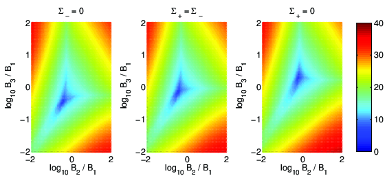
Figure 1: The convergence time for different initial values of $\mathcal{B}_{2}/\mathcal{B}_{1}$ and $\mathcal{B}_{3}/\mathcal{B}_{1}$. From left to right, the initial shear variables are taken to be $(\Sigma_{+},\Sigma_{-})=(\sqrt{0.2},0),(\sqrt{0.1},\sqrt{0.1}),(0,\sqrt{0.2})$. The other conditions are explained in the body of the text. There is no significant dependence on initial $\Sigma_{+}/\Sigma_{-}$. The typical convergence time appears to be between $10$ and $20$. While anisotropic phase lasts longer when the ratios between the magnetic components are extreme, note that the single component configuration $\mathcal{B}_{2}\sim\mathcal{B}_{3}\ll\mathcal{B}_{1}$ (left-bottom corners in the plots) is not efficient to generate anisotropy.

Figure 1 shows the colour-coded plot of the time $\tau$ (e-folding number) that elapsed before settling down to the isotropic magnetic inflation (convergence time). The initial ratios of $\mathcal{B}_{2},\mathcal{B}_{3}$ to $\mathcal{B}_{1}$ have been swept from $10^{-2}$ to $10^{2}$ while keeping fixed the other initial conditions as

$$\Sigma^{2}=\frac{1}{6}\varpi^{2}=\Omega_{V}=\Omega_{E}=\Omega_{B}=0.2\ .$$ (4.3)

The directions of electric field components are taken to be isotropic, namely

$$\mathcal{E}_{1}=\mathcal{E}_{2}=\mathcal{E}_{3}$$ (4.4)

and the three panels correspond to three representative choices of the direction of initial anisotropy

$$\Sigma_{-}=0\ ,\quad\Sigma_{+}=\Sigma_{-}\ ,\quad\Sigma_{+}=0\ .$$ (4.5)

In practice, one needs to specify the criterion for convergence since an orbit never reaches the attractor exactly, but only approaches to it asymptotically. Our choice is

$$|\Sigma_{+}|,|\Sigma_{-}|<10^{-3}\ ,\quad\left|\varpi-\frac{4}{\alpha+\lambda}\right|,\left|\Omega_{V}-\frac{3\lambda(\alpha+\lambda)+4}{3(\alpha+\lambda)^{2}}\right|<10^{-2}\ .$$ (4.6)

The latter two conditions are added to ensure that the isotropy is not accidental, but due to the convergence to the isotropic magnetic inflation.

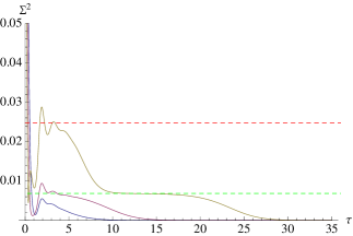
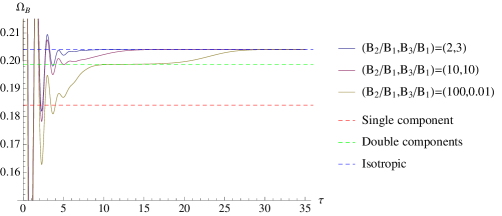
Figure 2: Transient anisotropy and convergence to the isotropic attractor. We plot the time evolution of $\Sigma^{2}$ and $\Omega_{B}$ for three initial magnetic configurations $(\mathcal{B}_{2}/\mathcal{B}_{1},\mathcal{B}_{3}/\mathcal{B}_{1})=(2,3),(10,10),(100,0.01)$. The shear variabels satisfy $\Sigma_{+}=\Sigma_{-}$ initially and the conditions are the same as specified in (4.3) and (4.4). The equilibrium values of $\Sigma^{2}$ and $\Omega_{B}$ at each of the inflationary fixed points are indicated by dotted lines. The maximum value of $\Sigma^{2}$ for $(B_{2}/B_{1},B_{3}/B_{1})=(10,10)$ roughly agrees with the equilibrium value of double component inflation. The orbit $(B_{2}/B_{1},B_{3}/B_{1})=(100,0.01)$ exhibits an intermediate stationary period at double component inflation and also a hint of initial attraction to single component inflation. While saddle behaviour is not so clear in $(B_{2}/B_{1},B_{3}/B_{1})=(2,3)$, it appears reasonable to attribute the initial anisotropic period to a temporal approach to anisotropic fixed point.

They show a clear tendency that a strong initial anisotropy in the configuration of magnetic field results in a prolonged period of anisotropic phase before the universe reaches the isotropic inflation (figure 2). When the initial magnetic components are of the same order (blue regions in figure 1), the typical time-scale of convergence to the attractor appears to be of order $\tau\sim 10$. This is much longer than the case of single scalar inflation where the typical convergence time is of order $\tau\sim 1$. Given that the extremum of anisotropy observed just before convergence agrees with the value of shear at the double magnetic fixed point (figure 2), it is reasonable to attribute the augmentation of convergence time to temporary attraction to those anisotropic solutions.

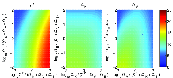
Figure 3: Left: color-coded plot of convergence time for varying $\Sigma^{2},\Omega_{B}$ and $\Omega_{K}=\Omega_{V}=\Omega_{E}$. The top-left corner corresponds to the initial universe dominated by magnetic sector and the bottom-right to shear domination. The dependence is rather weak (note the color scheme different from figure 1). Centre and right: similar plots for varying $\Omega_{K},\Omega_{B}$ and $\Omega_{V},\Omega_{B}$. The effect is even less significant.

Once the attraction occurs, it requires another $\sim O(10)$ e-foldings in order for becoming isotropic since the eigenvalues for instability of anisotropic inflation as well as stability of isotropic one are roughly proportional to the value of shear during the anisotropic phases, which is $\Sigma_{+}=-10/121$ for the double-component magnetic inflation with the current choice of the parameters.

Next, we study the dependence on the partition of the energy among different sectors while respecting the Friedmann equation (2.41). We fix the initial ratios between components of shear, electric and magnetic field as

$$\Sigma_{+}=\Sigma_{-}\ ,\quad\mathcal{E}_{1}=\mathcal{E}_{2}=\mathcal{E}_{3}\ ,\quad\mathcal{B}_{1}=\mathcal{B}_{2}=\mathcal{B}_{3}\ .$$ (4.7)

In the left panel of figure 3, we vary $\Omega_{B}/(\Omega_{K}+\Omega_{V}+\Omega_{E})$ and $\Sigma^{2}/(\Omega_{K}+\Omega_{V}+\Omega_{E})$ from $10^{-2}$ to $10^{2}$ while maintaining $\Omega_{K}=\Omega_{V}=\Omega_{E}$. Similar prescriptions for $\Omega_{B}$ - $\Omega_{K}$ and $\Omega_{B}$ - $\Omega_{V}$ have lead to the centre and right panels. It can be seen that the convergence time is rather insensitive to the total energy densities of each component (note the different color map from figure 1). The convergence time can be large for exceedingly large shear density, but otherwise it is about 10 e-foldings. While we have not presented any dependence on the directions and strengths of electric field, we mention that we checked their irrelevance in deciding the convergence as is expected from the general tendency to suppression of electric fields for $\lambda>0$.

4.2 Occurrence of oscillatory attractor in non-Abelian Bianchi I

Now we turn on the gauge coupling and repeat the same type of analysis as in the previous subsection. The figure 4 shows the convergence time for $\Gamma=0.1,0.5,1$ initially when the ratios $\mathcal{B}_{2}/\mathcal{B}_{1},\mathcal{B}_{3}/\mathcal{B}_{1}$ are varied under the same condition as in figure 1.

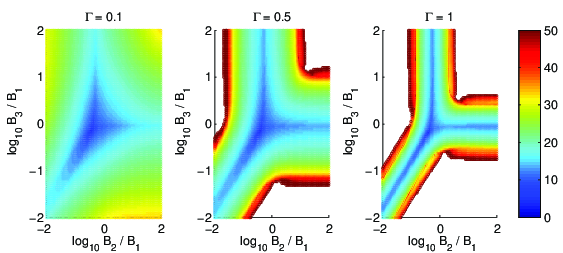
Figure 4: The same type of plots as the centre panel of figure 1 except that $\Gamma\neq 0$ initially here. The regions with long period of anisotropic inflation are now replaced by the oscillatory final state (white). Near the edge of the convergent area, the convergence time rises sharply. The larger is the initial value of $\Gamma$, the more often the system ends up in the oscillatory state.

First of all, one notices the sharp rise in convergence time when the initial magnetic configuration is anisotropic. Anisotropic phase may last more than 50 e-folds for $\Gamma=0.5$ or $1$ compared to 30 e-folds for $\Gamma=0$. Nevertheless, the final state is still the isotropic magnetic inflation and the dynamics is qualitatively similar to Abelian Bianchi I. On the contrary, in the white regions that are separated by those boundaries of prolonged anisotropic period, we have been unable to observe the convergence to the isotropic magnetic inflation. The dynamics in those regions is characterized by rapid oscillations of gauge field while the overall amplitudes of shear and gauge field energy density are decaying (figure 5). The period of oscillation decreases indefinitely so that the numerical calculations had to be abandoned typically around $\tau=10$. As one can see from figure 5, however, the system appears to settle down to a stationary state that is not a fixed point and dominated by the scalar field. The positive value of $q$ indicates that the expansion is no longer inflationary.

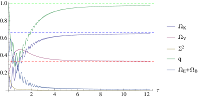
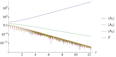
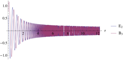
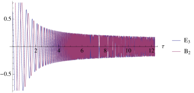
Figure 5: A typical oscillatory behaviour for $\alpha=2,\lambda=5$. The initial conditions are $\Sigma^{2}=\Omega_{K}=\Omega_{V}=\Omega_{E}=\Omega_{B}=0.2,\Omega_{N}=0,\Sigma_{+}=\Sigma_{-},\mathcal{E}_{3}=2\mathcal{E}_{1}=2\mathcal{E}_{2},\mathcal{B}_{2}=\mathcal{B}_{3}=100\mathcal{B}_{1}$. While not presented, $\mathcal{E}_{1}$ and $\mathcal{B}_{1}$ are exponentially suppressed. On the top-left panel, the values of $\Omega_{K},\Omega_{V}$ and $q$ for the power-law scalar solution (3.2) are indicated by the dotted lines with the corresponding colors.

Across those white regions, the dynamical behaviour shares several common features.

1. $\varpi,\Omega_{V}$ and $q$ appear to converge to constant values which are consistent with the conventional power-law fixed point by the scalar field (solution (3.2) which is not inflationary for $\alpha=2$). While $\Sigma_{+}^{2}+\Sigma_{-}^{2}$ and $\Omega_{E}+\Omega_{B}$ are also more or less constant, there contributions in the Friedmann equation and the other evolution equations for the isotropic variables (such as $\Omega_{K},\Omega_{V}$ and $q$) are subleading. Note, however, that it does not mean the final state is the fixed point (3.2) since it was already shown to be linearly unstable whence it cannot be an attractor.

2. There are always two components of electric as well as magnetic field that survive. The remaining one component for each decays exponentially. The three separated white regions correspond to three possible choices of two components out of three. The amplitudes of oscillation, and hence the expansion normalized energy density of gauge field, approach constant in the expanding universe with $q=1\Leftrightarrow p=1/2$, which means the gauge field is effectively behaving as a radiation fluid. This may be expected by observing that the structure of oscillation is similar to that of the familiar electromagnetic plane-wave.

3. For the vector potential $\mathcal{A}_{A}$, one component grows exponentially while the other two undergo oscillation damping. The growth of the single component is faster than the decay of $\Gamma$ (top-right panel in figure 5).

Given those observations, we look for an asymptotic oscillatory solution as follows. First, we assume the back reaction of gauge field on the scalar field dynamics is negligible and set $\varpi^{\prime}=\Omega_{V}^{\prime}=0$ in equations (2.54) and (2.55), obtaining

$$\varpi=\frac{2\left(q+1\right)}{\alpha}\ ,\quad\Omega_{V}=-\frac{2(q+1)(q-2)}{3\alpha^{2}}\ .$$ (4.8)

Further neglecting the effect of gauge field on the spacetime geometry, one effectively arrives at the scalar power-law solution (discussed in section 3.1)

$$q=\frac{\alpha^{2}-2}{2}\ .$$ (4.9)

Recall that this solution is not inflationary (namely $q>0$) if $\alpha>\sqrt{2}$. Second, assuming that $\mathcal{E}_{1}$ and $\mathcal{B}_{1}$ are decaying away, we solve the evolution equation for $\Gamma\mathcal{A}_{1}$ to yield

$$\Gamma\mathcal{A}_{1}=\Gamma(0)\mathcal{A}_{1}(0)e^{q\tau}\ .$$ (4.10)

Next, we use equations (2.51) - (2.53) and (2.57) - (2.59) to derive

$$\begin{split}&\mathcal{E}_{2}^{\prime}=\left[q-1-\frac{\lambda}{\alpha}(q+1)\right]\mathcal{E}_{2}+\Gamma\mathcal{A}_{1}\mathcal{B}_{3}\ ,\\ &\mathcal{B}_{3}^{\prime}=\left[q-1+\frac{\lambda}{\alpha}(q+1)\right]\mathcal{B}_{3}-\Gamma\mathcal{A}_{1}\mathcal{E}_{2}\ ,\end{split}$$ (4.11)

and an analogous set of equations for $\mathcal{E}_{3}$-$\mathcal{B}_{2}$. Because of the exponential growth of $\Gamma\mathcal{A}_{1}$ for $q>0$, the contribution from the first terms soon become negligible. The approximated solution is then given by

$$\mathcal{E}_{2}=C\sin\left(\frac{\Gamma(0)\mathcal{A}_{1}(0)}{q}e^{q\tau}+\phi_{0}\right)\ ,\quad\mathcal{B}_{3}=C\cos\left(\frac{\Gamma(0)\mathcal{A}_{1}(0)}{q}e^{q\tau}+\phi_{0}\right)\ .$$ (4.12)

The appearance of exponential growth inside the trigonometric functions explains the increasingly rapid oscillations towards the end and the numerical difficulty in that regime.

The fact that the spacetime evolution is effectively that of the power-law solution in section 3.1 might appear puzzling since that solution is linearly unstable for the current parameter set and thus cannot be an attractor. The linear analysis does not apply here, however, due to the prominent effect of $\Gamma\mathcal{A}_{1}$ terms in equations (4.11), which are higher order in perturbation. The net result of these terms is to force the gauge field to behave as an isotropic radiation fluid by making its components oscillate rapidly. Then, one might expect the fixed point (3.2) to effectively “become stable” since its only unstable modes come from the gauge field that now behaves as a radiation fluid. The power-law fixed point is stable against radiation fluid (and shear) as long as $\alpha\leq 2$ (in the case of equality it is marginally stable as we have seen here) so that this oscillatory regime can be an attractor.

It is observed that the condition for this oscillatory attractor to be reached is similar to that for a long anisotropic period in the Abelian Bianchi type I. In other words, the oscillation occurs when the components of magnetic fields have different magnitudes among them except for the configuration $\mathcal{B}_{2}\sim\mathcal{B}_{3}\ll\mathcal{B}_{1}$ and its permutations. It is reasonable considering the nature of the oscillation which requires two dominant components with one decaying exponentially. Although not presented here, the initial direction of shear does not play an important role in deciding the final state of the universe as in the Abelian case. The dependence on the initial value of $\Gamma$ is rather straightforward. The white regions start to appear around $\Gamma=0.3$ and grow larger as $\Gamma$ increases. The effect of unequal density parameters is investigated in figure 6. The convergence time is again mostly insensitive to them except for $\Sigma^{2}$, greater values of which induce oscillations even for isotropic initial magnetic field.

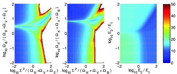
Figure 6: Left and centre: the convergence time for varying $\Sigma^{2}$ and $\Omega_{B}$ or $\Omega_{E}$. We have $\Sigma_{+}=\Sigma_{-}>0,\mathcal{E}_{1}=\mathcal{E}_{2}=\mathcal{E}_{3},\mathcal{B}_{1}=\mathcal{B}_{2}=\mathcal{B}_{3},\Gamma=1$ and $\Omega_{K}=\Omega_{V}=\Omega_{E}$ (or $=\Omega_{B}$). Again, $\Omega_{B}$ and $\Omega_{E}$ hardly influence the result while large $\Sigma^{2}$ drives oscillation even in the isotropic initial magnetic field. Right: the dependence on the initial direction of electric field. The initial condition is the equipartition (4.3) plus $\Sigma_{+}=\Sigma_{-}>0,\mathcal{B}_{1}=\mathcal{B}_{2}=\mathcal{B}_{3},\Gamma=1$. No significant dependence is seen.

5 The effect of spatial curvature

Now we are going to discuss how inclusion of spatial curvature changes the results obtained in the previous section. Again, $(\alpha,\lambda)=(2,5)$ is taken as the representative set of parameters. During inflation, spatial curvature is widely believed to be irrelevant. Although the local stability analysis supports this assumption, we will show that it does not apply to the global dynamics. In general, they tend to increase the time for convergence to the isotropic inflationary state, if it is asymptotically realized, and hence affect the physical predictions. It also drastically reduces the chance to encounter the oscillatory attractor.

5.1 Bianchi type II

The simplest spatially curved homogeneous model is Bianchi type II for which one of the $\mathcal{N}_{A}$’s is non-zero and the other two vanish. Without loss of generality, one can assume that the non-zero component is positive.

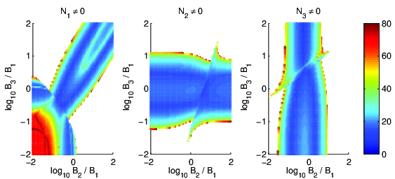
Figure 7: Dependence of convergence time on anisotropy in magnetic configuration for $\mathcal{N}_{1}\neq 0$, $\mathcal{N}_{2}\neq 0$ and $\mathcal{N}_{3}\neq 0$ respectively. The shapes of the contour are significantly different from the corresponding plot for type I (figure 4). When $\mathcal{N}_{1}\neq 0$, oscillation occurs for $\mathcal{B}_{2}\gg\mathcal{B}_{3}$ or $\mathcal{B}_{3}\gg\mathcal{B}_{2}$ and for corresponding cyclic permutations when $\mathcal{N}_{2}\neq 0$ or $\mathcal{N}_{3}\neq 0$. Also note that the anomalously long convergence time in the bottom-left corner of the left panel.

First of all, let us investigate the dependence on the anisotropy in the initial magnetic configuration, which turned out to be the deciding factor of the global dynamics for Bianchi type I. As for the initial data, we take all the density parameters to be equal

$$\Sigma^{2}=\Omega_{K}=\Omega_{V}=\Omega_{N}=\Omega_{E}=\Omega_{B}=\frac{1}{6}$$ (5.1)

and set

$$\Sigma_{+}=\Sigma_{-}\ ,\quad\mathcal{E}_{1}=\mathcal{E}_{2}=\mathcal{E}_{3}\ ,\quad\Gamma=1\ .$$ (5.2)

Figure 7 shows the convergence time for varying initial magnetic configuration with $\mathcal{N}_{1}\neq 0\,,\mathcal{N}_{2}\neq 0$ and $\mathcal{N}_{3}\neq 0$. The initial conditions for which the attractor is non-inflationary oscillatory solution are indicated by white as before. We see a significant change in the shape of white region compared to the corresponding plot for type I (right panel of figure 4). The three white regions in the Bianchi type I are reduced to two in the type II. A speculative interpretation is that the disappeared region corresponds to the single non-zero curvature component ($\mathcal{N}_{1}$ for the left panel and $\mathcal{N}_{2}$ for the centre). This means that the existence of spatial curvature prevents the system from evolving into the non-inflationary oscillatory solutions. This hypothesis is supported by the results for the other Bianchi types (See below for types VIII and IX, and Appendix for types VI₀ and VII₀.)

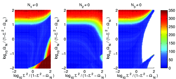
Figure 8: Dependence of the convergence time on initial amplitudes of $\Sigma^{2}$ and $\Omega_{N}$. The initial conditions satisfy $\Omega_{K}=\Omega_{V}=\Omega_{E}=\Omega_{B}$ and $\Sigma_{+}=\Sigma_{-}>0,\mathcal{E}_{1}=\mathcal{E}_{2}=\mathcal{E}_{3},\mathcal{B}_{1}=\mathcal{B}_{2}=\mathcal{B}_{3}$. The tendency towards a long period of anisotropic inflation is observed for large $\Omega_{N}$. The appearance of oscillation in $\mathcal{N}_{3}\neq 0$ for large $\Sigma^{2}$ is not totally surprising since the similar behaviour has been noted in type I, although the reason for its absence in $\mathcal{N}_{1}\neq 0$ and $\mathcal{N}_{2}\neq 0$ is unknown.

Figure 8 examines the effect of varying $\Omega_{N}$. Clearly, curvature-dominated universes undergo a particularly long period of anisotropic inflation, which may last more than $300$ e-foldings. Along with the left-bottom corner in the left panel of figure 7, such a prolonged anisotropic phase is not expected from the linear stability analysis. In any of those regions, the single-component phase appears to be responsible for the anisotropy as can be seen in figure 9. This is the topic of the next subsection.

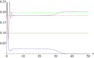
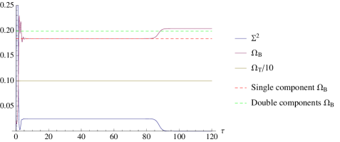
Figure 9: Transient anisotropy and convergence to the isotropic attractor for Bianchi type II. The initial conditions are; $\mathcal{N}_{1}\neq 0,\Sigma^{2}=\Omega_{K}=\Omega_{V}=\Omega_{N}=\Omega_{E}=\Omega_{B}=1/6,\mathcal{B}_{1}=10\mathcal{B}_{2}=10\mathcal{B}_{3}$ for left, $\mathcal{N}_{2}\neq 0,\Omega_{N}=9/10,\Sigma^{2}=\Omega_{K}=\Omega_{V}=\Omega_{E}=\Omega_{B}=1/50,\mathcal{B}_{1}=\mathcal{B}_{2}=\mathcal{B}_{3}$. The other conditions are as explained in the text. We also plot $\Omega_{T}$ to confirm that the Hamiltonian constraint is maintained. Both saddles are clearly seen in the right while the double component inflation is skipped in the left.

5.2 Quasi-single-component magnetic inflation

One may wonder why the anisotropic phases in type II (figure 9) could be as long as 100 e-folds while the stability analysis suggests that the linear instability kicks in after $\sim\Sigma^{-1}\sim 10$ e-folds. Although the values of $\Sigma^{2}$ and $\Omega_{B}$ during the anisotropic periods are almost exactly those for the single-component magnetic fixed point discussed in section 3.3.1, it turns out that the internal mechanism is very different, involving the spatial curvature.

Figure 10 shows time evolution of various quantities for the numerical solution presented in the right panel of figure 9.

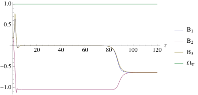
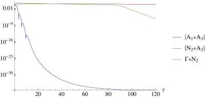
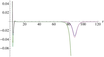
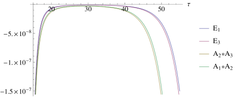
Figure 10: Dynamics for initial conditions $\mathcal{N}_{2}\neq 0,\Omega_{N}=9/10,\Sigma^{2}=\Omega_{K}=\Omega_{V}=\Omega_{E}=\Omega_{B}=1/50,\mathcal{B}_{1}=\mathcal{B}_{2}=\mathcal{B}_{3}$. Top-left: time evolution of magnetic components. Only $\mathcal{B}_{2}$ has a significant amplitude. Top-right: comparison between the two contributions to $\mathcal{B}_{2}$. The vertical axis is logarithmic. It is dominated by the curvature term. During the anisotropic phase, $\Gamma\mathcal{A}_{2}$ decays only slowly. Bottom: plots of $\mathcal{E}_{1},\mathcal{E}_{3},\mathcal{B}_{1},\mathcal{B}_{3}$ for different time-scales. Note that after $\tau\sim 90$, the electric components are exponentially suppressed.

From the top-left panel, the system experiences $\sim 80$ e-foldings of anisotropic inflation with non-vanishing $\mathcal{B}_{2}$. If this was the fixed point studied in section 3.3.1, $\mathcal{A}_{1}$ and $\mathcal{A}_{3}$ should be roughly constant during that period. But the top-right panel shows exponential decay of $\mathcal{A}_{1}\mathcal{A}_{3}$. Instead, $\mathcal{B}_{2}$ is dominated by the second term $-\mathcal{N}_{2}\mathcal{A}_{2}$ which involves the spatial curvature. According to this observation, one might suspect that there is another fixed point with non-vanishing $\mathcal{N}_{2}$ and constant $\mathcal{A}_{2}\mathcal{N}_{2}$ with exactly the same apparent behaviour. However, such a solution does not exist even asymptotically. In fact, one can see on the bottom-right that the other components of magnetic field ($\mathcal{B}_{1}=\mathcal{A}_{2}\mathcal{A}_{3}$ and $\mathcal{B}_{3}=\mathcal{A}_{1}\mathcal{A}_{2}$) as well as electric components do not behave as expected. If this could be understood by simple linear perturbation around a fixed point, the negligibly small $\mathcal{E}_{1},\mathcal{E}_{3},\mathcal{B}_{1}$ and $\mathcal{B}_{3}$ should have evolved monotonically (or oscillatory in case of imaginary eigenvalue) according to their stability. Here they all show both exponential decay and growth deep inside the period of the anisotropic inflation (between $\tau=10$ and $\tau=50$). In particular, the growth of electric components around $\tau=50$ is completely against the principle of magnetic inflation discussed so far.

This anomalous situation can be partially understood by taking a heuristic approach. First of all, let us assume that all the geometric and scalar-field variables take their equilibrium values for the single-component magnetic inflation. Further, from the numerical evidence, assume

$$\begin{split}&|\mathcal{B}_{1}|\gg|\mathcal{B}_{2}|\ ,\ |\mathcal{B}_{3}|\ ,\ |\mathcal{E}_{1}|\ ,\ |\mathcal{E}_{2}|\ ,\ |\mathcal{E}_{3}|\ ,\\ &|\mathcal{N}_{1}\mathcal{A}_{1}|\gg|\mathcal{A}_{2}\mathcal{A}_{3}|\ .\end{split}$$ (5.3)

Under these assumptions, we can derive the leading order behaviours

$$\mathcal{A}_{1}\propto e^{3\Sigma_{+}\tau}\ ,\quad\mathcal{N}_{1}\propto e^{-3\Sigma_{+}\tau}\ ,\quad\Gamma\propto e^{(q-\Sigma_{+})\tau}\ .$$ (5.4)

These indeed give the constant magnetic field $\mathcal{B}_{1}\sim-\mathcal{N}_{1}\mathcal{A}_{1}$. To see what happens to the other components of gauge field, we first note that

$$\Gamma\mathcal{A}_{1}\propto e^{(q+2\Sigma_{+})\tau}\ ,$$ (5.5)

with $0<\Sigma_{+},1+q\ll 1$ for realistic inflationary models. Hence this combination is always decaying with the exponent $|q+2\Sigma_{+}|\lesssim 1$ during the regime under consideration. The very slow decline as can be seen in figure 10 is expected to be rather peculiar for this set of parameters ($q+2\Sigma_{+}=-1/37$ for $\alpha=2,\lambda=5$). When it does happen, $\Gamma\mathcal{A}_{1}$ plays an important role in the evolution of the electromagnetic components perpendicular to $\mathcal{B}_{1}$. Their evolution equations can be evaluated as

$$\begin{split}\mathcal{E}_{2}^{\prime}\sim&\left(2q-2-\Sigma_{+}\right)\mathcal{E}_{2}+\Gamma\mathcal{A}_{1}\mathcal{B}_{3}\ ,\\ \mathcal{E}_{3}^{\prime}\sim&\left(2q-2-\Sigma_{+}\right)\mathcal{E}_{3}+\Gamma\mathcal{A}_{1}\mathcal{B}_{2}\ ,\\ \mathcal{B}_{2}^{\prime}\sim&3\Sigma_{+}\mathcal{B}_{2}-\Gamma\mathcal{A}_{1}\mathcal{E}_{3}\ ,\\ \mathcal{B}_{3}^{\prime}\sim&3\Sigma_{+}\mathcal{B}_{3}-\Gamma\mathcal{A}_{1}\mathcal{E}_{2}\ .\end{split}$$ (5.6)

Note that the mixing terms involving $\Gamma\mathcal{A}_{1}$ would have been by definition second order in perturbation for linear analysis in section 3.3.1. The dynamics of this coupled system crucially depends on the evolution of $\Gamma\mathcal{A}_{1}$, but the generic effect of the interaction terms is again oscillatory. This does not easily allow the magnetic components to grow indefinitely with the linear instability with respect to $\mathcal{B}_{1}$. At some stage, the present approximation breaks down ($\Gamma\mathcal{A}_{1}$ eventually dies away when $|q|>2\Sigma_{+}$) and the system leaves this regime. Numerical experiments suggest that this mechanism is in action whenever there appears an anisotropic inflationary period of much longer than $30$ e-folds. In more realistic models of inflation, however, since the decay of $\Gamma\mathcal{A}_{1}$ is expected to be much faster, the frequency of this event as well as the duration of anisotropic phase when it does occur should be much less than in our setup. This will be partially confirmed in section 6.

5.3 Generic Bianchi types

The most general anisotropic cosmologies are Bianchi type VIII and IX for which none of $\mathcal{N}_{A}$ vanishes. All the other types in class A can be considered as the boundary sets of these two (where behaviours can be very much different, see the Appendix for VI₀ and VII₀).

5.3.1 Bianchi type VIII

For type VIII, one can take one of $\mathcal{N}_{A}$ to be negative with the other two being positive, which implies positive definite $\Omega_{N}$.

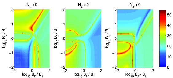
Figure 11: Plots of convergence time for varying magnetic field with different choices of negative $\mathcal{N}_{A}$. All the panels show qualitatively similar features. The convergence is fast for the region where $\mathcal{N}_{A}<0$ and $\mathcal{B}_{A}$ is greater compared to the other two magnetic components. As far as these blue regions are concerned, $\mathcal{N}_{2}<0$ and $\mathcal{N}_{3}<0$ are roughly symmetric in reflection with respect to the diagonal $\mathcal{B}_{2}=\mathcal{B}_{3}$. The slight skew is expected as $\Sigma_{-}\neq 0$ initially. Overall, the convergence appears to take longer than type I, probably because of the anisotropic nature of type VIII spatial curvature. No oscillation is observed in type VIII.

We repeat the same calculations as the type II with the initial conditions (5.1), (5.2) and the spatial curvature variables satisfying

$$|\mathcal{N}_{1}|=|\mathcal{N}_{2}|=|\mathcal{N}_{3}|\ .$$ (5.7)

Note that this configuration does not mean the spatial curvature is isotropic because of the differing signatures. The figure 11 shows plots for different choices of the negative component in spatial curvature. It is observed that the anisotropy is suppressed in the region where $\mathcal{B}_{A}$ is dominant over the other magnetic components for $\mathcal{N}_{A}<0$. For example, for the initial data with $\mathcal{N}_{1}<0$, the spacetime with $\mathcal{B}_{1}\gg\mathcal{B}_{2},\mathcal{B}_{3}$ will evolve rapidly into an isotropic one. This might be partially explained by the structure of the evolution equations of $\mathcal{E}_{1}$ and $\mathcal{B}_{1}$. The coupling between negative $\mathcal{N}_{1}$ and $\mathcal{B}_{1}$ drives $\mathcal{E}_{1}$ initially, which in turn accelerates the decay of $\mathcal{B}_{1}$ through $-\Gamma\mathcal{N}_{1}\mathcal{E}_{1}$.

In other areas, the anisotropic phase is typically longer than that in type I. No obvious connection can be seen between the initial anisotropy of magnetic components and the convergence time. Moreover, there is no oscillatory phase seen for type VIII even though $\Gamma=1$ initially.

5.3.2 Bianchi type IX

This subsection presents similar analysis for type IX for which $\mathcal{N}_{A}>0,A=1,2,3$. Since $\Omega_{N}$ is not necessarily positive here, the initial conditions have to be modified from (5.1). For left and right panels in figure 12, $\Omega_{N}$ is initially negative so that we take, for equipartition,

$$\Sigma^{2}=\Omega_{K}=\Omega_{V}=-\Omega_{N}=\Omega_{E}=\Omega_{B}=\frac{1}{4}\ .$$ (5.8)

The initial shear and electric field are fixed as before

$$\Sigma_{+}=\Sigma_{-}\ ,\quad\mathcal{E}_{1}=\mathcal{E}_{2}=\mathcal{E}_{3}\ .$$ (5.9)

Three different configurations of initial spatial curvature are studied:

$$\begin{split}{\rm Left}&:\mathcal{N}_{1}=\mathcal{N}_{2}=\mathcal{N}_{3}\ ,\\ {\rm Centre}&:\mathcal{N}_{1}=10\mathcal{N}_{2}=10\mathcal{N}_{3}\ ,\\ {\rm Right}&:10\mathcal{N}_{1}=\mathcal{N}_{2}=\mathcal{N}_{3}\ .\end{split}$$ (5.10)

$\Gamma=1$ is common to all of them. They appear qualitatively similar.

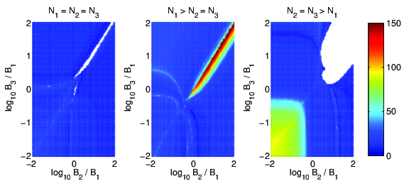
Figure 12: Plots of convergence time for varying magnetic field in type IX. Left: isotropic initial spatial curvature. The white strips represent the initial conditions that resulted in the recollapse of the universe. Unless it takes place, the final isotropic state is achieved within $15$-$20$ e-folds. Centre: $\mathcal{N}_{1}=10\mathcal{N}_{2}=10\mathcal{N}_{3}$ initially. Note that $\Omega_{N}>0$ in this case so that the equipartition condition is $\Sigma^{2}=\Omega_{K}=\Omega_{V}=\Omega_{N}=\Omega_{E}=\Omega_{B}=1/6$. In the red region, the intermediate evolution is the quasi-single-component magnetic inflation. Right: $10\mathcal{N}_{1}=\mathcal{N}_{2}=\mathcal{N}_{3}$. The white region is where the recollapse takes place.

The white regions in this case do not represent oscillation but the recollapse caused by growing negative $\Omega_{N}$ (figure 13). As far as we have checked, there is no oscillation observed for type IX either.

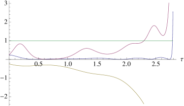
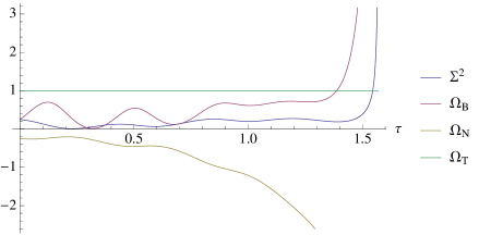
Figure 13: Two examples of recollapse taking place for type IX. The initial conditions are $\mathcal{N}_{1}=\mathcal{N}_{2}=\mathcal{N}_{3},\mathcal{B}_{2}=\mathcal{B}_{3}=10\mathcal{B}_{1}$ for left panel and $\mathcal{N}_{2}=\mathcal{N}_{3}=10\mathcal{N}_{1},\mathcal{B}_{2}=\mathcal{B}_{3}=10\mathcal{B}_{1}$ for right panel (each corresponding to a point in the white region of left and right panels in figure 12 respectively). One can observe that the density parameters blow up, in particular $\Omega_{N}$ goes negative, which indicates $H\rightarrow 0$. $\Omega_{T}$ is plotted to confirm that the calculation is not ruined by the rapidly changing variables.

For the isotropic spatial curvature, the convergence time is significantly shorter than type VIII. Notice that the spatial curvature for type VIII is anisotropic in nature. When curvature is anisotropic in type IX, the order of magnitude of convergence time is similar to type VIII indeed. In the strip along the line $\mathcal{B}_{2}=\mathcal{B}_{3}$ in the centre panel and the bottom-left region in the right panel, where convergence time is anomalously elongated, we confirmed that the anisotropic phase is given by the quasi-single-component magnetic inflation. It appears reasonable to conclude that the appearance of this phase is sensitive to the initial anisotropy in the spatial curvature but not the initial shear.

5.4 Relation between oscillation and spatial curvature

The numerical calculations suggest that spatial curvature generally suppresses occurrence of the oscillatory attractor. As an effort to identify the mechanism, let us look at the behaviour of the curvature variables $\mathcal{N}_{A}$ in the asymptotic oscillatory solution derived in the previous section. From equations (2.45) - (2.47), one can see

$$\mathcal{N}_{A}^{\prime}=\frac{1}{2}\left(q-1+\frac{\lambda}{2}\varpi\right)\mathcal{N}_{A}\rightarrow\mathcal{N}_{A}\sim\mathcal{N}_{A}(0)\exp\frac{(\alpha+\lambda)q+(\lambda-\alpha)}{2\alpha}\tau\ ,$$ (5.11)

where we used the condition of the power-law “fixed point” (4.8). Given $q>0$ and $\lambda>\alpha>0$, the exponent is positive so that $\mathcal{N}_{A}$ are all growing. The physically relevant variables $N_{A}=\Gamma\mathcal{N}_{A}$ go as $\propto e^{q\tau}$ as well so that the oscillatory regime is unstable against perturbations of spatial curvature.

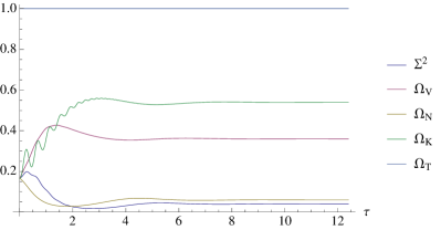
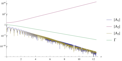
Figure 14: Left: behaviour of the density parameters during type II oscillation. Note the significant contribution of $\Sigma^{2}$ and $\Omega_{N}$ in contrast to the type I case. Right: time evolution of $\Gamma$ and components of vector potential for the same numerical solution. The apparent discontinuity in the oscillating vector potential is due to the logarithmic scale. The non-zero curvature component is $\mathcal{N}_{1}$ and the initial conditions are $\mathcal{B}_{2}=0.1\mathcal{B}_{1},\mathcal{B}_{3}=10^{3/2}\mathcal{B}_{1}$.

As the result, the oscillatory phases observed in type II (also IV₀ and VII₀) are in fact of a different nature from those in type I. Figure 14 shows what is going on when oscillation takes place in Bianchi type II. We see that the system appears to settle down to stationary attractor state before the Hamiltonian constraint breaks down due to numerical difficulty caused by rapid oscillation. The difference from type I (figure 5) is the non-vanishing energy density of shear and curvature. The vector potential appears to have the same feature of one growing and two damped oscillation components. To find the asymptotic type II solution similar to (4.12), we assume $\mathcal{N}_{1}\neq 0,\Sigma_{-}=0$ and set $\Sigma_{+},\varpi,\Omega_{V},\Omega_{N}=\Gamma^{2}\mathcal{N}_{1}^{2}/12$ all to be constant. From the equilibrium conditions, we derive

$$\begin{split}&q=4\Sigma_{+}\ ,\quad\Gamma^{2}\mathcal{N}_{1}^{2}=6\Sigma_{+}(2\Sigma_{+}-1)\ ,\quad\varpi=\frac{2}{\alpha}\left(4\Sigma_{+}+1\right)\ ,\\ &\Omega_{V}=-\frac{4}{3\alpha^{2}}\left(4\Sigma_{+}+1\right)\left(2\Sigma_{+}-1\right)\ .\end{split}$$ (5.12)

Note that $\Sigma_{+}$ has to be positive in order for $\Omega_{V}>0$. Now the solution for equation (2.56) is

$$\Gamma\sim\Gamma(0)\exp\left(\frac{\alpha-\lambda}{2\alpha}(4\Sigma_{+}+1)\tau\right)$$ (5.13)

which is consistent with exponential decay seen in figure 14 for $\lambda>\alpha$. Let us assume that the oscillation occurs within 1- and 3-components of electric and magnetic fields and the 2-components die away. One can then solve the evolution equation for $\mathcal{A}_{2}$ (2.49) to obtain

$$\Gamma\mathcal{A}_{2}\sim\Gamma(0)\mathcal{A}_{2}(0)e^{3\Sigma_{+}\tau}\ ,$$ (5.14)

which indicates the exponential growth of $\mathcal{A}_{2}$. Analogous to type I, the evolution equations for the oscillatory components are

$$\begin{split}\mathcal{E}_{1}^{\prime}=&\left[2\Sigma_{+}-1-\frac{\lambda}{\alpha}\left(4\Sigma_{+}+1\right)\right]\mathcal{E}_{1}-\Gamma\mathcal{N}_{1}\mathcal{B}_{1}+\Gamma(0)\mathcal{A}_{2}(0)e^{3\Sigma_{+}\tau}\mathcal{B}_{3}\ ,\\ \mathcal{B}_{3}^{\prime}=&\left[5\Sigma_{+}-1+\frac{\lambda}{\alpha}\left(4\Sigma_{+}+1\right)\right]\mathcal{B}_{3}-\Gamma(0)\mathcal{A}_{2}(0)e^{3\Sigma_{+}\tau}\mathcal{E}_{1}\ ,\end{split}$$ (5.15)

with a corresponding set of equations for $\mathcal{E}_{3}$ and $\mathcal{B}_{1}$. Recalling $\Gamma\mathcal{N}_{1}$ is constant, the exponential electromagnetic mixing terms soon dominate the dynamics and we obtain the asymptotic solution

$$\mathcal{E}_{1}=C\sin\left(\frac{\Gamma(0)\mathcal{A}_{2}(0)}{3\Sigma_{+}}e^{3\Sigma_{+}\tau}+\phi_{0}\right)\ ,\quad\mathcal{B}_{3}=C\cos\left(\frac{\Gamma(0)\mathcal{A}_{2}(0)}{3\Sigma_{+}}e^{3\Sigma_{+}\tau}+\phi_{0}\right)\ .$$ (5.16)

The same construction works for assumption of growing $\mathcal{A}_{3}$, leading to oscillation of $\mathcal{E}_{1},\mathcal{B}_{2}$ and $\mathcal{E}_{2},\mathcal{B}_{1}$. However, growing $\mathcal{A}_{1}$ and decaying $\mathcal{A}_{2},\mathcal{A}_{3}$ are not compatible with decaying $\mathcal{E}_{1}$ and $\mathcal{B}_{1}$. It is due to the definition of magnetic field

$$\mathcal{B}_{1}=\mathcal{A}_{2}\mathcal{A}_{3}-\mathcal{N}_{1}\mathcal{A}_{1}\rightarrow-\mathcal{N}_{1}(0)\Gamma(0)\frac{\mathcal{A}_{1}}{\Gamma}\ ,$$ (5.17)

which implies $\mathcal{B}_{1}$ should be rapidly growing instead of oscillating. Hence, the spatial curvature in 1-direction $\mathcal{N}_{1}$ kills the possibility of oscillation in 2- and 3-components of electromagnetic field. This explains the disappearance of the white region for regime $\mathcal{B}_{2}\sim\mathcal{B}_{3}\gg\mathcal{B}_{1}$ in the left panel of figure 7 that existed in type I (figure 4) since the oscillation in the region is precisely that among 2- and 3-components as observed in figure 5. Note that the asymptotic solution given by (5.12) and (5.16) is again unstable against perturbation of $N_{2}$ and $N_{3}$. Therefore, one can further speculate that the absence of oscillation in type VIII and type IX is indeed attributed to the presence of spatial curvature. To consolidate this conclusion, it would be ideal to perform similar numerical calculations for models with two non-vanishing components of spatial curvature, namely type VI₀ and VII₀. Unfortunately, it turns out to be impossible for the initial data with the equipartition condition such as (5.1) because of a technical problem, which is explained and alleviated in the Appendix. The modified analysis there indeed suggests that our conclusion is plausible.

6 Dependence on the parameters $\alpha$ and $\lambda$

So far, all the numerical results presented have been obtained for a particular parameter set $(\alpha,\lambda)=(2,5)$. As already explained, the reason for the choice is mostly the convenience and clarity. In reality, one would have liked to have a smaller slow-roll parameter $\epsilon=q+1$. In this section, we demonstrate that the qualitative features are more or less invariant against changes in $\alpha$ and $\lambda$ while the quantitative ones can vary according to $\epsilon$. In particular, we find the general tendency that smaller $\epsilon$ results in longer anisotropic period before the convergence to the final attractor.

6.1 Strength of the stability of the isotropic magnetic inflation

In the previous section, we saw that the typical convergence time for $(\alpha,\lambda)=(2,5)$ is of order $10$ e-foldings, except when the curvature-driven single component magnetic inflation stretches the anisotropic period. We argued that this order is determined by the magnitude of eigenvalues that determine the instability of anisotropic inflations as well as the stability of isotropic solution. To test our hypothesis, further numerical calculations have been carried out for six different parameter sets: $(\alpha,\lambda)=(2,5),(2,10),(2,50),(3,10),(1,5)$, and $(1,3)$. $(2,10)$ and $(2,50)$ have been chosen to demonstrate the dependence on the slow-roll parameter ($\epsilon=1/3,1/13$ respectively). $(3,10)$ is expected to exhibit a similar behaviour as $(2,5)$ and $(1,5)$ is supposed to provide a representative result for the situation where the scalar field by itself is capable of accelerated expansion ($\alpha<\sqrt{2}$). The last set $(1,3)$ is a critical value at which $\Omega_{B}$ evaluated at the isotropic magnetic inflation becomes zero and it merges with the conventional power-law fixed point. When $\alpha<1,\lambda<3$, the usual cosmic-no-hair holds and the convergence should be very rapid. This merginal case is included here to give a flavor of that transition. We have taken the initial conditions

$$\begin{split}&\Sigma_{+}=\Sigma_{-}=\sqrt{0.1}\ ,\quad\mathcal{N}_{1}=\mathcal{N}_{2}=\mathcal{N}_{3}=0\ ,\quad\Gamma=0.01\\ &\mathcal{E}_{1}=\mathcal{E}_{2}=\mathcal{E}_{3}=\sqrt{0.4}\ ,\quad\varpi=\sqrt{1.2}\ ,\quad\Omega_{V}=0.2\ ,\end{split}$$ (6.1)

and varied the magnetic components as

$$\frac{\mathcal{B}_{2}}{\mathcal{B}_{1}},\frac{\mathcal{B}_{3}}{\mathcal{B}_{1}}\in[10^{-2},10^{2}]\ ,\quad\Omega_{B}=0.2\$$ (6.2)

(the same prescription as the figure 1).

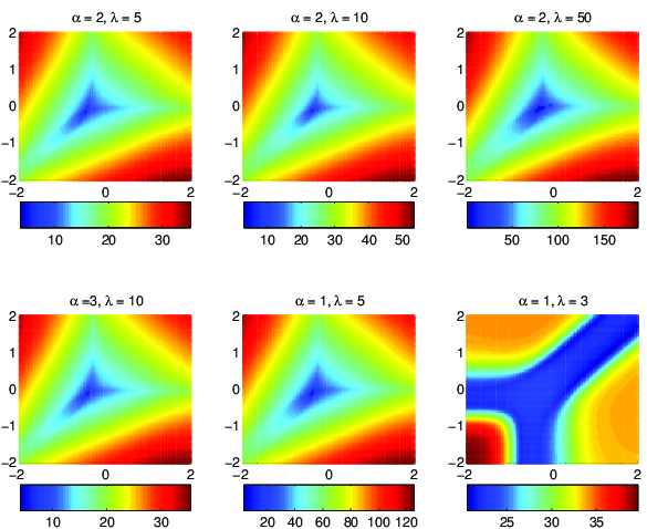
Figure 15: Parameter dependence of the convergence time for Bianchi type I with $\Gamma=0.01$ initially. The horizontal and vertical axes represent ${\rm log}_{10}\mathcal{B}_{2}/\mathcal{B}_{1}$ and ${\rm log}_{10}\mathcal{B}_{3}/\mathcal{B}_{1}$ respectively. Note the different color codings for different sets of parameters. As expected, the convergence for $(1,3)$ is fast and insensitive to the initial direction of magnetic field.

At a glance, the results (figure 15) look identical for all the parameter sets but $(\alpha,\lambda)=(1,3)$ for which we should see a qualitatively different behaviour (the gauge field actually vanishes in the final state). Even though the patterns are identical, however, the different color maps mean the time-scales of convergence vary significantly.

According to the linear stability analysis in section 3, the convergence time should be related to the values of $\Sigma_{+}$ for single- and double-component magnetic inflations.

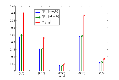
Figure 16: Parameter dependence of the eigenvalues characterizing different magnetic inflations. The associated time-scales are determined as the inverse of these values. They agree with the results in figure 15 well.

In figure 16, we plotted the characteristic eigenvalues for single-component, double-component and isotropic magnetic inflations. As already noted, the time-scales determined by these eigenvalues are all similar for each given parameter set. The values read off from the graph explain the results of numerical calculations well. For instance, $(2,10)$ takes twice as much time as $(2,5)$, $(2,5)$ and $(3,10)$ should have similar convergence time, and so on.

To see the relation between the convergence time and the slow-roll parameter $\epsilon$, we note that for an acceptable inflationary model, $\epsilon$ must be sufficiently small, i.e.,

$$\epsilon=q+1=\frac{2\alpha}{\alpha+\lambda}\ll 1,$$ (6.3)

which is roughy equivalent to $\alpha\ll\lambda$. Using this approximation, one can see

$$\Sigma_{+}\big{|}_{\rm single\mathchar 45\relax comp}\sim\frac{\alpha\lambda-4}{3\lambda^{2}+8}\ ,\quad\Sigma_{+}\big{|}_{\rm double\mathchar 45\relax comp}\sim\frac{\alpha\lambda-4}{3\lambda^{2}+2}\ .$$ (6.4)

Therefore, the characteristic time-scale should be at least

$$\tau_{c}\gtrsim\frac{3\lambda^{2}}{\alpha\lambda-4}>\frac{3\lambda}{\alpha}\sim 6\epsilon^{-1}\ .$$ (6.5)

This implies that we should expect an anisotropic phase of order $\epsilon^{-1}$ at least. This will be an accurate estimate if $\alpha\lambda\gg 4$. On top of this generic lower bound, anisotropic phase should be further extended if $\alpha\lambda\sim 4$, which is exactly when $\Sigma_{+}$ become very small. Given the observationally favored value $\epsilon\lesssim 10^{-2}$ [70], it appears unlikely to see the convergence to the isotropic attractor before $100$ e-foldings. From another point of view, even when multiple gauge fields are present, the period of anisotropic inflation may well be observable and tightly constrained.

6.2 Effect on the oscillatory phase

Figure 17 shows the convergence time in non-Abelian Bianchi I ($\Gamma=1$ initially) for the different parameter sets.

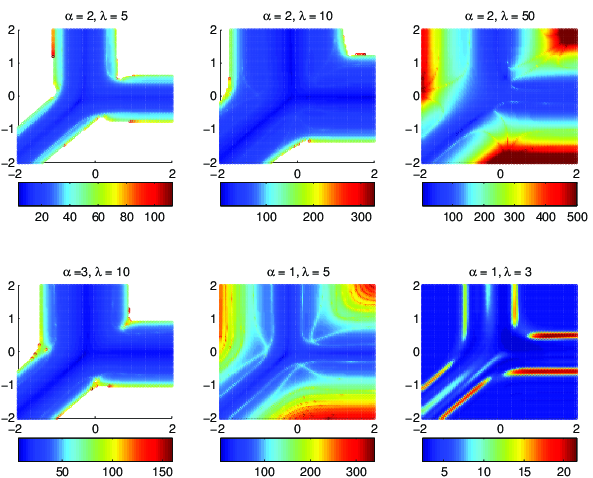
Figure 17: Parameter dependence of non-Abelian ($\Gamma=1$) Bianchi I. The initial conditions are the same as in figure 15 except for $\Gamma$. The axes are again directions of magnetic components.

The absence of the oscillatory phase for $\alpha=1$ is noted. It is expected since the exponential growth in equations (4.10) and (4.11) happens only if $q$ is positive while it should be negative for $\alpha<\sqrt{2}$. This leads to an interesting result that if the scalar field is capable of accelerated expansion by itself, there will be no oscillation after introducing gauge fields. The area of oscillation seems to be squeezed for greater $\lambda$ even for $\alpha=2$ and almost disappears when $\lambda=50$. Although the reason is not clear, we suspect that it is due to the back reaction of the gauge field onto the scalar field through equation (2.54) where its effect is amplified by the factor of $\lambda$.

We also find the oscillation for $\alpha=3$. Since the isotropic fixed point (3.2) is physically admissible only for $\alpha\leq\sqrt{6}$, this oscillating solution does not correspond to the fixed point. In fact, the asymptotic state of the universe here is anisotropic. The nature of oscillation is rather akin to that of Bianchi type II. The energy density of shear as well as gauge field cannot be ignored and settles down to a constant final value.

6.3 Suppression of the anomalously long anisotropic phase

In the discussion of the prolonged anisotropic phases encountered in the presence of spatial curvature, we mentioned that this would be a peculiar feature for the specific parameter values $(\alpha,\lambda)=(2,5)$.

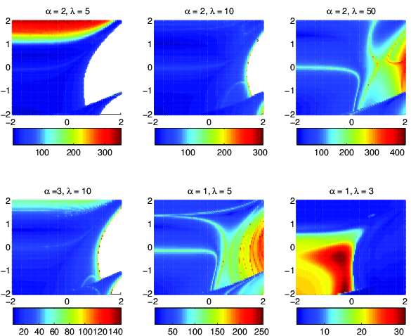
Figure 18: Convergence time in type II ($\mathcal{N}_{3}\neq 0$) for the different parameter sets under varying density parameters. The initial conditions are $\Omega_{K}=\Omega_{V}=\Omega_{E}=\Omega_{B},\Sigma_{+}=\Sigma_{-},\mathcal{E}_{1}=\mathcal{E}_{2}=\mathcal{E}_{3},\mathcal{B}_{1}=\mathcal{B}_{2}=\mathcal{B}_{3}$ and $\Gamma=1$. The x-axes; $\Sigma^{2}/\left(1-\Sigma^{2}-\Omega_{N}\right)$. The y-axes; $\Omega_{N}/\left(1-\Sigma^{2}-\Omega_{N}\right)$.

Figure 18 duly confirms our statement. Aside from the top-left panel, the typical convergence time agrees with the one estimated from the eigenvalues, and with the figure 15. In all the cases from figure 15 to 18, the contour patterns are very similar for different parameters. This implies that the qualitative behaviours for $(\alpha,\lambda)=(2,5)$ studied in detail in the present paper are generic.

7 Concluding remarks

In this article, we studied a general class of anisotropic cosmological models that contain a scalar field with exponential potential and an SU(2) gauge field coupled to the scalar through exponential gauge-kinetic function. The governing equations have been properly normalized so that all the important inflationary solutions appear as fixed points of the dynamical system. We carried out the detailed stability analysis for them and have explicitly confirmed that the only stable attractor solution is the isotropic magnetic inflation. The peculiarity arising from the Yang-Mills interaction and spatial curvature has also been pointed out, which differentiates this model from the more regular U(1) triplet system. Then, extensive numerical investigations have been made to survey a variety of initial conditions and to see how convergence to the stable isotropic solution with magnetic field is achieved. We found several different types of oscillatory attractors that prevent the universe from settling down to the isotropic inflation. The inclusion of fully generic spatial curvature (type VIII and type IX) has been shown to restore the stability of inflation globally. Nevertheless, the time it takes for the anisotropy to disappear is rather significant, at the very least $10$ e-foldings. This estimate agrees with the characteristic eigenvalues of the isotropic as well as anisotropic inflationary solutions and we have obtained the general lower bound for convergence time in terms of the slow-roll parameter, namely $\tau_{c}\gtrsim\epsilon^{-1}$. In summary, it is reasonable to conclude that the isotropic magnetic inflation is stable for a large class of initial conditions in the general homogeneous cosmologies. From a physical point of view, however, it is very likely that we should see the signature of transient anisotropy, which may well last until the end of inflation.

Although we have revealed new interesting properties of anisotropic inflation in the theory with gauge-kinetic coupling, this model may not be realistic due to the idealized and simplified choice of the action. The resent observational data rejects a power-law inflation model [70]. It should also be pointed out that the inflation is inherently eternal in the present model because the exponential potential and gauge-kinetic coupling are scale-free so that there is the problem of graceful exit. An obvious next step will be to study the effects of the gauge-kinetic term on more realistic inflationary models based on fundamental unified theories such as superstring theory, for example, brane inflation[71, 72, 13, 14] or higher-order curvature inflation [73, 74, 75, 76, 77, 78, 53]. We should also find a way out of the accelerated expansion in those models and provide a concrete example of successful reheating after inflation.

From a phenomenological point of view, the relevance of inflaton-gauge interaction in the context of statistical anisotropy in CMBR is made more interesting by our finding that anisotropic inflation is quite generic as far as our observational window of around 60 e-foldings is concerned even though the mathematically defined attractor is isotropic. Quantitative estimates of CMBR anisotropy generated by the transient anisotropic phase and its scale-dependence caused by the transition from anisotropic phase to isotropic one may deserve more serious attention. These studies are left for future projects.

Appendix A Abelian dynamics

In this section, we discuss the formulation of the problem in the case of three Abelian gauge fields and present some numerical results for the purpose of comparison. Let us assume the condition (2.32) and fix the frame such that all the anisotropic variables are diagonal. First of all, we note that the vector potential completely disappears from equations by setting $g=0$ in (2.17), (2.18), (2.27) and (2.28). Hence, we do not need normalized variables $\mathcal{A}_{A}$ and $\Gamma$. Using the standard normalization (2.34) and

$$\mathcal{E}_{A}=\frac{e^{\lambda\varphi/2}E_{A}}{H}\ ,\quad\mathcal{B}_{A}=\frac{e^{\lambda\varphi/2}B_{A}}{H}\ ,$$ (A.1)

the Maxwell’s equations are given as

$$\begin{split}\mathcal{E}_{1}^{\prime}=&\left(q-1-\frac{\lambda}{2}\varpi-2\Sigma_{+}\right)\mathcal{E}_{1}-N_{1}\mathcal{B}_{1}\ ,\\ \mathcal{E}_{2}^{\prime}=&\left(q-1-\frac{\lambda}{2}\varpi+\Sigma_{+}+\sqrt{3}\Sigma_{-}\right)\mathcal{E}_{2}-N_{2}\mathcal{B}_{2}\ ,\\ \mathcal{E}_{3}^{\prime}=&\left(q-1-\frac{\lambda}{2}\varpi+\Sigma_{+}-\sqrt{3}\Sigma_{-}\right)\mathcal{E}_{3}-N_{3}\mathcal{B}_{3}\ ,\\ \mathcal{B}_{1}^{\prime}=&\left(q-1+\frac{\lambda}{2}\varpi-2\Sigma_{+}\right)\mathcal{B}_{1}+N_{1}\mathcal{E}_{1}\ ,\\ \mathcal{B}_{2}^{\prime}=&\left(q-1+\frac{\lambda}{2}\varpi+\Sigma_{+}+\sqrt{3}\Sigma_{-}\right)\mathcal{B}_{2}+N_{2}\mathcal{E}_{2}\ ,\\ \mathcal{B}_{3}^{\prime}=&\left(q-1+\frac{\lambda}{2}\varpi+\Sigma_{+}-\sqrt{3}\Sigma_{-}\right)\mathcal{B}_{3}+N_{3}\mathcal{E}_{3}\ ,\end{split}$$ (A.2)

with the spatial curvature variables satisfying

$$\begin{split}N_{1}^{\prime}=&(q-4\Sigma_{+})N_{1}\ ,\\ N_{2}^{\prime}=&(q+2\Sigma_{+}+2\sqrt{3}\Sigma_{-})N_{2}\ ,\\ N_{3}^{\prime}=&(q+2\Sigma_{+}-2\sqrt{3}\Sigma_{-})N_{3}\ .\end{split}$$ (A.3)

For the other equations, one only has to replace $\Gamma\mathcal{N}_{A}$ by $N_{A}$. Note that the magnetic fields $\mathcal{B}_{A}$ do not appear from the vector potential as long as it is assumed to be homogeneous.

One can confirm that the type I invariant set $N_{A}=0$ coincides with what we called Abelian boundary $\Gamma=0$ in the dynamical system discussed in the main body of the article.

The Abelian system behaves much better than the non-Abelian one. For instance, the double-component magnetic inflation is a usual fixed point and for the case of $\mathcal{B}_{1}=0$, the eigenvalues are given by

$$\begin{split}&\omega_{\Sigma_{+}-\varpi-\Omega_{B}}=\frac{q-2\pm\sqrt{\left(q-2\right)^{2}+12\Omega_{B}\left(\lambda\left(\alpha+\lambda\right)-2\right)}}{2}\ ,\\ &\omega_{\Sigma_{+}-\varpi}=q-2\ ,\quad\omega_{\Sigma_{-}-\mathcal{B}_{-}}=\frac{q-2\pm\sqrt{\left(q-2\right)^{2}-24\Omega_{B}}}{2}\ ,\\ &\omega_{N_{1}}=3\frac{2\alpha^{2}+2\alpha\lambda-\lambda^{2}-6}{(\alpha+\lambda)(\alpha+3\lambda)+2}\ ,\quad\omega_{N_{2}}=\omega_{N_{3}}=-3\frac{\lambda^{2}-2}{(\alpha+\lambda)(\alpha+3\lambda)+2}\ ,\\ &\omega_{\mathcal{B}_{1}}=-3\Sigma_{+}\ ,\quad\omega_{\mathcal{E}_{1}}=3\frac{\alpha^{2}-\alpha\lambda-4\lambda^{2}-4}{(\alpha+\lambda)(\alpha+3\lambda)+2}\ ,\quad\omega_{\mathcal{E}_{2}}=\omega_{\mathcal{E}_{3}}=\frac{-6\lambda(\alpha+2\lambda)}{(\alpha+\lambda)(\alpha+3\lambda)+2}\ ,\end{split}$$ (A.4)

which confirms that all the eigenvalues except for $\omega_{\mathcal{B}_{1}}$ possess negative real part provided that $\lambda$ is sufficiently greater than unity.

Figures 19 and 20 show how initial magnetic configuration affects the convergence time for Abelian case.

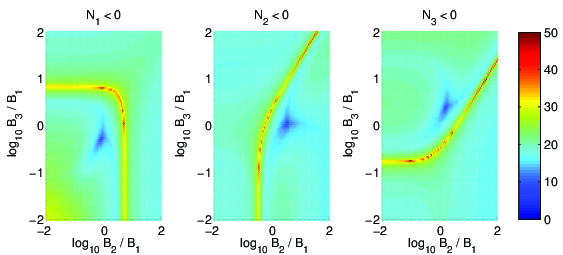
Figure 19: Dependence of convergence time on initial magnetic configuration for Abelian Bianchi type VIII. Each panel should be compared with the corresponding one in figure 11. While red contours are clearly identified between Abelian and non-Abelian plots, the latter exhibits more complicated patterns and longer anisotropic period.

As before, our initial conditions are taken to be equipartition of energy (either (5.1) or (5.8) depending on the signature of $\Omega_{N}$) and $\Sigma_{+}=\Sigma_{-},\mathcal{E}_{1}=\mathcal{E}_{2}=\mathcal{E}_{3}$. For type VIII, three different choices of the negative spatial curvature component with (5.7) are taken. For type IX, we have tried the isotropic initial curvature as well as two different preferred directions.

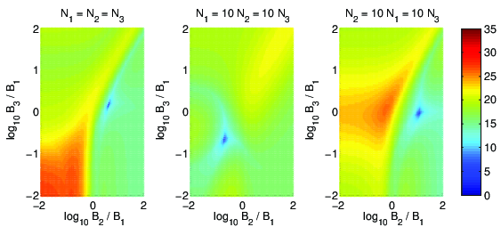
Figure 20: Convergence time for Abelian Bianchi type IX. The left and center panels have counterparts in the left and center of figure 12 respectively. For Abelian models, anisotropic type IX curvature does not extend period of anisotropic inflation significantly.

Comparing these with figures 11 and 12, overall patterns look similar for type III while the absence of the recollapsing and anisotropic strips in type IX is noted. From the discussion in section 5.2, the enhancement of anisotropy should not happen in Abelian dynamics and the result confirms it.

Appendix B Alternative numerical results tailored for Bianchi type VI₀ and VII₀

When the rank of 3 by 3 matrix $n_{AB}$ is 2, the homogeneous spatial geometry is classified into type VI₀ or VII₀ according to $\lambda_{1}\lambda_{2}\gtrless 0$ where $\lambda_{1}$ and $\lambda_{2}$ are the two non-zero eigenvalues of $n_{AB}$. In the setup of the present article, one can assume $n_{1}>0,n_{2}<0$ for VI₀ and $n_{1}>0,n_{2}>0$ for VII₀ without loss of generality.

For the purpose of our numerical calculations, it is desirable to specify the initial conditions of $\mathcal{B}_{A}$ instead of $\mathcal{A}_{A}$ since the former give physical measure of dynamical contribution of magnetic components. However, $\mathcal{A}_{A}$’s being the fundamental variables in terms of which the actual equations have been written down, one has to solve (2.37) for $\mathcal{A}_{A}$’s to set the initial conditions for each given run of numerical calculation. In an attempt to generate a figure analogous to figure 7, let us assume that we are given non-zero values for $\mathcal{B}_{1},\mathcal{B}_{2},\mathcal{B}_{3},\mathcal{N}_{1},\mathcal{N}_{2}$ while $\mathcal{N}_{3}$ vanishes. Eliminating $\mathcal{A}_{2}$ and $\mathcal{A}_{3}$, one obtains a quartic equation for $\mathcal{A}_{1}$

$$\mathcal{N}_{1}\mathcal{A}_{1}^{4}+\mathcal{B}_{1}\mathcal{A}_{1}^{3}-\mathcal{B}_{2}\mathcal{B}_{3}\mathcal{A}_{1}-\mathcal{N}_{2}\mathcal{B}_{3}^{2}=0\ .$$ (B.1)

Since the highest power of $\mathcal{A}_{1}$ is even, this equation may not have a real root depending on the values of magnetic field and spatial curvature. At least a real root always exists for type II, VIII or IX since the resulting algebraic equation is either odd or proportional to $\mathcal{A}_{1}$. Since we are varying the ratios of magnetic components by a factor of $10^{4}$, the parameter regions in which no real root exists are encountered during the calculations and it is impossible to produce density plots that can be compared to figures 7, 11 and 12.

To circumvent this problem, we abandon the initial equipartition of energy and directly specify the components of vector potential $\mathcal{A}_{1},\mathcal{A}_{2},\mathcal{A}_{3}$. The primary goal of studying type VI₀ and VII₀ is to confirm that the oscillation of electric and magnetic fields occurs only on the plane perpendicular to the single direction for which the curvature is absent. Since we already saw that the varying initial energy densities for magnetic field or spatial curvature do not very much change the conditions for oscillation in the case of type I and II, we expect to see the aforementioned feature. Our setup for the numerical calculations is as follows. First of all, we fix the initial values of shear, electric field, scalar kinetic energy and $\Gamma$ as

$$\Sigma_{+}=\Sigma_{-}=\sqrt{0.1}\ ,\quad\mathcal{E}_{1}=\mathcal{E}_{2}=\mathcal{E}_{3}=\sqrt{0.4}\ ,\quad\varpi=\sqrt{1.2}\ ,\quad\Gamma=1\ .$$ (B.2)

Next, we choose the 2- and 3-components of magnetic field to be varied. The specific prescription is given by

$$\mathcal{A}_{2}\mathcal{A}_{3}=\frac{\sqrt{0.6}}{100}\ ,\quad\frac{\mathcal{A}_{1}}{\mathcal{A}_{2}},\frac{\mathcal{A}_{1}}{\mathcal{A}_{3}}\in\left[10^{-2},10^{2}\right]\ ,\quad\mathcal{A}_{1}>0\ ,\mathcal{A}_{2}>0\ ,\mathcal{A}_{3}>0\ .$$ (B.3)

Note that this corresponds to setting

$$\mathcal{B}_{1}=\frac{\sqrt{0.6}}{100}\ ,\quad\frac{\mathcal{B}_{2}}{\mathcal{B}_{1}},\frac{\mathcal{B}_{3}}{\mathcal{B}_{1}}\in\left[10^{-2},10^{2}\right]$$ (B.4)

for Bianchi type I, in which case $\Omega_{B}$ would vary between $\sim 10^{-4}$ and $\sim 0.2$. When the spatial curvature exists, the magnetic field receives extra contributions involving $\mathcal{N}_{A}$ and the condition $\Omega_{B}<0.4$ that is required by the Hamiltonian constraint and positivity of $\Omega_{V}$ with (B.2) is not guaranteed. To reduce the chance of breaching this upper bound, we fix the amplitude of each spatial curvature variable to be $|\mathcal{N}_{A}|=0.1$ whenever one is non-zero so that the modification to $\mathcal{B}_{A}$ is suppressed by a factor of $10$. This results in initial curvature density

$$\Omega_{N}=\begin{cases}1/12&({\rm type\ II})\ ,\\ 1/3&({\rm type\ VI}_{0})\ ,\\ 0&({\rm type\ VII}_{0})\ .\end{cases}$$ (B.5)

Finally, the scalar potential is determined by

$$\Omega_{V}=0.4-\Omega_{B}-\Omega_{N}$$ (B.6)

with its positivity being checked for each iteration. It turns out that the regions discarded due to a negative value of $\Omega_{V}$ are indiscernible in the following plots.

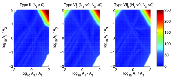
Figure 21: Dependence of convergence time on initial vector potential. We chose $\mathcal{N}_{1}>0$ for type II, $\mathcal{N}_{1}>0,\mathcal{N}_{2}<0$ for type VI₀ and $\mathcal{N}_{1}>0,\mathcal{N}_{2}>0$ for type VII₀. The disappearance of oscillatory region at the top-left corner is clearly seen in type VI₀ and VII₀.

Figures 21 and 22 show the results for type II, type VI₀ and type VII₀. The difference between the two is the choice of non-zero components of $\mathcal{N}_{A}$. Note that now it does matter which ones to be taken non-zero since the initial conditions for shear and magnetic field are anisotropic. As in the main text, the white regions represent the initial conditions which lead to the oscillatory final state. One can clearly see the absence of oscillation when the directions of initially large components of vector potential coincide with those of the non-zero spatial curvature components.

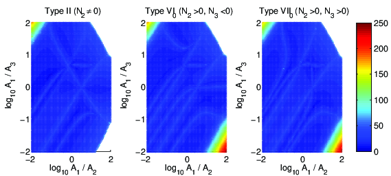
Figure 22: Here the non-zero curvature components are taken to be $\mathcal{N}_{2}>0$, $\mathcal{N}_{2}>0,\mathcal{N}_{3}<0$ and $\mathcal{N}_{2}>0,\mathcal{N}_{3}>0$ for type II, VI₀ and VII₀ respectively. Since $\mathcal{N}_{1}=0$, oscillation is allowed in top-right corner for which initially $\mathcal{A}_{1}\gg\mathcal{A}_{2},\mathcal{A}_{3}$.

Interestingly, in this scheme, the disappeared oscillation is almost completely substituted by a prolonged period of anisotropic inflation. This observation agrees with the results for type I in section 4.

References

- [1] A. Starobinsky, A new type of isotropic cosmological models without singularity, Physics Letters B 91 (Mar., 1980) 99–102.
- [2] K. Sato, First-order phase transition of a vacuum and the expansion of the Universe, Monthly Notices of the Royal Astronomical Society 195 (May, 1981) 467–479.
- [3] A. H. Guth, Inflationary universe: A possible solution to the horizon and flatness problems, Physical Review D 23 (Jan., 1981) 347–356.
- [4] A. Albrecht and P. Steinhardt, Cosmology for Grand Unified Theories with Radiatively Induced Symmetry Breaking, Physical Review Letters 48 (Apr., 1982) 1220–1223.
- [5] A. Linde, A new inflationary universe scenario: A possible solution of the horizon, flatness, homogeneity, isotropy and primordial monopole problems, Physics Letters B 108 (Feb., 1982) 389–393.
- [6] A. Linde, Chaotic inflation, Physics Letters B 129 (Sept., 1983) 177–181.
- [7] A. Linde, Particle Physics and Inflationary Cosmology, Contemporary Concepts in Physics 5 (Mar., 2005) 270, [0503203].
- [8] A. Linde, Inflation and String Cosmology, Progress of Theoretical Physics Supplement 163 (Mar., 2006) 295–322, [0503195].
- [9] A. Linde, Inflationary Cosmology, vol. 738 of Lecture Notes in Physics. Springer Berlin Heidelberg, Berlin, Heidelberg, May, 2008.
- [10] L. McAllister and E. Silverstein, String cosmology: a review, General Relativity and Gravitation 40 (Jan., 2008) 565–605, [arXiv:0710.2951].
- [11] D. H. Lyth, Inflationary Cosmology, vol. 738 of Lecture Notes in Physics. Springer Berlin Heidelberg, Berlin, Heidelberg, Feb., 2008.
- [12] P. K. Townsend, Cosmic Acceleration and M-Theory, in ICMP2003, (Lisbon), Aug., 2003. 0308149.
- [13] S. Kachru, R. Kallosh, A. Linde, and S. Trivedi, de Sitter vacua in string theory, Physical Review D 68 (Aug., 2003) 046005, [0301240].
- [14] S. Kachru, R. Kallosh, A. Linde, J. Maldacena, L. McAllister, and S. P. Trivedi, Towards inflation in string theory, Journal of Cosmology and Astroparticle Physics 2003 (Oct., 2003) 013–013, [0308055].
- [15] A. Maleknejad, M. M. Sheikh-Jabbari, and J. Soda, Gauge Fields and Inflation, Physics Reports 528 (Dec., 2013) 161–261, [arXiv:1212.2921].
- [16] S. Yokoyama and J. Soda, Primordial statistical anisotropy generated at the end of inflation, Journal of Cosmology and Astroparticle Physics 2008 (Aug., 2008) 005, [arXiv:0805.4265].
- [17] M.-a. Watanabe, S. Kanno, and J. Soda, Inflationary Universe with Anisotropic Hair, Physical Review Letters 102 (May, 2009) 191302, [arXiv:0902.2833].
- [18] N. Bartolo, E. Dimastrogiovanni, S. Matarrese, and A. Riotto, Anisotropic trispectrum of curvature perturbations induced by primordial non-Abelian vector fields, Journal of Cosmology and Astroparticle Physics 2009 (Nov., 2009) 028–028, [arXiv:0909.5621].
- [19] N. Bartolo, E. Dimastrogiovanni, S. Matarrese, and A. Riotto, Anisotropic Bispectrum of Curvature Perturbations from Primordial Non-Abelian Vector Fields, Journal of Cosmology and Astroparticle Physics 2009 (Oct., 2009) 015–015, [arXiv:0906.4944].
- [20] K. Dimopoulos, M. Karciauskas, D. H. Lyth, and Y. Rodríguez, Statistical anisotropy of the curvature perturbation from vector field perturbations, Journal of Cosmology and Astroparticle Physics 2009 (May, 2009) 013–013, [arXiv:0809.1055].
- [21] P. V. Moniz and J. Ward, Gauge field back-reaction in Born–Infeld cosmologies, Classical and Quantum Gravity 27 (Dec., 2010) 235009, [arXiv:1007.3299].
- [22] T. R. Dulaney and M. I. Gresham, Primordial power spectra from anisotropic inflation, Physical Review D 81 (May, 2010) 103532, [arXiv:1001.2301].
- [23] A. E. Gümrükçüoğlu, B. Himmetoglu, and M. Peloso, Scalar-scalar, scalar-tensor, and tensor-tensor correlators from anisotropic inflation, Physical Review D 81 (Mar., 2010) 063528, [arXiv:1001.4088].
- [24] M.-a. Watanabe, S. Kanno, and J. Soda, The Nature of Primordial Fluctuations from Anisotropic Inflation, Progress of Theoretical Physics 123 (June, 2010) 1041–1068, [arXiv:1003.0056].
- [25] R. Emami, H. Firouzjahi, S. M. S. Movahed, and M. Zarei, Anisotropic Inflation from Charged Scalar Fields, Journal of Cosmology and Astroparticle Physics 2011 (Oct., 2010) 005–005, [arXiv:1010.5495].
- [26] M.-a. Watanabe, S. Kanno, and J. Soda, Imprints of the anisotropic inflation on the cosmic microwave background, Monthly Notices of the Royal Astronomical Society: Letters 412 (Mar., 2011) L83–L87, [arXiv:1011.3604].
- [27] K. Murata and J. Soda, Anisotropic inflation with non-abelian gauge kinetic function, Journal of Cosmology and Astroparticle Physics 2011 (June, 2011) 037–037, [arXiv:1103.6164].
- [28] M. Shiraishi and S. Yokoyama, Violation of the Rotational Invariance in the CMB Bispectrum, Progress of Theoretical Physics 126 (Nov., 2011) 923–935, [arXiv:1107.0682].
- [29] R. Namba, Curvature Perturbations from a Massive Vector Curvaton, arXiv:1207.5547.
- [30] N. Bartolo, S. Matarrese, M. Peloso, and A. Ricciardone, The anisotropic power spectrum and bispectrum in the f(phi) F^2 mechanism, arXiv:1210.3257.
- [31] N. Barnaby, R. Namba, and M. Peloso, Phenomenology of a pseudo-scalar inflaton: naturally large nongaussianity, Journal of Cosmology and Astroparticle Physics 2011 (Apr., 2011) 009–009, [arXiv:1102.4333].
- [32] M. M. Anber and L. Sorbo, Non-Gaussianities and chiral gravitational waves in natural steep inflation, Physical Review D 85 (June, 2012) 123537, [arXiv:1203.5849].
- [33] S. Kanno, J. Soda, and M.-a. Watanabe, Cosmological magnetic fields from inflation and backreaction, Journal of Cosmology and Astroparticle Physics 2009 (Dec., 2009) 009–009, [arXiv:0908.3509].
- [34] N. Barnaby, R. Namba, and M. Peloso, Observable non-Gaussianity from gauge field production in slow roll inflation, and a challenging connection with magnetogenesis, Physical Review D 85 (June, 2012) 123523, [arXiv:1202.1469].
- [35] R. J. Ferreira, R. K. Jain, and M. S. Sloth, Inflationary magnetogenesis without the strong coupling problem, Journal of Cosmology and Astroparticle Physics 2013 (Oct., 2013) 004–004.
- [36] C. A. Valenzuela-Toledo, Y. Rodríguez, and D. H. Lyth, Non-Gaussianity at tree and one-loop levels from vector field perturbations, Physical Review D 80 (Nov., 2009) 103519, [arXiv:0909.4064].
- [37] C. A. Valenzuela-Toledo and Y. Rodríguez, Non-gaussianity from the trispectrum and vector field perturbations, Physics Letters B 685 (Mar., 2010) 120–127, [arXiv:0910.4208].
- [38] E. Dimastrogiovanni, N. Bartolo, S. Matarrese, and A. Riotto, Non-Gaussianity and Statistical Anisotropy from Vector Field Populated Inflationary Models, Advances in Astronomy 2010 (Jan., 2010) 1–21, [arXiv:1001.4049].
- [39] M. Karciauskas, The Primordial Curvature Perturbation from Vector Fields of General non-Abelian Groups, Journal of Cosmology and Astroparticle Physics 2012 (Apr., 2011) 014–014, [arXiv:1104.3629].
- [40] C. A. Valenzuela-Toledo, Y. Rodríguez, and J. P. B. Almeida, Feynman-like rules for calculating n -point correlators of the primordial curvature perturbation, Journal of Cosmology and Astroparticle Physics 2011 (Oct., 2011) 020–020, [arXiv:1107.3186].
- [41] R. K. Jain and M. S. Sloth, On the non-Gaussian correlation of the primordial curvature perturbation with vector fields, Journal of Cosmology and Astroparticle Physics 2013 (Feb., 2013) 003–003, [arXiv:1210.3461].
- [42] Y. Rodríguez, J. P. B. Almeida, and C. A. Valenzuela-Toledo, The different varieties of the Suyama-Yamaguchi consistency relation and its violation as a signal of statistical inhomogeneity, Journal of Cosmology and Astroparticle Physics 2013 (Apr., 2013) 039–039, [arXiv:1301.5843].
- [43] J. P. B. Almeida, Y. Rodríguez, and C. A. Valenzuela-Toledo, The Suyama-Yamaguchi consistency relation in the presence of vector fields, Modern Physics Letters A 28 (Feb., 2013) 1350012, [arXiv:1112.6149].
- [44] M. M. Anber and L. Sorbo, Naturally inflating on steep potentials through electromagnetic dissipation, Physical Review D 81 (Feb., 2010) 043534, [arXiv:0908.4089].
- [45] J. M. Wagstaff and K. Dimopoulos, Particle production of vector fields: Scale invariance is attractive, Physical Review D 83 (Jan., 2011) 023523, [arXiv:1011.2517].
- [46] K. Dimopoulos, G. Lazarides, and J. M. Wagstaff, Eliminating the -problem in SUGRA hybrid inflation with vector backreaction, Journal of Cosmology and Astroparticle Physics 2012 (Feb., 2012) 018–018, [arXiv:1111.1929].
- [47] S. Kanno, J. Soda, and M.-a. Watanabe, Anisotropic power-law inflation, Journal of Cosmology and Astroparticle Physics 2010 (Dec., 2010) 024–024, [arXiv:1010.5307].
- [48] S. r. Hervik, D. F. Mota, and M. Thorsrud, Inflation with stable anisotropic hair: is it cosmologically viable?, Journal of High Energy Physics 2011 (Nov., 2011) 146, [arXiv:1109.3456].
- [49] T. Q. Do and W. F. Kao, Anisotropic power-law inflation for the Dirac-Born-Infeld theory, Physical Review D 84 (Dec., 2011) 123009.
- [50] T. Q. Do, W. F. Kao, and I.-C. Lin, Anisotropic power-law inflation for a two scalar fields model, Physical Review D 83 (June, 2011) 123002.
- [51] J. Ohashi, J. Soda, and S. Tsujikawa, Anisotropic power-law k-inflation, arXiv:1310.3053.
- [52] K. Yamamoto, Primordial fluctuations from inflation with a triad of background gauge fields, Physical Review D 85 (June, 2012) 123504, [arXiv:1203.1071].
- [53] K.-i. Maeda and K. Yamamoto, Inflationary dynamics with a non-Abelian gauge field, Physical Review D 87 (Jan., 2013) 023528, [arXiv:1210.4054].
- [54] A. Maleknejad and M. M. Sheikh-Jabbari, Non-Abelian gauge field inflation, Physical Review D 84 (Aug., 2011) 043515, [arXiv:1102.1932].
- [55] A. Maleknejad, M. Sheikh-Jabbari, and J. Soda, Gauge-flation and cosmic no-hair conjecture, Journal of Cosmology and Astroparticle Physics 2012 (Jan., 2012) 016–016, [arXiv:1109.5573].
- [56] P. Adshead and M. Wyman, Natural Inflation on a Steep Potential with Classical Non-Abelian Gauge Fields, Physical Review Letters 108 (June, 2012) 261302, [1202.2366].
- [57] P. Adshead and M. Wyman, Gauge-flation trajectories in chromo-natural inflation, Physical Review D 86 (Aug., 2012) 043530, [arXiv:1203.2264].
- [58] M. Sheikh-Jabbari, Gauge-flation vs chromo-natural inflation, Physics Letters B 717 (Oct., 2012) 6–9, [arXiv:1203.2265].
- [59] E. Martinec, P. Adshead, and M. Wyman, Chern-Simons EM-flation, Journal of High Energy Physics 2013 (Feb., 2013) 27, [arXiv:1206.2889].
- [60] E. Dimastrogiovanni, M. Fasiello, and A. J. Tolley, Low-Energy Effective Field Theory for Chromo-Natural Inflation, arXiv:1211.1396.
- [61] P. Adshead, E. Martinec, and M. Wyman, Perturbations in Chromo-Natural Inflation, arXiv:1305.2930.
- [62] P. Adshead, E. Martinec, and M. Wyman, Gauge Fields and Inflation: Chiral Gravitational Waves, Fluctuations and the Lyth Bound, arXiv:1301.2598.
- [63] H. Funakoshi and S. Renaux-Petel, A modal approach to the numerical calculation of primordial non-Gaussianities, Journal of Cosmology and Astroparticle Physics 2013 (Feb., 2013) 002–002, [arXiv:1211.3086].
- [64] Planck Collaboration, P. A. R. Ade et al., Planck 2013 Results. XXIV. Constraints on primordial non-Gaussianity, arXiv:1303.5084.
- [65] J. Wainwright and G. F. R. Ellis, Dynamical Systems in Cosmology, vol. -1. Cambridge University Press, 1997.
- [66] R. Wald, Asymptotic behavior of homogeneous cosmological models in the presence of a positive cosmological constant, Physical Review D 28 (Oct., 1983) 2118–2120.
- [67] Y. Kitada and K.-i. Maeda, Cosmic no-hair theorem in power-law inflation, Physical Review D 45 (Feb., 1992) 1416–1419.
- [68] Y. Kitada and K.-i. Maeda, Cosmic no-hair theorem in homogeneous spacetimes, Classical and Quantum Gravity 10 (Jan., 1993) 703–734.
- [69] A. Maleknejad and M. M. Sheikh-Jabbari, Revisiting cosmic no-hair theorem for inflationary settings, Physical Review D 85 (June, 2012) 123508, [arXiv:1203.0219].
- [70] Planck Collaboration, P. A. R. Ade et al., Planck 2013 results. XXII. Constraints on inflation, arXiv:1303.5082.
- [71] G. Dvali and S.-H. Tye, Brane inflation, Physics Letters B 450 (1999), no. 1 72–82.
- [72] S. B. Giddings, S. Kachru, and J. Polchinski, Hierarchies from fluxes in string compactifications, Physical Review D 66 (Nov., 2002) 106006.
- [73] H. Ishihara, Cosmological solutions of the extended Einstein gravity with the Gauss-Bonnet term, Physics Letters B 179 (1986), no. 3 217–222.
- [74] K. Maeda, Cosmological solutions with Calabi-Yau compactification, Physics Letters B 166 (1986), no. 1 59–64.
- [75] J. Ellis, N. Kaloper, K. Olive, and J. Yokoyama, Topological R4 inflation, Physical Review D 59 (Apr., 1999) 103503.
- [76] K.-i. Maeda and N. Ohta, Inflation from M-theory with fourth-order corrections and large extra dimensions, Physics Letters B 597 (2004), no. 3 400–407.
- [77] K. Akune, K.-i. Maeda, and N. Ohta, Inflation from superstring and M-theory compactification with higher order corrections. - II. - Case of quartic Weyl terms, Physical Review D 73 (May, 2006) 103506.
- [78] K. Bamba, Z.-K. Guo, and N. Ohta, Accelerating Cosmologies in the Einstein-Gauss-Bonnet Theory with a Dilaton, Progress of Theoretical Physics 118 (Nov., 2007) 879–892.