On Convexification of Range Measurement Based Sensor and Source Localization Problems

Abstract

This manuscript is a preliminary pre-print version of a journal submission by the authors, revisiting the problem of range measurement based localization of a signal source or a sensor. The major geometric difficulty of the problem comes from the non-convex structure of optimization tasks associated with range measurements, noting that the set of source locations corresponding to a certain distance measurement by a fixed point sensor is non-convex both in two and three dimensions. Differently from various recent approaches to this localization problem, all starting with a non-convex geometric minimization problem and attempting to devise methods to compensate the non-convexity effects, we suggest a geometric strategy to compose a convex minimization problem first, that is equivalent to the initial non-convex problem, at least in noise-free measurement cases. Once the convex equivalent problem is formed, a wide variety of convex minimization algorithms can be applied. The paper also suggests a gradient based localization algorithm utilizing the introduced convex cost function for localization. Furthermore, the effects of measurement noises are briefly discussed. The design, analysis, and discussions are supported by a set of numerical simulations.

1 Introduction

Over the last decade, there has been significant amount of studies on the problem of range or distance measurement based signal source/sensor localization [1, 2, 3, 4, 5, 6, 7, 8]. This problem is formulated in abstract terms in [5] as follows:

Problem 1.1

Given known 2 or 3- dimensional sensory station positions $x_{1},\cdots,x_{N}$ ($N>2$ and $N>3$ in 2 and 3 dimensions respectively) and a signal source/target at unknown position $y^{*}$, estimate the value of $y^{*}$, from the measured distances $d_{i}=\|y^{*}-x_{i}\|$.

Problem 1.1 is defined in the form of a cooperative target/source localization task; nevertheless, it can be considered in the form of a sensor network node self-localization problem as well, where the $N$ stations represent $N$ anchors, and there is a $(N+1)$st sensor node at $y^{*}$ estimating its own position.

The major geometric difficulty of Problem 1.1 comes from the non-convex structure of optimization tasks associated with range measurements: The set of source locations corresponding to a certain distance measurement $d_{i}$ by a sensor located at point $x_{i}$ is non-convex both in two and three dimensions, in the form of a circle and a spherical shell, respectively. The generic attempt is then fusing all the distance measurements $d_{1},\dots,d_{N}$ from the sensing points $x_{1},\dots,x_{N}$, respectively, and finding the intersection of the non-convex source location sets $S(x_{i},d_{i})$ corresponding to the $(x_{i},d_{i})$ pairs. However, the non-convexity of these location sets limits the application of the algorithms devised based on intersection of the mentioned non-convex source location sets $S(x_{i},d_{i})$ and the corresponding non-convex cost functions.

This paper revisits Problem 1.1 following a different approach and suggests a geometric strategy to compose a convex geometric problem first, that is equivalent to the initially non-convex problem, at least in noise-free measurement cases. Once the convex equivalent problem is formed, a wide variety of convex minimization algorithms can be applied. The paper also suggests a gradient based localization algorithm based on the introduced convex cost function for localization. Furthermore, the effects of measurement noises are briefly discussed. The design, analysis, and discussions are supported by a set of numerical simulations.

The details of distance measurement mechanisms used for the above problem is out of scope of this paper. Such details can be found, e.g., in [7, 8]. Nevertheless, similar to [5], for better visualization of the implementation of the localization task, we give here one mechanism example, received signal strength (RSS) approach: For a source emitting a signal with source signal strength $A$ in a medium with power loss coefficient $\eta$, the RSS at a distance $d$ from the signal source is given by

$$s=A/d^{\eta}.$$ (1.1)

Using (1.1), $d$ can be calculated given values of $A$, $s$, and $\eta$.

The rest of the paper is organized as follows: Section 2 introduces the proposed problem convexification strategy based on the notion of radical axis. Section 3.1 proposes a gradient based localization algorithm minimizing the convex cost function introduced in Section 2. Convergence analysis for the noise-free measurement cases is provided in Section 3.2. Simulation studies, including those testing the effects of measurement noises, are presented in Section 4. Closing remarks are given in Section 5.

2 Convexification of the Localization Problem

2.1 Non-Convex Cost Functions

As stated in Section 1, the approaches to Problem 1.1 in the literature start with a non-convex geometric minimization problem definition and attempt to devise methods to compensate the non-convexity effects. A typical natural selection of cost function to minimize [5] is

$$J_{1}(y)=\frac{1}{2}\sum_{i=1}^{N}\lambda_{i}\left(\|x_{i}-y\|^{2}-d_{i}^{2}\right)^{2},$$ (2.1)

where $\lambda_{i}$ ($i=1,\dots,N$) are positive weighting terms. A gradient localization algorithm based on minimization of the non-convex cost function (2.1) has been proposed in [5]. Although this algorithm has proven stability and convergence properties, for these guaranteed properties to hold $y^{*}$ in Problem 1.1 is required to lie in a certain convex bounded region defined by the set $\{x_{1},\dots,x_{N}\}$. Next we introduce a new cost function to overcome the aforementioned limitation.

2.2 A Convex Cost Function Based on Radical Axes

In two dimensions, if the distance measurements $d_{i}$ in Problem 1.1 are noise-free, the global minimizer of (2.1) is located at $y^{*}$, where $J_{1}(y^{*})=0$. Geometrically, $y^{*}$ is the intersection of the circles $C(x_{i},d_{i})$ with center $x_{i}$ and radius $d_{i}$. We re-formulate this later fact to form a convex cost function to replace the non-convex (2.1), using the notion of radical axis:

Theorem 2.1

(Fact 45 of [9]) Given two non-concentric circles $C(c_{1},r_{1})$,$C(c_{2},r_{2})$, there is a unique line consisting of points $p$ holding equal powers with regard to these circles, i.e., satisfying

$${\left\|p-c_{1}\right\|}^{2}-\ {r_{1}}^{2}={\left\|p-c_{2}\right\|}^{2}-\ {r_{2}}^{2}.$$

This line is perpendicular to the line connecting $c_{1}$ and $c_{2}$, and if the two circles intersect, passes through the intersection points.

The unique line mentioned in Theorem 2.1 is called the radical axis of $C(c_{1},r_{1})$ and $C(c_{2},r_{2})$ [9].

Lemma 2.1

In 2 dimensions, if the distance measurements $d_{i}$ in Problem 1.1 are noise-free, the intersection set of the radical axes of any $N-1$ distinct circle pairs $C(x_{i},d_{i})$, $C(x_{j},d_{j})$ ($i\neq j$) is $\{y^{*}\}$.

Proof: The result straightforwardly follows from Problem 1.1 definition and the last statement of Theorem 2.1.   

In order to utilize Lemma 2.1, we first derive the mathematical representation of the radical axis $l_{ij}$ of a circle pair $C(x_{i},d_{i})$, $C(x_{j},d_{j})$ ($i\neq j$) given the values of $x_{i},x_{j},d_{i},d_{j}$. Such a radical axis line is illustrated in Figure 1.

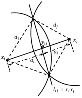
Figure 1: Radical axis of a circle pair $C(x_{i},d_{i})$, $C(x_{j},d_{j})$.

$l_{ij}$ perpendicularly intersects $x_{i}x_{j}$ at $y_{ij}$. Hence any point $y$ on it satisfies

$${(y-y_{ij})}^{T}e_{ij}=0,$$ (2.2)

where

$$e_{ij}=x_{j}-x_{i}.$$

It can be observed from Figure 1 that

$$y_{ij}=x_{i}+a_{i}\frac{e_{ij}}{\|e_{ij}\|},$$ (2.3)

as well as ${d_{i}}^{2}-{a_{i}}^{2}={d_{j}}^{2}-{a_{j}}^{2}={d_{j}}^{2}-(\|e_{ij}\|-a_{i})^{2}$, from which $a_{i}$ can be calculated as

$$a_{i}=\frac{{\|e_{ij}\|^{2}+{d_{i}}^{2}-d^{2}_{j}}}{2\|e_{ij}\|}.$$ (2.4)

The equations (2.2)–(2.4) form the explicit mathematical representation we were looking for.

Next, we focus on utilization of Lemma 2.1 to compose a convex alternative for (2.1). Leaving the optimal selection of the $N-1$ distinct circle (or corresponding sensor node) pairs to a future study, we consider a sequential pair selection for the rest of this paper: For each $i\in\{1,...,N-1\}$, let pair $i$ denote the circle pair $C(x_{i},d_{i})$, $C(x_{i+1},d_{i+1})$, $l_{i}$ denote the corresponding radical axis, $y_{i}$ denote the intersection of $l_{i}$ and $x_{i}x_{i+1}$; and according ly let us use the following special case of (2.3),(2.4):

$$y_{i} = x_{i}+a_{i}\frac{e_{i}}{\|e_{i}\|},~{}~{}e_{i}~{}=~{}x_{i+1}-x_{i},$$ (2.5)

$$a_{i} = \frac{{\|e_{i}\|^{2}+{d_{i}}^{2}-d^{2}_{i+1}}}{2\|e_{i}\|}.$$ (2.6)

Lemma 2.1 implies that the intersection set of $l_{1},\dots,l_{N-1}$ is $\{y^{*}\}$, i.e., $y^{*}$ is the unique point satisfying

$${(y-y_{i})}^{T}e_{i}=0$$ (2.7)

for all $i\in\{1,...,N-1\}$. Hence $y^{*}$ is the unique solution of the equation $J(y)=0$, where

$$J\left(y\right)=\frac{1}{2}\sum^{N-1}_{i=1}{({{\left(y-y_{i}\right)}^{T}e_{i})}^{2}}.$$ (2.8)

Observing that (2.8) is a convex cost function, we reach the following result:

Lemma 2.2

In 2 dimensions, if the distance measurements $d_{i}$ in Problem 1.1 are noise-free, then $y^{*}$ satisfies the following:

1. The radical axis lines $l_{1},\dots\l_{N-1}$ defined by (2.7) for $i=1,\dots,N-1$, respectively, intersect at $y^{*}$.

2. $y^{*}$ is the unique local minimizer and, hence, the global minimizer of (2.8).

3 Localization Algorithm

3.1 The Algorithm

As indicated above, a variety of adaptive algorithms to reach $y^{*}$ in Problem 1.1 can be devised based on the convex cost function (2.8). Here, to accommodate easy analysis and comparison with [5], we propose a gradient based adaptive algorithm, with the standard iterations of estimate updates in the negative gradient direction

$$-\nabla J(y)=-\left(\frac{\partial J(y)}{\partial y}\right)=-\sum^{N-1}_{i=1}{\left[{\left(y-y_{i}\right)}^{T}e_{i}\right]e_{i}}.$$ (3.1)

The corresponding gradient based adaptive localization algorithm is given by

$$y\left[k+1\right]=y\left[k\right]-\mu\nabla J(y[k]),$$ (3.2)

where $\mu$ is a small positive design coefficient.

3.2 Convergence Anaylsis

Because of Lemma 2.2, $\nabla J(y)=0$ if and only if $y=y^{*}$, and hence the algorithm (3.2) settles at $y[k]=y^{*}$ once it reaches that point. Further discussions on selection of the gradient gain $\mu$ and its effects on the convergence of the gradient descent algorithm (3.2) can be found in many convex optimization books, see, e.g., [10, 11, 12]. Here, we summarize the main convergence result for (3.2) with constant gain $\mu>0$:

Theorem 3.1

Consider Problem 1.1 in 2 dimensions, with noise-free distance measurements $d_{i}$. Assume that the $x_{i}$, $i\in\{1,\dots,N\}$ are non-collinear. Then for every $M>0$, there exists a $\mu^{*}(M)$ such that

$$\lim_{k\rightarrow\infty}y[k]=y^{*},$$ (3.3)

whenever

$$J(y[0])\leq M$$ (3.4)

and

$$0<\mu\leq\mu^{*}(M),$$ (3.5)

i.e., for any selection of $y[0]$, there exists a sufficiently small $\mu$ for the algorithm (3.2) such that (3.3) is satisfied.

Proof: Consider an arbitrary scalar $M>0$ and the corresponding convex st $S_{J}(M)=\{y:~{}J(y)\leq M\}$. Since (2.8) is a quadratic and hence differentiable function of $y$, it is Lipschitz within $S_{J}(M)$, i.e., there exist $L(M)$ such that for any $\bar{y}_{1},\bar{y}_{2}\in S_{J}(M)$, $\|\nabla J(\bar{y}_{1})-\nabla J(\bar{y}_{2})\|\leq L(M)$. Hence, Proposition 1.2.3 of [10] (or Theorem 1 on pp. 21 of [11]) implies that, for $y[0]\in S_{J}(M)$ and

$$0<\mu<\mu^{*}(M)=2/L(M),$$ (3.6)

we have (i) $J(y[k+1])\leq J(y[k])$, and hence $y[k]\in S_{J}(M)$ for $k=0,1,\dots$; and (ii) $\lim_{k\rightarrow\infty}\nabla J(y[k])=0$, which, by Lemma 2.1 is equivalent to (3.3).   

Remark 3.1

Theorem 3.1 implies that, in 2-D, the proposed algorithm (3.2) has global convergence property for noise-free measurement cases. Hence, using (3.2) in place of (4.1) of [5], the limitations imposed by Theorems 3.1, 3.2, 4.3 of [5] on location of $y^{*}$ will be circumvented.

4 Simulations

In this section, we present a summary of our simulations studies testing the performance of the localization algorithm proposed in the previous section. To accommodate easy and fair comparisons with the algorithm proposed in [5] and other algorithms in the literature considered in [5], we present the results for the same sample settings in that paper. For all the simulations below, the step size for algorithms (3.2) and (4.1) is selected as $\mu=0.001$, similarly to [5].

Examples 2.1 and 2.2 of [5] provide two noise free cases having false stationary points for the cost function (2.1). Example 2.1 of [5] has a single false stationary point, which is unstable. Hence, for this example, the gradient adaptive law

$$y\left[k+1\right]=y\left[k\right]-\mu\nabla J_{1}(y[k]),$$ (4.1)

using the non-convex cost function (2.1) is guaranteed to converge to the actual target position $y^{*}$ for sufficiently small $\mu$. Convergence is not guaranteed for Example 2.2 of [5], on the other hand, since there is a stable false stationary point at $[3,3]^{T}$ in this case, i.e., for a certain set of initial estimates $y[0]$, the algorithm (4.1) will converge to $[3,3]^{T}$ instead of $y^{*}=0$. It can be easily seen, based on Theorem 3.1 that this is not the case for (3.2), i.e., (3.2) converges to $y^{*}$ for both Examples 2.1 and 2.2 of [5]. The example below visualizes the second case.

Example 4.1

Consider Example 2.2 of [5], i.e. Problem 1.1 with $x_{1}=[1,1]^{T}$, $x_{2}=[1,3]^{T}$, $x_{3}=[3,1]^{T}$, and $y^{*}=0$. In this case $d_{3}^{2}=d_{2}^{2}=10$ and $d_{1}^{2}=2$. It was noted in [5] that $y^{*}_{s}=[3,3]^{T}$ is a locally stable spurious stationary point in this case for the cost function (2.1) with $\lambda_{i}=1$. A case where the estimation algorithm (4.1) produces estimates converging to $y^{*}_{s}$ instead of $y^{*}$, even with noiseless distance measurements is observed for initial estimate $y[0]=[3,2]^{2}$, as shown by the blue dashed curve in Figure 2. The black solid curve in the same figure shows the result using the proposed algorithm (3.2) for the same case and the same initial estimate,w hcih converges to the actual source position $y^{*}$.

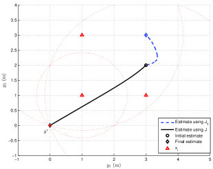
Figure 2: Example 4.1 with algorithm (4.1) of [5] (blue dashed) and the prosed algorithm (3.2) (black solid).

The next example has the same settings as the one studied in Section V of [5] with results summarized Figure 10 of that paper, with noisy RSS based measurement settings, considering continuous source emission. These settings were used in [5] to compare the performance of the gradient algorithm (4.1) with maximum likelihood estimation and Projection on Convex Sets (POCS) algorithms [3, 4]. Due to space limitations and since a comparison of (4.1) with the other aforementioned algorithms was already provided in [5], here we present only comparison of (3.2) and (4.1).

Example 4.2

Consider a network of four RSS sensors located at $[-2,-1]^{T}$, $[-1,-3]^{T}$, $[-1,1]^{T}$, $[1,0]^{T}$, subject to the signal model

$$s=\omega_{s}A/d^{\eta},$$ (4.2)

where $\omega_{s}[{\rm dB}]\triangleq 10\log\omega_{s}$ is a zero-mean Gaussian noise, i.e. $\omega_{s}[{\rm dB}]\sim\mathcal{N}(0,\sigma_{s}^{2})$. (4.2) includes a log-normal shadowing term $\omega_{s}$, as the dominant measurement noise source, in the RSS model (1.1). Let $\eta=3$. For this setting, the algorithms (3.2) and (4.1) have been comparatively tested for the shadowing noise standard deviation $\sigma_{s}$ varying from 0 to 5 dB. The mean square estimation errors for the 1000 randomly selected initial estimates and target positions (shown in Figure 3) are shown in Figures 4 and 5. Figure 4 covers the cases where the target selections are inside the ellipse, and hence convergence of (4.1) is guaranteed for $\sigma_{s}=0$, while Figure 5 covering the cases with target selections outside this ellipse. As can be seen in these figures, in addition to particular ill-conditioned cases such as the one described in Example 4.1, the proposed algorithm is effective in generic settings, especially when the shadowing noise is small.

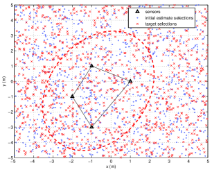
Figure 3: Random initial condition and target selections for Example 4.2. The ellipse is the one defined by Theorem 3.3. of [5]. For targets inside this ellipse, the algorithm (4.1) is guaranteed to converge with noise-free measurements.

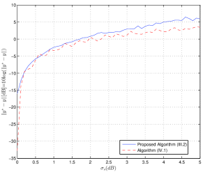
Figure 4: Average estimation error versus shadowing noise standard deviation, with targets inside the ellipsoid region guaranteing convergence of (4.1).

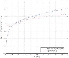
Figure 5: Average estimation error versus shadowing noise standard deviation, with targets outside the ellipsoid region guaranteing convergence of (4.1).

5 Conclusion

We have proposed a geometric strategy to define range measurement based sensor network localization of a signal source/target as a convex optimization problem. Based on this strategy we have developed a gradient based localization algorithm, which is globally convergent for noise-free measurements. In addition to formal convergence analysis, the use of the proposed strategy and algorithm is demonstrated via a set of numerical simulations. The convexity and global convergence aspects of the proposed methodology make it a good candidate for implementation, especially in precise sensor network localization tasks involving multiple targets in a wide region of interest and high precision range sensors.

References

- [1] A. Sayed, A. Tarighat, and N. Khajehnouri, “Network-based wireless location: challenges faced in developing techniques for accurate wireless location information”, IEEE Signal Processing Magazine, vol. 22, no. 4, pp. 24-40, July 2005.
- [2] N. Patwari, J. Ash, S. Kyperountas, A. Hero, R. Moses, and N. Correal, “Locating the nodes: cooperative localization in wireless sensor networks”, IEEE Signal Processing Magazine, pp. 54–69, July 2005.
- [3] A. Hero and D. Blatt, “Sensor network source localization via projection onto convex sets (POCS)”, in Proceedings of ICASSP, Vol. III, pp. III-689 – III-692, Philadelphia, P.A., March 2005.
- [4] M. Rydstrom, E. Strom, and A. Svensson, “Robust sensor network positioning based on projection onto circular and hyperbolic convex sets (POCS)”, in Proceedings of SPAWC, Cannes, France, July, 2006.
- [5] B. Fidan, S. Dasgupta, and B. Anderson, “Guaranteeing practical convergence in algorithms for sensor and source localization,” IEEE Tr. Signal Processing, vol. 56, no. 9, pp. 4458–4469, September 2008.
- [6] C. Meng, Z. Ding, and S. Dasgupta, “A semidefinite programming approach to source localization in wireless sensor networks,” IEEE Signal Processing Letters, vol. 15, pp. 253–256, 2008.
- [7] G. Mao and B. Fidan (editors), Localization Algorithms and Strategies for Wireless Sensor Networks, IGI Global, 2009.
- [8] S. Zekavat and R. Buehrer (editors), Handbook of Position Location, IEEE Press/Wiley, 2012.
- [9] R. Johnson, Advanced Euclidean Geometry, Dover Publications, 2007.
- [10] D. Bertsekas, Nonlinear Programming, Athena Scientific, 1995.
- [11] B. Polyak, Introduction to Optimization, Optimization Software, 1987.
- [12] Y. Nesterov,Introductory Lectures on Convex Optimization,Kluwer,2004.