Rotating Boson Stars in Einstein-Gauss-Bonnet gravity

Abstract

A self-interacting SU(2)-doublet of complex scalar fields, minimally coupled to Einstein-Gauss-Bonnet gravity is considered in five space-time dimensions. The classical equations admit two families of solitons corresponding to spinning and non-spinning bosons stars. The generic solutions are constructed numerically and agree with exact results that are available in special limits of the parameters. The pattern of the boson stars is shown to be qualitatively affected by the Gauss-Bonnet coupling constant.

PACS Numbers: 04.70.-s, 04.50.Gh, 11.25.Tq

1 Introduction

Boson stars and Q-balls have been known for a long time. They are non-topological solitons [1, 2] characterized by a conserved Noether charge associated with a U(1) symmetry of the Lagrangian. One of the first constructions of non-topological solitons was achieved in [3], within a field theory describing a self-interacting complex scalar field. Q-balls are classical solutions; they are stationary with an explicite time-dependent phase with frequency $\omega$. The conserved Noether charge $Q$ is then related to the global phase invariance of the theory and is directly proportional to the frequency; $Q$ can further be interpreted as the particle number. In [4], it was shown that a non-normalizable $\Phi^{6}$-potential is necessary to support soliton solutions. Using such a potential, several $Q$-ball solutions in $3+1$ dimensions have been studied in details in [4, 5, 6].

The interest for these type of classical solutions was enhanced in particular after it was shown [7, 8] that supersymmetric extensions of the Standard Model (SM) also possess $Q$-ball solutions. In [9] an effective potential involving these effects was suggested and the properties of the corresponding $Q$-balls have been investigated [10]. Many astrophysical implications have been discussed, see [11] for a non exhaustive list.

Recently several authors addressed the existence and the construction of globally regular solutions in scalar field theories coupled (minimally or not) to gravity in more than four dimensions [12],[13],[14]. Several features of the four-dimensional boson stars hold also in higher dimensions. For example the spectrum of the solutions as functions of the frequency $\omega$ present several branches existing on specific intervals of this parameter. Also, sequences of radially excited solutions exist.

Perhaps, one of the most promising way to discover new features of these solitons is to emphasize their spinning properties. Classical solutions living in d-dimensions can have $(d-1)/2$ independent angular momenta. It is therefore natural to emphasize the construction of rotating boson stars and Q-balls. The first construction of rotating boson stars in five dimensional is reported in [15]. In this paper it is shown that rotating solitons in d=5 can be accommodated if two complex scalar fields are present, assuming the two angular momenta to be equal, the classical equations leads to a system of ordinary differential equations.

With the motivation of constructing black holes with only one Killing field, the type of field configurations proposed in [15] was reconsidered in [16]. A cosmological constant was supplemented to the model and solitons as well as hairy black hole solutions have been constructed numerically. Due to the choice of a negative cosmological constant, these asymptotically ADS solutions exist without any potential for the scalar field. The extension of such objects to higher dimensions was emphasized in [19].

For $d>4$, the standard Einstein-Hilbert action is not the only possibility for modelling gravity. It is well known that a hierarchy of extended lagrangians exist while increasing the number of dimensions, say $d$. In particular for $d=5$, a Gauss-Bonnet term can be added to the Einstein-Hilbert action. It is therefore natural to study the effects of the Gauss-Bonnet term to the spectrum of boson stars. The non-spinning boson stars were constructed with Einstein-Gauss-Bonnet action in [20]. It is the purpose of this paper to extend this results for spinning solutions.

The paper is organized as follows. In section 2, we present the model, the general field equations and the ansatz allowing us to reduce these equations to a system of differential equations. Some exact results, including the asymptotic forms of the generic solutions, are presented in Sect. 3. New features of the non-spinning solutions are pointed out in section 4. The results for spinning solutions are presented in sections 5 and 6 respectively in the case of a null and negative cosmological constant. Section 7 contains conclusions.

2 The model

In this paper, we study Q-balls and boson stars for a self-interacting doublet of scalar fields in $(4+1)$-dimensional space-time and coupled to Einstein-Gauss-Bonnet gravity. The action reads :

$$S=\frac{1}{16\pi G}\int d^{5}x\sqrt{-g}\left(R-2\Lambda+\frac{\alpha}{2}\left(R^{MNKL}R_{MNKL}-4R^{MN}R_{MN}+R^{2}\right)+16\pi G{\cal L}_{\rm matter}\right)\ ,$$ (1)

where $\Lambda=-6/\ell^{2}$ is the cosmological constant, $\alpha$ the Gauss–Bonnet coupling and $M,N,K,L\in\{0,1,2,3,4\}$. The Lagrangian density for the matter fields ${\cal L}_{\rm matter}$ reads :

$${\cal L}_{\rm matter}=-\left(\partial_{M}\Phi\right)^{\dagger}\partial^{M}\Phi-U(|\Phi|)\ \ ,$$ (2)

where the scalar field $\Phi$ denotes a doublet of scalar fields : $\Phi=(\phi_{1},\phi_{2})^{t}$. Along with many authors, [9, 10], we choose the potential

$$U(|\Phi|)=m^{2}\eta_{susy}^{2}\bigg{(}1-\exp(-\frac{|\Phi|^{2}}{\eta_{susy}^{2}})\bigg{)}$$ (3)

which is constructed in such a way as to encode some relevant features of supersymmetric extensions of the standard model [9]. The parameter $m$ denotes the mass of the scalar boson while $\eta_{susy}$ is related to the energy scale below which supersymmetry is broken.

The coupled field equations for matter and gravity are obtained from the variation of the action with respect to the matter and metric fields respectively, leading to

$$\partial^{M}\partial_{M}\Phi=\frac{\partial U}{\partial\Phi}\ ,\ G_{MN}+\Lambda g_{MN}+\frac{\alpha}{2}H_{MN}=8\pi GT_{MN}\ ,$$ (4)

where $H_{MN}$ is given by

$$H_{MN}=2\left(R_{MABC}R_{N}^{ABC}-2R_{MANB}R^{AB}-2R_{MA}R^{A}_{N}+RR_{MN}\right)-\frac{1}{2}g_{MN}\left(R^{2}-4R_{AB}R^{AB}+R_{ABCD}R^{ABCD}\right)$$ (5)

and $T_{MN}$ is the energy-momentum tensor

$$T_{MN}=g_{MN}{\cal L}_{\rm matter}-2\frac{\partial{\cal L}_{\rm matter}}{\partial g^{MN}}\ .$$ (6)

Our aim is to construct gravitating, rotating solitons of the above equations. In general, such a solution would possess two independent angular momenta associated to the two orthogonal planes of rotation. Here we restrict to the case of equal angular momenta, the relevant ansatz for the metric reads [21]

$$ds^{2} = -b(r)dt^{2}+\frac{1}{f(r)}dr^{2}+g(r)d\theta^{2}+h(r)\sin^{2}\theta\left(d\varphi_{1}-W(r)dt\right)^{2}+h(r)\cos^{2}\theta\left(d\varphi_{2}-W(r)dt\right)^{2}$$ (7)

$$+ \left(g(r)-h(r)\right)\sin^{2}\theta\cos^{2}\theta(d\varphi_{1}-d\varphi_{2})^{2}\ ,$$

where $\theta$ runs from $0$ to $\pi/2$, while $\varphi_{1}$ and $\varphi_{2}$ are in the range $[0,2\pi]$. The corresponding space-times possess two rotation planes at $\theta=0$ and $\theta=\pi/2$ and the isometry group is $\mathbb{R}\times U(2)$. The metric above still leaves the diffeomorphisms related to the definitions of the radial variable $r$ unfixed; for the numerical construction, we will fix this freedom by choosing $g(r)=r^{2}$. The metric (7) then leads to a consistent system of differential equations [15] when the doublet of scalar fields is of the form

$$\Phi=\phi(r)e^{i\omega t}\hat{\Phi}$$ (8)

where $\hat{\Phi}$ is a doublet of unit length depending on the angles only. It needs to be fixed appropriately for static or rotating solutions. For static solutions, we have $\hat{\Phi}=(1,0)^{t}$ while for rotating solutions the form

$$\hat{\Phi}=(\sin\theta e^{i\varphi_{1}},\cos\theta e^{i\varphi_{2}})^{t}$$ (9)

guarantees the consistency of the ansatz. The general field-equations are transformed into a set of five differential equations for the functions $f(r),b(r),h(r),W(r)$ and $\phi(r)$

These equations depend on five independent constants: the Newton’s constant $G$, the cosmological constant $\Lambda$ (or the Anti-de Sitter radius $L$), the Gauss-Bonnet parameter $\alpha$, the mass of the scalar field $m$, and the parameter $\eta_{susy}$.

In the case $\Lambda=0$, the parameters $\eta_{susy}$ can be absorbed in a redefinition of the scale of the scalar field while the mass parameter can be absorbed in a rescaling of the space-time coordinates $x_{M}$. With these conventions and the rescaling, the fields equations depend on two dimensionless parameters : the Gauss-Bonnet parameter $\alpha$ and $\kappa\equiv 16\pi G\eta_{susy}^{2}$. In the case $\Lambda<0$, the boson stars exist even in the absence of a potential ($m=0$). An appropriate rescaling can then be used to set $\ell$ and $\kappa$ to particular values.

It might be useful to contrast the effective (or ’reduced’) matter-lagrangian densities $\sqrt{-g}{\cal L}_{matter}$ for the non-spinning and spinning cases. In the non-spinning case, the field-equations further imply $h=r^{2}$, $W(r)=0$; the effective lagrangian for the matter field simplifies to

$${\cal L}_{eff}=r^{3}\sin\theta\cos\theta\sqrt{\frac{b}{f}}\left(-U(\phi)-f(\phi^{\prime})^{2}+\omega^{2}\frac{\phi^{2}}{b}\right)$$ (10)

In the spinning case, the corresponding formula is slightly more involved :

$${\cal L}_{eff}=r^{2}\sin\theta\cos\theta\sqrt{\frac{bh}{f}}\left(-U(\phi)-f(\phi^{\prime})^{2}+\omega^{2}\frac{\phi^{2}}{b}-\phi^{2}(\frac{1}{h}+\frac{2}{g})-\frac{W^{2}}{b}-2\frac{\omega W}{b}\right)$$ (11)

The effective action densities for the Einstein-Hilbert and Gauss-Bonnet terms for the metric ansatz (7) can be found e.g. in [22].

3 Exact solutions and asymptotics

As pointed out already, the ansatz above transforms the field equations (4) into a set of five ordinary differential equations. In order to provide physically meaningful solutions, suitable conditions have to be imposed at $r=0$ (regularity at the origin) and asymptotically (localized solution in flat or AdS space-time). Only for specific limits of the coupling constants do the solutions admit a closed form. In this section we present a few exact results and the behaviour of the solution for $r\rightarrow 0$ and $r\to\infty$ in the generic case.

3.1 Asymptotics

As we want to construct solutions that are regular and localized in space and asymptotically flat, several appropriate boundary conditions should be imposed. For $r\to\infty$, the metric should approach Minkowski space-time and the matter fields should vanish. This implies the following behaviour of the five radial functions :

$$f(r)=1+\frac{{\cal U}}{r^{2}}+o(\frac{1}{r^{4}})\ \ ,\ \ b(r)=1+\frac{{\cal U}}{r^{2}}+o(\frac{1}{r^{4}})$$ (12)

$$h(r)=r^{2}(1+o(\frac{1}{r^{4}}))\ \ ,\ \ w(r)=\frac{{\cal W}}{r^{4}}\ \ ,\ \ \phi(r)\sim\frac{1}{r^{3/2}}\exp{-r\sqrt{m^{2}-\omega^{2}}}$$ (13)

The parameters ${\cal U,W}$ in the asymptotic expansion are used to determine the mass $M$ and angular momentum $J$ of the solutions :

$$M=-3\frac{V_{3}}{16\pi G}{\cal U}\ \ ,\ \ J=\frac{V_{3}}{8\pi G}{\cal W}\ \ ,\ \ V_{3}=2\pi^{2}\ .$$ (14)

3.2 Taylor expansion

In order to study the behaviour of the solutions around the origin, a Taylor expansion of the solutions can be done. We report it only in the non rotating case, (the expressions become lengthy and not illuminating in the non-rotating case). For convenience we use $A^{2}\equiv b/f$ and let

$$f(r)=1+f_{2}r^{2}+f_{4}r^{4}\ \ ,\ \ A=A_{0}+A_{2}r^{2}+A_{4}r^{4}\ \ ,\ \ \phi(r)=F_{0}+F_{2}r^{2}+F_{4}r^{4}+\dots$$ (15)

Then expanding the field equations in powers of $r$ imply that all coefficients are determined in terms of $F_{0}$ and $A_{0}$. In particular, for the quadratic terms, we find

$$f_{2}=\frac{1}{6\alpha A_{0}}\left(3A_{0}\pm\sqrt{3}\sqrt{3A_{0}^{2}+2\kappa\alpha(A_{0}^{2}U(f_{0})+\omega^{2}F_{0}^{2})}\right)$$ (16)

$$A_{2}=\frac{\kappa\omega^{2}F_{0}^{2}}{3A_{0}(1-2\alpha f_{2})}\ \ ,\ \ F_{2}=\frac{U^{\prime}(F_{0})-2F_{0}\omega^{2}}{16A_{0}^{2}}$$ (17)

The expansion suggests that two solutions should exist for generic values of $\alpha$; they are distinguished by the arbitrary sign $\pm$ occuring in $f_{2}$. Only the solution corresponding to the ’minus sign’ however possesses a regular limit for $\alpha\to 0$. Only this branch of solutions will be emphasized in the next section.

3.3 Linearized equation: $\Lambda=0$

We note that for $\kappa=0$, the Einstein-Gauss-Bonnet equations only allow regular solutions in Minkowski space-time (irrespectively of the Gauss-Bonnet coupling constant). In the limit $\kappa=0$ and assuming for the potential of a mass term only (the mass we note $m$ in this section), global analytical solutions can be found for the underlying Klein-Gordon equation. In the non spinning case, the relevant equation for the scalar field reads

$$\phi^{\prime\prime}+\frac{3}{r}\phi^{\prime}+\left(\omega^{2}-m^{2}\right)\phi=0$$ (18)

which can be solved in terms of the modified Bessel functions $I_{1}$,$K_{1}$ for $0<\omega<m$ :

$$\phi(r)=\phi_{0}\frac{1}{r}I_{1}\big{(}\sqrt{m^{2}-\omega^{2}}r\big{)}\ \ ,\ \ {\rm for}\ \ r\ll 1\ \ ;\ \ \phi(r)=\tilde{\phi}_{0}\frac{1}{r}K_{1}\big{(}\sqrt{m^{2}-\omega^{2}}r\big{)}\ \ ,\ \ {\rm for}\ \ r\gg 1$$ (19)

The function $I_{1}(r)/r$ is finite at the origin and $K_{1}$ present the desired asymptotic behaviour. In the spinning case, the equation reads

$$\phi^{\prime\prime}+\frac{3}{r}\phi^{\prime}+\left(-\frac{3}{r^{2}}+\omega^{2}-m^{2}\right)\phi=0$$ (20)

which can be solved in terms of the modified Bessel functions $I_{2}$, $K_{2}$ :

$$\phi(r)=\phi_{0}\frac{1}{r}I_{2}\big{(}\sqrt{m^{2}-\omega^{2}}r\big{)}\ \ ,\ \ {\rm for}\ \ r\ll 1\ \ ;\ \ \phi(r)=\tilde{\phi}_{0}\frac{1}{r}K_{2}\big{(}\sqrt{m^{2}-\omega^{2}}r\big{)}\ \ ,\ \ {\rm for}\ \ r\gg 1$$ (21)

which also fulfil the relevant boundary conditions. Solving the equation with the full interacting potential leads to a global solution approaching the above functions for $r\ll 1$ and $r\gg 1$ and fixes the constant $\phi_{0},\tilde{\phi}_{0}$ in function of $\omega$. Similar results are discussed in [23] for generic values of the dimension of space-time, for different potentials in one scalar field.

3.4 Probe limit: $U=0$, $\Lambda<0$

In the presence of a (negative) cosmological constant Q-balls and boson stars exist in the absence of a potential; we assume $U=0$ in this section. In the probe limit (i.e. with $\kappa=0$), the relevant solution to the Einstein-Gauss-Bonnet equations is the AdS space-time with a modified AdS radius :

$$~{}f(r)=b(r)=1+\frac{r^{2}}{\ell_{c}^{2}}\ \ ,\ \ h(r)=r^{2}\ \ ,\ \ \frac{1}{\ell_{c}^{2}}\equiv\frac{1}{\alpha}\left[1-\sqrt{1-\frac{2\alpha}{\ell^{2}}}\right]\ .$$ (22)

In particular, the Gauss-Bonnet parameter is bounded: $\alpha\leq\ell^{2}/2$. In this background, the Klein-Gordon equation leads to the differential equation

$$(r^{3}f\phi^{\prime})^{\prime}-r^{3}\left(\frac{p}{r^{2}}-\frac{\omega^{2}}{f}\right)\phi=0\ \ ,\ \ p=0:{\operatorname{non-spinning}}\ \ ,\ \ p=3:{\rm spinning}$$ (23)

which can be solved in terms of Hypergeometric functions. For non-spinning soliton, we find

$$\phi(r)=\frac{c_{0}\ell_{c}^{4}}{(r^{2}+\ell_{c}^{2})^{2}}\phantom{A}_{2}F_{1}(\frac{4-\omega\ell_{c}}{2},\frac{4+\omega\ell_{c}}{2};3,\frac{\ell_{c}^{2}}{r^{2}+\ell_{c}^{2}})$$ (24)

The corresponding Hypergeometric function $\phantom{A}{}_{2}F_{1}(a,b;c,z)$ is divergent in the limit $z\to 1$ (see [24] p. 37) for generic values of $a,b$. However it reduces to a polynom if $a$ or $b$ is a negative integer. As a consequence, the physical relevant solutions correspond to $\omega\ell_{c}=4+2k$ for any positive integer $k$. For $k=0$, the Hypergeometric function is a constant and the solution clearly obeys the boundary conditions of the ”fundamental” boson star. The higher values of $k$ lead to radial excited solutions where $\phi(r)$ present nodes at intermediate values of $r$.

In the case of spinning soliton, we have [16]

$$\phi(r)=\frac{c_{0}r\ell_{c}^{4}}{(r^{2}+\ell_{c}^{2})^{5/2}}\phantom{A}_{2}F_{1}(\frac{5-\omega\ell_{c}}{2},\frac{5+\omega\ell_{c}}{2};3,\frac{\ell_{c}^{2}}{r^{2}+\ell_{c}^{2}})$$ (25)

with the corresponding quantization condition $\omega\ell_{c}=5+2k$. In this case also, the conditions at $r=0$ and $r=\infty$ are obeyed.

No closed form solutions exist, to our knowledge, for the coupled system (i.e. for $\kappa>0$), the exact values $\omega=4$ and $\omega=5$ are recovered in the limit of vanishing scalar field; this limit is indeed equivalent to the limit $\kappa\to 0$ through an appropriate rescaling.

The metric approaches the form (22) asymptotically and the scalar field’s decay is powerlike:

$$\phi(r)_{r\to\infty}=\frac{\langle\phi\rangle}{r^{a}}\ \ ,\ \ a=2+\sqrt{4+m^{2}}$$ (26)

where a mass term of the scalar field, say $m$, has been included for completeness and the notation $\langle\phi\rangle$ is used along many papers e.g. [16].

3.5 Chern-Simons limit: $U=0$, $\alpha=\ell^{2}/2$

As pointed out above, the solutions for $\alpha>0$, $\ell^{2}<\infty$ exist only for $2\alpha/\ell^{2}<1$. The limit $\alpha=\ell^{2}/2$ is special and known as the Chern-Simons (CS) limit [17] (see also [18]). The asymptotic form of the metric in the CS limit is special. For generic values of $\alpha$, we have

$$f(r)=\frac{r^{2}}{\ell_{c}^{2}}+1+\frac{f_{2}}{r^{2}}+O(1/r^{4})\ \ ,\ \ b(r)=\frac{r^{2}}{\ell_{c}^{2}}+1+\frac{b_{2}}{r^{2}}+O(1/r^{4})\ \,\ \ h(r)=r^{2}\left(1+\frac{h_{2}}{r^{4}}\right)\ \$$ (27)

where $\ell_{c}$ is defined above. The mass is given by

$$M=\frac{V_{3}}{16\pi G}(f_{2}-4b_{2})\sqrt{1-\frac{2\alpha}{\ell^{2}}}\ .$$ (28)

which becomes undefined for $\alpha=\ell^{2}/2$. By contrast, in the Chern-Simons limit, we have [18] :

$$f(r)=2{r^{2}}+1+{\cal V}+\frac{\tilde{f}_{2}}{r^{2}}+O(1/r^{4})\ \ ,\ \ b(r)=2{r^{2}}+1+{\cal U}+\frac{\tilde{b}_{2}}{r^{2}}+O(1/r^{4})\ \,\ \ h(r)=r^{2}\left(1+\frac{\tilde{h}_{2}}{r^{2}}\right)$$ (29)

The mass of the solution is obtained in terms of ${\cal U,V}$ (see [18] for details). In the non spinning case, we have ${\cal V}={\cal U}$ and $M=\frac{V_{3}}{8\pi G}\frac{3({\cal U}^{2}-1)}{8}$; our numerical results nicely confirmed that this value is approached by (28).

4 Non-spinning Solutions

As in the previous section discussed, the system of non-linear equations does not admit in general (to our knowledge) solutions in closed form and some numerical techniques need to be employed to construct the solutions. We used the routine COLSYS [25] based on the Newton-Raphson algorithm with adaptive grid scheme.

The effect of the Gauss-Bonnet term on five dimensional (non rotating) boson stars was analyzed in [20] with a $\phi^{6}$ potential. Many features of the solutions are qualitatively similar with the potential (3). In particular, it turns out that the numerical routine used to construct the solutions becomes inefficient for the large values of $\phi(0)$ when the parameters $\kappa$, $\alpha$ are chosen in the same range of magnitude. We attempted to understand the reason of this technical difficulty by inspecting the behaviour at the origin of the metric and of the Ricci scalar $R(r)$. In complement to the figures presented in [20], we present on ${\operatorname{Fig.\ref{non_rot}}}$ the values of $R(0)=-4(3f^{\prime\prime}(0)+b^{\prime\prime}(0)/b(0))$ and the frequency $\omega$ for $\kappa=0.1$ and three values of $\alpha$ (for instance $\alpha=0.0;0.1;1.0$).

We first discuss the solutions for Einstein gravity (i.e. for $\alpha=0$). For fixed $\kappa$ and increasing $\phi(0)$ a family of solutions can be constructed with the following features :

1. The value $b(0)$ rapidly approaches zero.

2. The values $-f^{\prime\prime}(0)$ and $-R(0)$ increases significantly.

3. The frequency $\omega$ approaches a constant.

In particular the Ricci scalar is negative for the full space-time .

The strong variations of the metric fields $f(r)$, $b(r)$ around $r=0$ cause numerical instabilities. As an example, setting $\kappa=0.1$ (e.g. see ${\operatorname{Fig.\ref{non_rot}}}$) we find $b(0)\sim 10^{-3}$, $f^{\prime\prime}(0)\sim-10^{4}$, $R(0)\sim-10^{5}$, $\omega\approx 0.89$ for $\phi(0)=8$. For $\phi(0)>10$ the numerical results become unreliable. A configuration presenting an essential singularity at the origin is likely approached (roughly speaking ’exponentially’) when the central value of the scalar field increases. Our results however cannot predict whether the limiting configuration is reached for a finite or infinite value of $\phi(0)$.

However we believe that the set of solutions that we can construct with out technique catch the essential part of the whole pattern. Indeed, in the present case and as well as for the spinning solitons (discussed below), the ${\operatorname{Q-M}}$ plot of the mass of the solutions versus the particle number $Q$ reveals that the solutions assemble in two branches forming a spike at the maximal value of $Q$, say $Q=Q_{M}$ (see e.g. several Figs. in [14]). For a given value of the particle number $Q$, the solutions with the lowest mass lies on the branch directly connected to the vacuum (corresponding to the small values of $\phi(0)$); the solutions corresponding to the high values of $\phi(0)$ have a slightly higher mass and, therefore, are likely unstable.

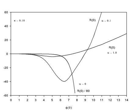
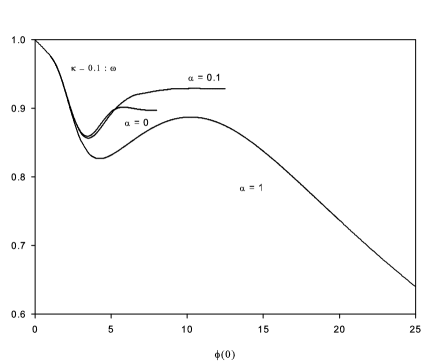
Figure 1: The Ricci scalar at the origin $R(0)$ (left) and the frequency (right) as function of $\phi(0)$ for $\kappa=0.1$ and for three values of the Gauss-Bonnet coupling $\alpha=0.0,0.1,$ and $\alpha=1.0$.

Increasing gradually the Gauss-Bonnet parameter reveals that the properties (1) and (3) above still holds. By contrast, $R(0)$ changes signs (becoming positive) and increases significantly for larger values of $\phi(0)$. This is illustrated be the $\alpha=0.1$-line in ${\operatorname{Fig.\ref{non_rot}}}$. One effect of the Gauss-Bonnet term is then a change of the sign of the curvature of space-time in the core of heavy solitons: for $r<r_{core}$, we have $R(r)\leq 0$ for $\alpha=0$, $R(r)\geq 0$ for $\alpha>0$.

Finally, for large values of $\kappa$ (typically setting $\alpha>\kappa$), the parameter $\omega$ keeps varying significantly with $\phi(0)$ (as indicated by ${\operatorname{Fig.\ref{non_rot}}}$ for the case $\alpha=1$) and the numerical integration is easier. A singular configuration seems to be approached as well, but the convergence is slower than for the small values of $\alpha$. Setting $\alpha=10$ and $\kappa=1.0$, for example, robust solutions can be constructed up to $\phi(0)\sim 50$).

The behaviour of the quantities $M,Q$ as functions of the frequency $\omega$ is largely discussed by the figures presented in [20]. It is however useful to remember some features for the next sections. The ${\operatorname{\omega-M}}$ plot reveals a series of branches assembling in the form of a spiral. For the low values of $\alpha$ (including Einstein gravity $\alpha=0$) the solitons exist for frequencies $\omega$ larger than a minimal value $\omega_{m}$ (this value off course depends on $\kappa$ and of $\alpha$). The quantities $M,Q$ are bounded.

Increasing gradually the Gauss-Bonnet parameter $\alpha$ has the effect to ’unwind’ the spiral. When $\alpha$ is chosen of the same order as $\kappa$, only one branch of solution survives extending back to the small values of $\omega$.

5 Spinning Solutions: Case $\Lambda=0$

5.1 Flat space

To calibrate the numerical results, we first studied the solitons in the case $\kappa=0$, $\alpha=0$, i.e. the rotating Q-balls interacting through the SUSY potential. The results can then be compared to the ones of [15] (our potential is bounded for $\phi\to\infty$ while the potential used in [15] grows like $\phi^{6}$). For spinning solutions, the relevant shooting parameter labeling the families of solutions is $\phi^{\prime}(0)$. As expected, our results are qualitatively similar results to [15] for the small values of $\phi^{\prime}(0)$; the corresponding scalar function is indeed small enough and confined in the region where the polynomial and SUSY potentials coincide.

On ${\operatorname{Fig.\ref{gb_0}}}$ we plot the mass, the charge (left side) and the frequency $\omega$ (right side) as functions of the parameter $\phi^{\prime}(0)$. In the limit $\phi^{\prime}(0)\to 0$ the solution corresponds to the thick wall limit and it is not well localized around the origin because $\omega\to 1$; at the same time the mass and charge increase.

The parameter $\phi^{\prime}(0)$ cannot be increased arbitrarily; indeed no solutions can be constructed for $\phi^{\prime}(0)>2.8$. At the approach of this maximal value both the mass and the charge increase considerably and likely tend to infinity. The numerical results reveal that the increase of $M$ and $Q$ is related to the fact that both the range and the amplitude of the scalar field increase although the solution is exponentially localized. When the maximal value of $\phi^{\prime}(0)$ is approached, the frequency $\omega$ reaches a plateau at $\omega\approx 0.0697$. The situation is nevertheless different from the case of non-spinning solutions (see previous section) where the mass and the charge are bounded while $\omega$ is constant.

To finish, we note that the frequency $\omega$ decreases monotonically while $\phi^{\prime}(0)$ increases; this contrasts with case of a the polynomial potential (see e.g. ${\operatorname{Fig.1}}$ of [15]). This different behavior can be explained: with a bounded potential, the ’energy cost’ for the scalar field to be large in some domain of space is smaller than for a polynomial potential.

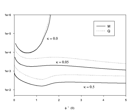
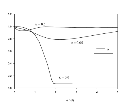
Figure 2: Mass, Charge (left) and the frequency (right) as function of $\phi^{\prime}(0)$ for three values of Newton coupling $\kappa$ and for $\alpha=0.0$.

Because the effect of the Gauss-Bonnet parameter is especially apparent when the mass and charge of the soliton are plotted in function of the frequency $\omega$, we find it useful to supplement such a plot, see ${\operatorname{Fig.\ref{gb_0_1}}}$.

Figure 3: Mass and charge of the rotating Q-balls as function of the frequency for three values of Newton coupling $\kappa$ and for $\alpha=0.0$.

5.2 Einstein gravity

Setting $\kappa>0$, the energy momentum tensor of the soliton constitutes a source term for gravity, the solutions are then boson stars. In this paper, we studied in particular the cases corresponding to $\kappa=0.05$ and $\kappa=0.5$ with the hope that it catches the main pattern. As pointed out in [15] the pattern of the gravitating solutions is qualitatively different from the ones living in flat space-time. One of the main difference (demonstrated by ${\operatorname{Fig.\ref{gb_0}}}$) is that the gravitating solutions can be constructed for larger values of the parameter $\phi^{\prime}(0)$. When the parameter $\phi^{\prime}(0)$ becomes too large, the numerical integration is problematic because the value $b(0)$ becomes very small (we could reach up to $b^{\prime}(0)\sim 0.0001$ without problem). At the same time, the value of the Ricci scalar at the origin $R(0)$ and $|f^{\prime\prime}(0)|$ increases regularly with $\phi^{\prime}(0)$ as indicated by ${\operatorname{Fig.\ref{critical_rot}}}$.

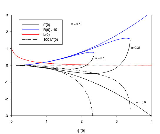
Figure 4: Several quantities characterizing the metric at the origin as function of $\phi^{\prime}(0)$ for $\kappa=0.5$ and $\alpha=0.0,0.25,$ and $\alpha=0.5$.

These numerical observations suggest that a configuration presenting a naked singularity at the origin is approached in the limit $\phi^{\prime}(0)\to\infty$. We could not find an algebraic argument demonstrating this statement.

When the mass and the charge are plotted as function of the frequency $\omega$, the graph reveals the occurence of several branches of solutions existing on different intervals of the frequency $\omega$ and forming a spiral. The first branch (say $branch_{1}$) is connected to the vacuum (i.e. $\phi(r)=0,\omega=1$) exist for $\omega_{1}\leq\omega\leq 1$. A second branch exists (say $branch_{2}$) for $\omega_{1}\leq\omega\leq\omega_{2}$ and coincides with $branch_{1}$ at $\omega=\omega_{1}$. Then a third branch exists for $\omega_{2}\leq\omega\leq\omega_{3}$. In fact several secondary branches likely exist but are not displayed on the figure. Setting, for example, $\kappa=0.05$, we find $\omega_{1}\approx 0.785$, $\omega_{2}\approx 0.98$, and $\omega_{3}\approx 0.94$. In the interval of frequencies where two or more branches coexist the solutions of $branch_{2}$ are the ones with the lowest mass; the interval $[\omega_{1},\omega_{2}]$ therefore plays a fundamental role, since it ’hosts’ the solutions with the lowest energy.

5.3 Einstein-Gauss-Bonnet gravity

We now discuss the effect of the Gauss-Bonnet term on the spinning soliton. The results reveal that, for spinning boson stars, the deformation of the Einstein soliton by the Gauss-Bonnet term obeys a different pattern with respect to the non spinning case. This effect is illustrated by ${\operatorname{Fig.\ref{mass_over_omega_005}}}$ where $\kappa=0.05$ is choosen for definiteness.

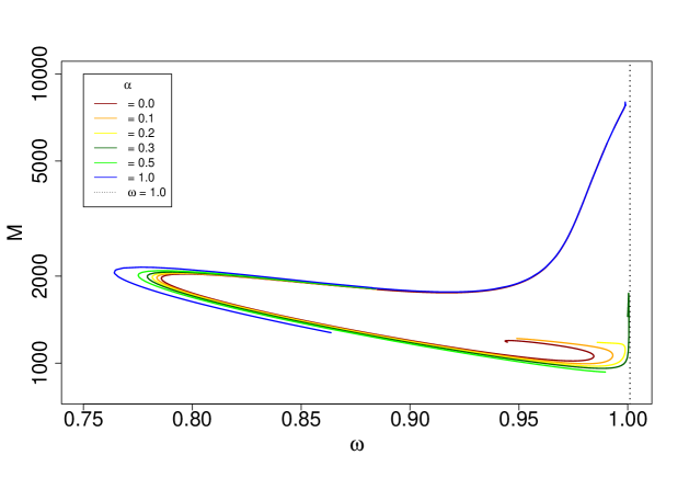
Figure 5: Mass of rotating boson stars as function of the frequency for $\kappa=0.05$ and $\alpha=0.0$ (red)$,0.1$ (orange)$,0.2$ (yellow)$,0.3$ (dark green)$,0.5$ (green), and $\alpha=1.0$ (blue).

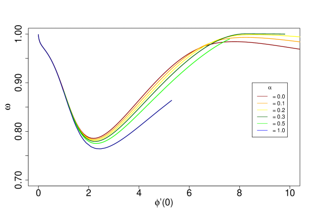
Figure 6: The frequency of rotating boson stars as function of $\phi^{\prime}(0)$ for $\kappa=0.05$ and $\alpha=0.0$ (red)$,0.1$ (orange)$,0.2$ (yellow)$,0.3$ (dark green)$,0.5$ (green), and $\alpha=1.0$ (blue).

Using the notations defined in the previous section, we focus mainly on the fundamental interval $[\omega_{1},\omega_{2}]$. It turns out that, increasing $\alpha$, the lower limit $\omega_{1}$ of the spiral decreases while the upper limit $\omega_{2}$ increases. The ’range of frequencies’ of solutions with minimal energy therefore increases with $\alpha$. In fact the upper limit of this main branch reaches and slightly overtakes the critical value $\omega=1$. This is not a contradiction with the limit $\omega=1$ (see (21)) because the corresponding solution is strongly gravitating. Such a phenomenon has, to our knowledge, not been observed so far in the study of boson stars. The numerical results show that the above pattern holds for generic values of $\kappa$. However, when $\kappa$ gets large enough (typically $\kappa=\alpha$) the spiral remains far enough from the value $\omega=1$.

As for the non-spinning case, the construction of the solutions in the large $\phi^{\prime}(0)$ limit is technically challenging. The structure of solutions reached while increasing $\phi^{\prime}(0)$ appears quite different from the $\alpha=0$ case. One aspect of this phenomenon is illustrated namely on ${\operatorname{Fig.\ref{omega_over_phidash_005}}}$ where the dependance of the frequency over the parameter $\phi^{\prime}(0)$ is presented. It shows that the curves apparently terminates at some maximal values of $\phi^{\prime}(0)$ (depending on $\alpha$) where, once more, the numerical integration becomes very problematic. A natural explanation of this phenomenon is provided by ${\operatorname{Fig.\ref{critical_rot}}}$. Here the second derivatives $f^{\prime\prime}(0),b^{\prime\prime}(0)$ and the value $R(0)$ of the Ricci scalar at the origin are reported as functions of $\phi^{\prime}(0)$ for $\kappa=0.5$ and several values of $\alpha$. It strongly suggests that when $\phi^{\prime}(0)$ approaches a ’numerical’ maximal value, the second derivatives increase significantly and even seem to become infinite for some maximal value, say $\phi^{\prime}(0)=K_{c}(\kappa,\alpha)$. At the same time the value $R(0)$ remains finite, suggesting that the limiting configuration is regular.

As a conclusion, our results indicate that (i) spinning solitons in EGB gravity exists up to a maximal value say $\phi^{\prime}(0)=K_{c}(\kappa,\alpha)$ (which depends off course on $\kappa,\alpha$); (ii) they present a maximal value of the mass, the charge and the angular momentum; (iii) the limiting configuration is regular and the divergence of $b^{\prime\prime}(0)$ and $f^{\prime\prime}(0)$ reflect an singularity due to the gauge fixing of the radial coordinate.

6 Boson stars for $\Lambda<0$, $U=0$

In the absence of a potential, one can take advantage of the rescaling of the radial variable $r$ and of the scalar field to set $\ell$ and $\kappa$ to particular values without loosing generality. Here, we have choosen $\ell=1$ and $\kappa=0.05$. The results presented in this section are obtained mainly for $U=0$; the solutions with the potential (3) will be presented in [26].

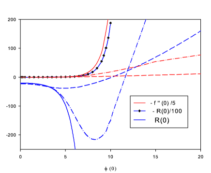
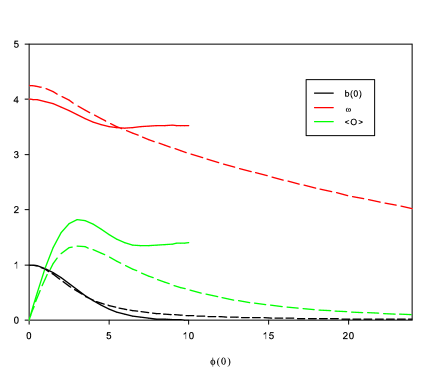
Figure 7: Left: The values $R(0)$ and $f^{\prime\prime}(0)$ versus $\phi(0)$ for $\kappa=0.05$ and $\alpha=0$ (solid lines), $\alpha=0.02$ (dot-dashed lines) and $\alpha=0.2$ (dashed lines). Right: b(0), the frequency $\omega$, and the condensate $\langle O\rangle$ as function of $\phi(0)$ for $\alpha=0$ (solid lines) and $\alpha=0.2$ (dashed lines).

We first discuss the non-spinning solutions. The pattern is similar to the case of asymptotically flat solutions.

As noticed already, the Gauss-Bonnet parameter is bounded: $0\leq\alpha\leq\ell^{2}/2$. Fixing $\alpha$ in this interval, a family of solutions can be constructed and labelled by $\phi(0)$. On ${\operatorname{Fig.\ref{ads_1}}}$, several quantities characterizing the ADS solutions for pure Einstein gravity are presented by the solid lines and the effect of the Gauss-Bonnet term appears through the dashed-dotted lines (for $\alpha=0.02$) and the dashed lines (for $\alpha=0.2$).

The general features of the system pointed out in the asymptotically flat case (see previous section) hold for AdS solutions. For $\alpha=0$, increasing the parameter $\phi(0)$ leads to configurations where the function $f(r)$ and the Ricci scalar $R(r)$ becomes very peaked at the origin. In particular the values $f^{\prime\prime}(0)$ and $R(0)$ are negative and decrease considerably as shown by ${\operatorname{Fig.\ref{ads_1}}}$. At the same time, the value $b(0)$ becomes quite small. Setting for definiteness $\kappa=0.05$, we could construct reliable solutions for $\phi(0)<10$ as reflected on both sides of ${\operatorname{Fig.\ref{ads_1}}}$: on the left side, the line with bullets demonstrate that both $R(0)$ and $f^{\prime\prime}(0)$ diverge simultaneously, on the right side the solid curves stop. Complementing ${\operatorname{Fig.\ref{ads_1}}}$, the dependance of $M$ and $Q$ on the frequency $\omega$ is shown by the solid lines of the left side of ${\operatorname{Fig.\ref{ads_2}}}$.

The requirement of the regularity conditions at the origin, together with the ADS asymptotic conditions makes it difficult to obtain reliable results for large values of $\phi(0)$ but we think however that the part of the branch that we obtained reflects the general pattern.

For $\alpha>0$, the sign of the Ricci scalar in the core of the soliton becomes positive for high enough values of $\phi(0)$, i.e. when the soliton becomes heavier. A singular-configuration seems to be approached as well but the approach is softer as demonstrated by ${\operatorname{Fig.\ref{ads_1}}}$. The mass and the charge of the CS solitons have been supplemented on ${\operatorname{Fig.\ref{ads_2}}}$ (left side) by the dashed lines. The solutions exist for $\omega\leq 4\sqrt{2}\approx 5.657$.

The main features of the solutions persist in the presence of a potential. The influence of the potential on the non-spinning solutions is sketched on ${\operatorname{Fig.\ref{ads_2}}}$ (right side) where the solid lines refer to the solution with no potential and the dashed ones to the potential (3) with $m=1$.

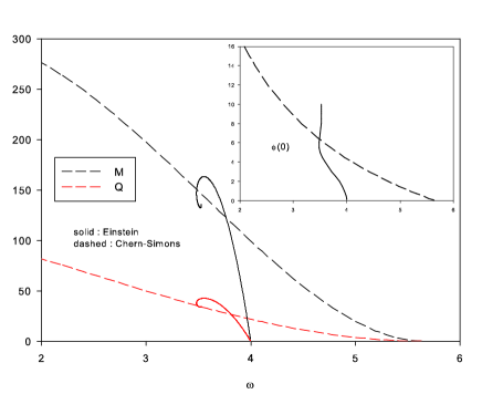
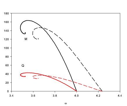
Figure 8: Left: The mass and the charge dependency on $\omega$ for the Einstein and Chern-Simons solitons (solid and dashed lines respectively). The insert contains the corresponding value $\phi(0)$. Right: The mass (black solid line) and charge (red solid line) versus $\omega$ for the family of Einstein solutions of the left side figure (i.e. with no potential) and, in the dashed lines, the same quantities for the solutions with the potential (3) with $m=1$.

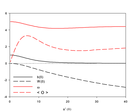
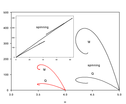
Figure 9: Left: The frequency $\omega$, the condensate $\langle O\rangle$, the value $W(0)$ and $b(0)$ as function of $\phi^{\prime}(0)$ for $\kappa=0.05$ and $\alpha=0$ for the spinning solutions with $m=0$. Right: The mass (black line) and charge (red line) versus $\omega$ for the same values for spinning and non-spinning solutions.

Finally we constructed AdS-spinning boson stars as well (for $U=0$). They present roughly the same features than their asymptotically flat counterparts and, as expected, the same numerical difficulties occur.

Several values characterizing the spinning boson stars corresponding to $\alpha=0$ are shown on ${\operatorname{Fig.\ref{ads_3}}}$, left part. The value of the rotating function at the origin $W(0)$ becomes more negative while $\phi^{\prime}(0)$ increases. The dependance of the mass and charge for the non-spinning and spinning solutions for $\alpha=0$ is presented on the right side of the figure; the two solutions exist on disjoined interval of $\omega$ terminating at the two analytical values $\omega=4$ and $\omega=5$ respectively (note: the curve for the spinning case is presented in [16] up to a rescaling of $M$ and $Q$ due to our choice $\kappa=0.05$). The ${\operatorname{Q-M}}$ plot of this data, supplemented in the insert, shows that the solutions corresponding to the large values of $\phi^{\prime}(0)$ are likely instable.

7 Conclusion

Once considered in five dimensional Minkowski or AdS space-time, the Klein Gordon equation of a doublet of massive scalar fields admits, depending on some ansatz for the angular dependency, at least two analytic solutions which are naturally localized in space. It is natural to study the deformation of these solitons when adding a suitable self-interacting potential and/or coupling the underlying scalar field to gravity. The two solutions are then promoted to stationary boson stars with or without an angular momentum. Here, we choose the Einstein-Gauss-Bonnet action for the gravitational part and a potential inspired by supersymmetric extensions of the Standard Model for the self-interacting part.

The results presented in [20] have been extended to the case of rotating boson stars. When fixing the coupling constants $\kappa,\alpha$, a family of solutions exist. It can be labeled by the value of the scalar field at the origin in the case of non-spinning solutions and by the derivative of the scalar field at the origin in the case of spinning solutions. In both cases, the construction of the solutions is technically difficult when this value becomes large enough. Our numerical results reveal new types of limiting effects which are peculiar to the Gauss-Bonnet interaction.

Once classified with respect to the frequency parameter $\omega$, multiple families of solitons (spinning or not) exist on particular intervals of $\omega$. It seems to be a generic property that, on a mass-frequency plot, these branches assemble in a spiralling shaped curve.

Increasing the value of the parameter $\phi(0)$ (for non-spinning) or of $\phi^{\prime}(0)$ (for spinning) results is a progression inside the spiral. In the case of non rotating solitons, the Gauss-Bonnet interaction has a tendency to unwind the spiral and lead, for sufficiently large values of $\alpha$ to a unique branch: one soliton for each $\omega$. For the rotating soliton the effect of the Gauss-Bonnet term is rather to enlarge the domain of $\omega$ where the first few branches of the spiral exist. The coupling to Gauss-Bonnet coupling constant leads to families of solitons existing up to a maximal value of $\phi^{\prime}(0)$, limiting the number of branches. We obtained convincing arguments that the limiting solution is regular, although some derivatives of the metric functions tend to infinity due to coordinate artefacts.

Acknowledgments We gratefully acknowledge discussions with B. Hartmann. J.R. gratefully acknowledges support within the framework of the DFG Research Training Group 1620 Models of gravity.

References

- [1] R. Friedberg, T. D. Lee and A. Sirlin, Phys. Rev. D 13 (1976) 2739.
- [2] T. D. Lee and Y. Pang, Phys. Rep. 221 (1992), 251.
- [3] S. R. Coleman, Nucl. Phys. B 262 (1985), 263.
- [4] M.S. Volkov and E. Wöhnert, Phys. Rev. D 66 (2002), 085003.
- [5] B. Kleihaus, J. Kunz and M. List, Phys. Rev. D 72 (2005), 064002.
- [6] B. Kleihaus, J. Kunz, M. List and I. Schaffer, Phys. Rev. D 77 (2008), 064025.
- [7] A. Kusenko, Phys. Lett. B 404 (1997), 285; Phys. Lett. B 405 (1997), 108.
- [8] see e.g. A. Kusenko, hep-ph/0009089.
- [9] E. Copeland and M. Tsumagari, Phys.Rev. D 80 025016 (2009).
- [10] L. Campanelli and M. Ruggieri, Phys. Rev. D 77 (2008), 043504; L. Campanelli and M. Ruggieri, Phys. Rev. D 80 (2009) 036006.
- [11] K. Enqvist and J. McDonald, Phys. Lett. B 425 (1998), 309; S. Kasuya and M. Kawasaki, Phys. Rev. D 61 (2000), 041301; A. Kusenko and P. J. Steinhardt, Phys. Rev. Lett. 87 (2001), 141301; T. Multamaki and I. Vilja, Phys. Lett. B 535 (2002), 170; M. Fujii and K. Hamaguchi, Phys. Lett. B 525 (2002), 143; M. Postma, Phys. Rev. D 65 (2002), 085035; K. Enqvist, et al., Phys. Lett. B 526 (2002), 9; M. Kawasaki, F. Takahashi and M. Yamaguchi, Phys. Rev. D 66 (2002), 043516; A. Kusenko, L. Loveridge and M. Shaposhnikov, Phys. Rev. D 72 (2005), 025015; Y. Takenaga et al. [Super-Kamiokande Collaboration], Phys. Lett. B 647 (2007), 18; S. Kasuya and F. Takahashi, JCAP 11 (2007), 019.
- [12] D. Astefanesei and E. Radu, Nucl. Phys. B 665 (2003) 594 [gr-qc/0309131].
- [13] A. Prikas, Phys. Rev. D 69 (2004) 125008 [hep-th/0404037].
- [14] B. Hartmann and J. Riedel, Phys. Rev. D 87 (2013) 4, 044003 [arXiv:1210.0096 [hep-th]].
- [15] B. Hartmann, B. Kleihaus, J. Kunz and M. List, Phys. Rev. D 82 (2010) 084022 [arXiv:1008.3137 [gr-qc]].
- [16] O. J. C. Dias, G. T. Horowitz and J. E. Santos, JHEP 1107 (2011) 115 [arXiv:1105.4167 [hep-th]].
- [17] A. H. Chamseddine, Phys. Lett. B233 (1989) 291.
- [18] Y. Brihaye and E. Radu, arXiv:1305.3531 [gr-qc], JHEP 1311 (2013) 049.
- [19] S. Stotyn, C. D. Leonard, M. Oltean, L. J. Henderson and R. B. Mann, “Numerical Boson Stars with a Single Killing Vector I: the Case,” arXiv:1307.8159 [hep-th].
- [20] B. Hartmann, J. Riedel and R. Suciu, arXiv:1308.3391 [gr-qc].
- [21] J. Kunz, F. Navarro-Lerida and A. K. Petersen, Phys. Lett. B 614 (2005) 104 [gr-qc/0503010].
- [22] Y. Brihaye and E. Radu, Phys. Lett. B 661 (2008) 167 [arXiv:0801.1021 [hep-th]].
- [23] E. J. Copeland and M. I. Tsumagari, Phys. Rev. D 80 (2009) 025016 [arXiv:0905.0125 [hep-th]].
- [24] W.Magnus, F. Oberhettinger and R. P. Soni, ”Formulas and Theorems for the Special Functions of Mathematical Physics”, Springer-Verlag, Berlin, Heidelberg, New-York (1966).
- [25] U. Ascher, J. Christiansen and R. D. Russell, Math. Comput. 33 (1979), 659; ACM Trans. Math. Softw. 7 (1981), 209.
- [26] B. Hartmann, J. Riedel and R. Suciu, Work in preparation.