A Complete Method of Comparative Statics for Optimization Problems
(Unabbreviated Version)

Abstract

A new method of deriving comparative statics information using generalized compensated derivatives is presented which yields constraint-free semidefiniteness results for any differentiable, constrained optimization problem. More generally, it applies to any differentiable system governed by an extremum principle, be it a physical system subject to the minimum action principle, the equilibrium point of a game theoretical problem expressible as an extremum, or a problem of decision theory with incomplete information treated by the maximum entropy principle. The method of generalized compensated derivatives is natural and powerful, and its underlying structure has a simple and intuitively appealing geometric interpretation. Several extensions of the main theorem such as envelope relations, symmetry properties and invariance conditions, transformations of decision variables and parameters, degrees of arbitrariness in the choice of comparative statics results, and rank relations and inequalities are developed. These extensions lend considerable power and versatility to the new method as they broaden the range of available analytical tools. Moreover, the relationship of the new method to existing formulations is established, thereby providing a unification of the main differential comparative statics methods currently in use. A second, more general theorem is also established which yields exhaustive, constraint-free comparative statics results for a general, constrained optimization problem. Because of its universal and maximal nature, this theorem subsumes all other comparative statics formulations and as such represents a significant theoretical result. The method of generalized compensated derivatives is illustrated with a variety of models, some well known, such as profit and utility maximization, where several novel extensions and results are derived, and some new, such as the principal-agent problem, the efficient portfolio problem, a model of a consumer with market power, and a cost-constrained profit maximization model, where a number of interesting new results are derived and interpreted. The large arbitrariness in the choice of generalized compensated derivatives and the associated comparative statics results is explored and contrasted to the unique eigenvalue spectrum whence all comparative statics results originate. The significance of this freedom in facilitating empirical verification and hypothesis testing is emphasized and demonstrated by means of familiar economic models. Conceptual clarity and intuitive understanding are emphasized throughout the paper, and particular attention is paid to the underlying geometry of the problems being analyzed.

I INTRODUCTION

I.1 Résumé of Current Methods

Ever since Cournot (1838) proved that a profit maximizing monopoly would reduce its output and raise its price in response to an increase in the unit tax on its output, economic theorists have sought to examine the comparative statics properties of economic theories. The epitome of such comparative statics occurred in 1886 with Antonelli and in 1915 with Slutsky, when they independently showed that the comparative statics properties of the archetype utility maximization model are summarized in a negative semidefinite matrix, now known as the Antonelli and Slutsky matrices, respectively. But it was not until the publication of Samuelson’s (1947) dissertation that comparative statics became part of the economist’s tool kit. Samuelson (1947), building upon the pioneering work of Allen (1938), Hicks (1939), and others, formulated the following strategy for deriving comparative statics results associated with optimization problems: (i) assume the second-order sufficient conditions hold at the optimal solution and apply the implicit function theorem to the first-order necessary conditions to characterize the optimal choice functions, (ii) differentiate the identity form of the first-order necessary conditions with respect to the parameter of interest, and (iii) solve the resulting linear system of comparative static equations. This primal approach is indicative of most comparative statics analyses in economics to this day, and provides the general framework within which subsequent generalizations and refinements have been carried out. Indeed, despite several extensions of Samuelson’s (1947) basic analysis by subsequent authors, the treatment of comparative statics in textbooks and monographs (with the exception of Silberberg’s [1974] contributions, discussed below), as well as in most research work, essentially relies on his original framework and for the most part ignores the subsequent developments. This circumstance is partly a result of the desire for economy of presentation. But it is undoubtedly also a consequence of the fact that none of the later extensions and generalizations of Samuelson’s (1947) basic framework succeeded in arriving at a completely general, constraint-free semidefiniteness result involving the partial derivatives of the decision variables with respect to the parameters for the case of a constrained optimization problem. In fact the existing literature does not really contemplate the general existence of such an unrestricted result [see Silberberg, (1990)].

Our objective in this paper is to show that such a general result in fact exists, that the formalism for its construction is natural and grounded in intuition, and that the comparative statics results derived from it are sufficiently broad and powerful as to render it a worthwhile tool accessible to most economists. Indeed only one extra conceptual ingredient beyond Samuelson’s (1947) basic framework is needed in its construction, namely a clear understanding of the role of compensated derivatives in formulating a general comparative statics statement. This understanding in turn leads to a recipe for identifying a suitable class of compensated derivatives in terms of which the unrestricted semidefiniteness result for a general optimization problem is realized. Before delving into details, however, it is appropriate to briefly review a few highlights of the progress since Samuelson’s (1947) seminal work, partly with a view to the concepts and methods presented in this paper. It is also appropriate at this point to recall that the standard definition of definiteness or semidefiniteness for a matrix, to which we shall adhere, requires symmetry as a prerequisite (see §IIB for a definition).

Some twenty seven years after its inception, Samuelson’s (1947) primal method was significantly advanced and enriched by a new formulation of the problem. Silberberg (1974), building upon the work of Samuelson (1965), brought about the change by means of a clever construction that in retrospect seems quite natural. By changing one’s viewpoint of the optimization problem, that is, by simultaneously considering the set of parameters and choice variables of the original, primal problem as choice variables, Silberberg (1974) set up an excess optimization problem that simultaneously contained the primal optimization problem together with a dual optimization problem, hence the appellation primal-dual. Optimization of the primal-dual problem with respect to the original choice variables yields the primal optimality conditions, while optimization with respect to the parameters yields the envelope properties of the primal optimization problem as the first-order necessary conditions, and the fundamental comparative statics properties of the primal optimization problem as the second-order necessary conditions. Undoubtedly, the most important feat achieved by the introduction of the primal-dual method was the general construction of a semidefinite matrix that contains the comparative statics properties of the primal optimization problem. The most significant shortcoming of this method, on the other hand, is the fact that its final result is subject to constraints if the optimization problem is constrained and the constraint functions depend on the parameters.

A few years later, Hatta (1980) introduced the gain method to deal with a class of optimization problems that are essentially a nonlinear, multi-constraint generalization of the Slutsky-Hicks (basic utility maximization) problem. For unconstrained problems, the gain method is identical to the primal-dual method of Silberberg (1974). For constrained problems, on the other hand, the gain method yields constraint-free comparative statics results for the above-mentioned class of problems. This is accomplished by a procedure that amounts to applying the compensation scheme used in the standard Slutsky-Hicks problem (cf. §IIC), albeit in a generalized form. Similarly, the method avoids the use of Lagrange multipliers by a comparative scheme reminiscent of Silberberg’s (1974) primal-dual method, and in effect converts the constrained problem into an unconstrained one for the gain function. This procedure is in essence equivalent to the standard multiplier method, differing only in the manner in which the auxiliary functions are introduced. Otherwise, the flavor of the analysis with the gain method is similar to that of Silberberg’s (1974) primal-dual method. Hatta’s (1980) work represents a significant advance since it succeeded in overcoming an important shortcoming in the primal-dual method by deriving the first complete, constraint-free, comparative statics results for the above-mentioned class of problems. However, it has not spurred further progress in the subject, nor has it gained wide acceptance by workers in the field, primarily because its methods are not sufficiently general and lack a clear conceptual basis.

The methods described above, and indeed most any other comparative statics analysis, rely upon the differentiability of the primitives and solution functions of the optimization problem. The recent work of Milgrom and Shannon (1994) and Milgrom and Roberts (1994), on the other hand, breaks with that tradition of dealing with the local extrema of differentiable functions. These authors, in contrast, develop an ordinal method for comparative statics, where ordinality implies invariance with respect to order-preserving transformations. Milgrom and Roberts (1994) state the following properties in defense of the ordinal method: (i) it dispenses with most of the smoothness assumptions of the traditional methods, (ii) it is capable of dealing with multiple equilibria and finite parameter changes, and (iii) it includes a theory of the robustness of conclusions with respect to assumptions. It is clear that the ordinal method is intended to handle complications which lie outside the scope of differential comparative statics methodology. As such the ordinal method is an essentially different, and in certain ways a complementary, approach to comparative statics.

Before closing this section, it is appropriate to briefly review the use of compensated derivatives in differentiable comparative statics analysis. The interest in compensated comparative statics properties of economic models has its genesis in the Slutsky matrix of compensated derivatives of the Marshallian (or ordinary) demand functions. Research on compensated comparative statics properties of general optimization problems, however, is of a more recent origin. The best known contribution of this ilk is a set of three papers by Kalman and Intriligator (1973), and Chichilnisky and Kalman (1977, 1978), which introduced generalizations that actually predated the methods described above, albeit within a restricted framework. In particular, these authors emphasized the significance of compensated derivatives in the context of a general class of constrained optimization problems and established the existence of a generalized Slutsky-Hicks matrix for such problems. However, they did not succeed in establishing the crucial semidefiniteness properties of this matrix in general. Perhaps because their analysis was primarily concerned with establishing the existence of solutions using essentially primal methods, and because their comparative statics results were restricted to special forms, their work was largely superseded by subsequent developments. Similarly, their construction and use of compensated derivatives, although a significant advance toward a general method of dealing with constraints, was rendered in the same limited context and was not much pursued by others.

The last contribution to be mentioned here is the work of Houthakker (1951-52) which, while perhaps not as well recognized as the other post-Samuelsonian contributions mentioned above, actually predates them. In an attempt to quantify the role of quality in consumer demand, Houthakker (1951-52) clearly recognized the important role played by compensated derivatives, the large number of ways in which they can be constructed, and how they are related to a differential characterization of the constraints present in the problem, albeit in the context of specific examples. However, he only succeeded in deriving the desired semidefiniteness condition for a restricted class of problems, and his contribution did not lead to any significant development in the subject.

I.2 Generalized Compensated Derivatives

As mentioned before, the method presented here is based on the pivotal role played by compensated derivatives, and in effect unifies and generalizes the above-described formulations. As is often the case, this generalization leads to a conceptually simpler structure, while yielding a powerful method of deriving constraint-free comparative statics results. The basic idea originates in the observation that the natural parameters of a given optimization problem are not necessarily the most advantageous variables for formulating comparative statics results. This is plainly obvious in the Slutsky-Hicks problem where a linear combination of derivatives in the form of a compensated derivative must be employed in order to obtain the desired semidefiniteness properties. On the other hand, a linear combination of partial derivatives is, aside from an inessential scale factor, simply a directional derivative pointed in some direction in parameter space. Since an uncompensated (i.e., a partial) derivative is also a directional derivative, albeit a very particular one pointed along one of the coordinate axes in parameter space, it follows that the distinction between the two is merely a matter of the choice of coordinates in parameter space and has no intrinsic standing. Indeed a local rotation in parameter space, i.e., a rotation whose magnitude and direction may vary from point to point, can interchange the role of the two. Such a rotation is of course equivalent to adopting a new set of parameters for the optimization problem, suitably constructed as functions of the original ones. Clearly then, any general formulation of differential comparative statics must consider the possibility of choosing from this vastly enlarged class of directional derivatives in parameter space.

The question that arises at this juncture is whether there exists a universal criterion for choosing the compensated derivatives so as to guarantee the desired semidefiniteness properties free of constraints, and without requiring any restriction on the structure of the optimization problem. Remarkably, and in retrospect not surprisingly, there is a simple and natural answer to this question. One simply chooses the compensated derivatives in conformity with the constraint conditions, i.e., along directions that are tangent to the level surfaces of all the constraint functions at each point of the parameter space (for a given value of the decision variables). Equivalently, acting on the constraint functions, the compensated derivatives are required to return zero at all points of parameter space (for a given value of the decision variables). This requirement is in effect the ab initio, differential implementation of the constraints, as will become clear in the course of the following analysis. What is perhaps more remarkable, however, is that this procedure yields an operationally powerful, yet intuitively palatable framework that is capable of yielding varied and novel results, even in the case of unconstrained problems.

Before embarking upon the following development, it is worth identifying its main elements. The cornerstone of the analysis is Lemma 1 in §IIA, the main mathematical device is the generalized compensated derivative, also developed in §IIA, and the principal result of the analysis is Theorem 1 in §IIB. This is followed by several auxiliary developments and extensions, most of which are summarized in Theorem 2 and the Corollaries in §IIB and IIC. In §IID we establish a maximal extension of Theorem 1, a theoretically important result which implies all other comparative statics formulations. The method of generalized compensated derivatives is applied in §III to a number of models, some old and several new, where its power and flavor are illustrated.

II DEVELOPMENT OF THE MAIN RESULTS

This section is devoted to a detailed development of the main tools and results of the present method according to the ideas described above. Because the underlying structure of this method is simple and natural, we find it worthwhile to continue emphasizing the intuitive aspects of the analysis in the following development. It is our hope that a clear conceptual grasp of its basics will encourage its use among a wider segment of economists.

II.1 Geometry of Generalized Compensation

To convey a clear picture of how the ideas described in §IB are implemented, we find it helpful to describe the geometrical background involved in the construction of compensated derivatives in some detail. Let us first recall certain basic results from analysis. Consider a real-valued, continuously differentiable function $\phi(\mathbf{x},\mathbf{a})$ defined for $\bf a$ in some open subset ${\cal P}$ of ${\Re}^{N}$ and $\bf x$ in a subset ${\cal D}$ of ${\Re}^{M}$. This function will later be identified with an objective or constraint function, with the $M$-dimensional vector $\mathbf{x}=(x_{1},x_{2},\ldots,x_{M})$ representing the decision variables in the decision space, and the $N$-dimensional vector $\mathbf{a}=(a_{1},a_{2},\ldots,a_{N})$ representing a set of $N$ parameters in the parameter space . For most of this section, the dependence of $\phi$ on $\bf x$ plays a secondary role in the discussion, so that it is useful to consider $\bf x$ as fixed and $\phi$ as a continuously differentiable function defined on an open subset $\cal P$ of $\Re^{N}$. Throughout the paper, we will symbolize vectors and matrices both in “vector” and “matrix” notation, as in $\bf v$ and $\sf{M}$, and in “component” notation, as in ${v}_{i}$ and ${\sf{M}}_{ij}$. The inner product of two vectors $\bf v$ and $\bf u$ is denoted by $\mathbf{v}\cdot\mathbf{u}\stackrel{{\scriptstyle\rm{def}}}{{=}}{\sum}_{i=1}^{M}{v}_{i}{u}_{i}$. For a pair of matrices $\sf{M}$ and $\sf{N}$, the product is denoted by ${\sf{M}}{\sf{N}}\stackrel{{\scriptstyle\rm{def}}}{{=}}{\sum}_{j=1}^{M}{\sf{M}}_{ij}{\sf{N}}_{jk}$. As for inner products between vectors and matrices, ${\sf{M}}\mathbf{v}$ stands for the vector (column matrix) ${\sum}_{j=1}^{M}{\sf{M}}_{ij}{v}_{j}$, $\mathbf{v}^{{\dagger}}{\sf{M}}$ stands for the vector (row matrix) ${\sum}_{j=1}^{M}{v}_{j}{\sf{M}}_{ji}$, so that $\mathbf{v}^{{\dagger}}{\sf{M}}\mathbf{u}$ stands for the scalar ${\sum}_{i,j=1}^{M}{v}_{i}{\sf{M}}_{ij}{u}_{j}$.

Given a fixed value of $\mathbf{x}$, let $\bar{\mathbf{a}}$ be a point in $\cal P$ and ${\cal S}(\bar{\mathbf{{a}}})$ the $(N-1)$-dimensional level surface of $\phi$ passing through $\bar{\mathbf{{a}}}$, that is, the set of points in $\cal P$ at which $\phi$ assumes the fixed value $\phi(\mathbf{x},\bar{\mathbf{{a}}})$. In symbols, ${\cal S}(\bar{\mathbf{{a}}})\stackrel{{\scriptstyle\rm{{def}}}}{{=}}\{\mathbf{a}\in{\cal P}:\phi(\mathbf{x},\mathbf{a})=\phi(\mathbf{x},\bar{\mathbf{{a}}})\}$. Then the gradient of $\phi$ with respect to $\mathbf{a}$ at point $\bar{\mathbf{a}}$, denoted by $\mathbf{\nabla}^{\mathbf{a}}\phi(\mathbf{x},\bar{\mathbf{a}})$, is a vector normal to ${\cal S}(\bar{\mathbf{a}})$ at $\bar{\mathbf{a}}$, and represents the direction of most rapid change for $\phi$ at that point. We shall denote this vector by $\mathbf{n}(\bar{\mathbf{a}})\stackrel{{\scriptstyle\rm{{def}}}}{{=}}\mathbf{\nabla}^{\mathbf{a}}\phi(\mathbf{x},\bar{\mathbf{a}})$ and its normalized version by $\hat{\mathbf{n}}(\bar{\mathbf{a}})\stackrel{{\scriptstyle\rm{{def}}}}{{=}}{\mathbf{n}}(\bar{\mathbf{a}})/\|{\mathbf{n}}(\bar{\mathbf{a}})\|$, where $\|\mathbf{z}\|$ denotes the length of the vector $\bf z$. On the other hand, the hyperplane tangent to the level surface at $\bar{\mathbf{a}}$, denoted by ${\cal I}(\bar{\mathbf{a}})$, is generated by the set of vectors that are tangent to ${\cal S}(\bar{\mathbf{a}})$ at point $\bar{\mathbf{a}}$, and represents the directions of no change for $\phi$ at $\bar{\mathbf{a}}$. Note that ${\mathbf{n}}(\bar{\mathbf{a}})$ is orthogonal to ${\cal I}(\bar{\mathbf{a}})$. In plain language, then, the normal vector ${\mathbf{n}}(\bar{\mathbf{a}})$ represents the direction of maximum change, whereas the tangent hyperplane represents the directions of zero change, or the null directions. We shall refer to a vector in the tangent hyperplane as an isovector. Thus an isovector is any vector that points in a null direction. Together, the isovectors and the normal vector span all possible directions, thus providing a convenient local vector space at point $\bar{\mathbf{a}}$ of the parameter space. Figure 1 is an illustration of the structure just described in a three-dimensional parameter space, with $\mathbf{t}^{1}$ and $\mathbf{t}^{2}$ depicting two isovectors in the tangent hyperplane ${\cal I}(\bar{\mathbf{a}})$.

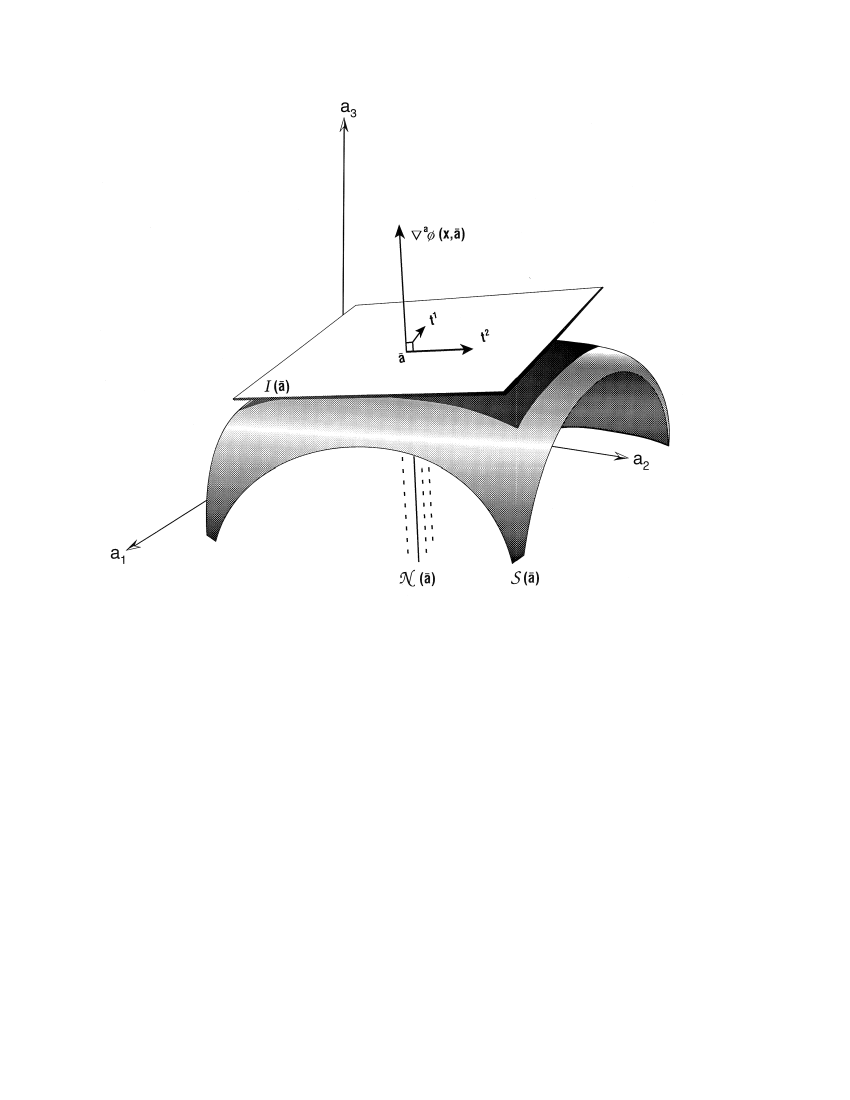
Figure 1: An illustration of the tangent plane and normal direction in a 3-dimensional parameter space. Isovectors $\mathbf{t}^{1}$ and $\mathbf{t}^{2}$ are a pair of independent vectors on the tangent plane.

To define the geometric structure described above more generally, we first consider the vector space ${\cal N}(\bar{\mathbf{{a}}})$ generated by the normal vector ${\mathbf{n}}(\bar{\mathbf{{a}}})$. While ${\cal N}(\bar{\mathbf{{a}}})$ is a one-dimensional space in the present case, it will be generalized to higher dimensions in more general situations later, and can therefore be referred to as the normal hyperplane in general. Thus we have associated with each point $\bar{\mathbf{{a}}}$ of the parameter space a pair of orthogonal vector spaces ${\cal N}(\bar{\mathbf{{a}}})$ and ${\cal I}(\bar{\mathbf{{a}}})$, the direct sum of which is the $N$-dimensional local vector space referred to above. We will denote the latter by ${\cal T}^{N}(\bar{\mathbf{{a}}})$, and refer to it as the tangent space associated with point $\bar{\mathbf{{a}}}$. This construction implies, among other things, that any real, $N$-dimensional vector can be uniquely resolved into a pair of components, one lying in the normal hyperplane and the other in the tangent hyperplane.

If we now consider all points of $\cal P$ as endowed with the tangent space structure just described, there emerges a configuration of local vector spaces covering all of $\cal P$. In terms of these local spaces, the differential structure of $\phi$ is essentially reduced to that of a function of one variable, namely the coordinate measured along the normal direction, since at a given point $\mathbf{a}\in{\cal P}$, the derivative of $\phi$ along any direction lying in the tangent hyperplane vanishes. We may summarize these results by saying that at every point $\mathbf{a}\in{\cal P}$, and for any direction specified by the (real, $N$-dimensional) unit vector $\hat{\mathbf{u}}$, (i) the decomposition $\hat{\mathbf{u}}=[\hat{\mathbf{u}}\cdot\hat{\mathbf{n}}(\mathbf{a})]\hat{\mathbf{n}}(\mathbf{a})+\mathbf{u}^{t}$, where ${\bf{u}}^{t}$ represents the projection of $\hat{\mathbf{u}}$ onto the tangent hyperplane ${\cal I}(\mathbf{a})$, is unique, and (ii) the directional derivative of $\phi$ at point $\mathbf{a}$ in the direction $\hat{\mathbf{u}}$ is given by $D^{\hat{\mathbf{u}}}\phi(\mathbf{x},\mathbf{a})\stackrel{{\scriptstyle\rm{{def}}}}{{=}}\hat{\mathbf{u}}\cdot\mathbf{\nabla}^{\mathbf{a}}\phi(\mathbf{x},\mathbf{a})=\hat{\mathbf{u}}\cdot{\mathbf{n}}(\mathbf{a})$. The last property implies that if $\hat{\mathbf{u}}$ points in a null direction, i.e., if $\hat{\mathbf{u}}\in{\cal I}(\mathbf{a})$, then the corresponding derivative vanishes: $D^{\hat{\mathbf{u}}}\phi(\mathbf{x},\mathbf{a})=0$. We shall refer to this condition as the null property of a directional derivative. Note that we have suppressed the dependence on $\mathbf{{a}}$ in $D^{\mathbf{u}}$ to avoid cluttered notation. Note also that the length of $\hat{\mathbf{u}}$ plays no role with respect to the null property, only the fact that it points in a null direction, or, equivalently, that it is an isovector. Thus if $\bf t$ is an isovector of any length, then $\mathbf{t}\cdot\mathbf{\nabla}^{\mathbf{a}}\phi(\mathbf{x},\mathbf{a})=0$, so that $\mathbf{t}\cdot\mathbf{\nabla}^{\mathbf{a}}$ possesses the null property as well. Observe that $\mathbf{t}\cdot\mathbf{\nabla}^{\mathbf{a}}$ is a linear combination of partial derivatives, equal to $\|\mathbf{t}\|D^{\hat{\mathbf{t}}}$. Since our primary focus is on the null property of this linear combination, we shall continue to (loosely) refer to $\mathbf{t}\cdot\mathbf{\nabla}^{\mathbf{a}}$ as a directional derivative, overlooking the inessential scalar factor $\|\mathbf{t}\|$ in doing so. We have thus arrived at the rather obvious conclusion that any directional derivative of a function in the direction of one of its isovectors has the null property with respect to that function.

This last property is the basis of our definition of compensated derivatives: Any linear combination of partial derivatives possessing the null property with respect to a function $\phi$ is a generalized compensated derivative (hereafter abbreviated as GCD) with respect to that function. To avoid trivialities, we shall exclude identically vanishing linear combinations from this definition. Thus any directional derivative in a null direction is a GCD, with the converse also holding except where $\mathbf{\nabla}^{\mathbf{a}}\phi(\mathbf{x},\mathbf{a})$ vanishes. As an example, consider the case illustrated in Fig. 1 where $\mathbf{t}^{1}$ and $\mathbf{t}^{2}$ depict a pair of isovectors at point $\bar{\mathbf{a}}$, which is located on the level surface ${\cal S}(\bar{\mathbf{a}})$ of $\phi(\mathbf{x},{\mathbf{a}})$. For this case, then, the directional derivatives $\mathbf{t}^{1}\cdot\mathbf{\nabla}^{\mathbf{a}}$ and $\mathbf{t}^{2}\cdot\mathbf{\nabla}^{\mathbf{a}}$ are a pair of GCD’s with respect to $\phi(\mathbf{x},{\mathbf{a}})$. Their null property, on the other hand, is seen in Fig. 1to reflect the simple fact that the rate of change of a function is zero in directions tangent to its level surface. Moreover, the reason for making the null property a defining characteristic is the crucial fact that, when the GCD’s possess this property with respect to the constraint functions, the resulting semidefiniteness results emerge free of constraints. This basic result will be established in this and the following sections.

Although our construction has so far been limited to a one-dimensional normal hyperplane, we shall consider higher-dimensional normal hyperplanes in dealing with illustrative problems, where expressions involving the normal vectors $\mathbf{\nabla}^{\mathbf{a}}\phi(\mathbf{x},\mathbf{a})$ and $\hat{\mathbf{n}}$ will be generalized to include a set of such vectors. Otherwise, the geometrical features discussed above, including the decomposition into normal and tangent components, remain unchanged.

Let us illustrate the construction of GCD’s by means of four basic economic problems. All but the third assume perfect information and are thus deterministic, while the third problem involves uncertainty as well as asymmetry of information between the transacting parties. In the first problem, the function $\phi$ is given by $\phi(\mathbf{x},\mathbf{a})\stackrel{{\scriptstyle\rm{{def}}}}{{=}}m-\mathbf{p\cdot x}$, where $\bf p$, $\mathbf{x}\in\Re_{+}^{N-1}$, and $\mathbf{x}$ is a fixed vector here. This is of course the generic form of the budget constraint that appears in the prototype utility maximization problem. Here the variables of interest are the $N$ parameters appearing in $\phi$, identified according to $\mathbf{a}=(a_{1},\ldots,a_{N})\stackrel{{\scriptstyle\rm{{def}}}}{{=}}(p_{1},\ldots,p_{N-1},m)=(\mathbf{p},m)$. Then the normal direction is given by ${\mathbf{\nabla}^{\mathbf{a}}}\phi(\mathbf{x},\mathbf{a})=(-\mathbf{x},1)$. Next, we must choose a set of $N-1$ vectors, all orthogonal to the normal direction just calculated, as a basis for the tangent hyperplane. A convenient choice is the set $\mathbf{t}^{\alpha}\stackrel{{\scriptstyle\rm{{def}}}}{{=}}(0,\ldots,1,\ldots,0,x_{\alpha})$, $\alpha=1,\ldots,N-1$, where the component equal to unity occupies the $\alpha$th position within the parenthesis. Note that these basis vectors are neither mutually orthogonal nor of unit length, but that they are all orthogonal to the gradient vector and constitute an independent set in the tangent hyperplane. Clearly, each $\mathbf{t}^{\alpha}$ is an isovector, so that the set of directional derivatives formed by taking the inner product $\mathbf{t}^{\alpha}\cdot{\mathbf{\nabla}^{\mathbf{a}}}\stackrel{{\scriptstyle\rm{{def}}}}{{=}}D_{\alpha}(\mathbf{x},\mathbf{a})$ possesses the desired null property with respect to $\phi$ and is therefore a set of $N-1$ GCD’s. Note that we have made the dependence of the GCD’s on the points $\bf x$ of the decision space and $\bf a$ of parameter space explicit in our notation, a practice which we shall henceforth follow. Remembering that here ${\mathbf{\nabla}^{\mathbf{a}}}=({\partial\over\partial{p}_{1}},\ldots,{\partial\over\partial{p}_{N-1}},{\partial\over\partial m})$, one can easily derive the result $D_{\alpha}(\mathbf{x},\mathbf{a})={\partial\over\partial{p}_{\alpha}}+{x}_{\alpha}{\partial\over\partial m}$. The latter is of course the compensated derivative that appears in the Slutsky-Hicks problem. It is worth noting here that (for $N\geq 3$) any linear combination of $D_{\alpha}(\mathbf{x},\mathbf{a})$ will again yield a GCD. This fact corresponds to the infinite number of ways one can choose $N-1$ independent basis vectors in ${\cal I}(\bf{a})$ when $N\geq 3$, and already gives a hint of the generality of the present method, and as well of the diversity of the results it can generate. It is also worth noting here that the procedure described above and applied to this problem is not the only available method for constructing GCD’s, but one that reveals the underlying geometry most explicitly. Thus any procedure that yields a set of directional derivatives with the null property and such that the corresponding directions in the parameter space span the tangent hyperplane will suffice. Taking advantage of this freedom, we will in the following sections introduce simplified procedures for constructing the set of GCD’s for various applications.

While the above treatment illustrates the construction of a GCD for a constrained problem in the context of a well known model, our second problem will deal with an unconstrained model and will give an indication of the calculational novelty of the present method.

Consider ${\tilde{\phi}}(\mathbf{x},\mathbf{a})\stackrel{{\scriptstyle\rm{{def}}}}{{=}}s[pF(\mathbf{x})-\mathbf{x}\cdot\mathbf{w}]$, where $\mathbf{x,w}\in{\Re}_{+}^{M}$. This $\tilde{\phi}$ is, except for the presence of the scale factor $s>0$, the familiar function that describes the profit of a firm producing a single output from $M$ inputs under conditions of certainty and perfect competition; here $\bf x$ is the vector of inputs, $F$ is a twice continuously differentiable production function, $p$ is the output price, and $\bf w$ is the vector of input prices. Clearly, since the scale factor $s$ is stipulated to be positive, its magnitude does not affect the optimal values of the decision variables under profit maximization, nor does it have any effect on the comparative statics of the problem. In any case, $s$ will be treated as a parameter whose value will eventually be set equal to unity. It should be evident here that the scale factor serves an auxiliary purpose in this calculation and has no other purpose, even though there are economically meaningful interpretations of its role as will be discussed in §IIB.

Let the parameter set be identified as $\mathbf{a}=(a_{1},\ldots,a_{M+2})\stackrel{{\scriptstyle\rm{{def}}}}{{=}}(w_{1},w_{2},\ldots,w_{M},p,s)=(\mathbf{w},p,s)$. Then $\mathbf{\nabla}^{\mathbf{a}}=({\partial\over\partial w_{1}},\ldots,{\partial\over\partial w_{M}},{\partial\over\partial p},{\partial\over\partial s})$, so that we find ${\mathbf{\nabla}^{\mathbf{a}}}{\tilde{\phi}}(\mathbf{x},\mathbf{a})=(-s\mathbf{x},sF,\phi)$, where $\phi(\mathbf{x},\mathbf{a})\stackrel{{\scriptstyle\rm{{def}}}}{{=}}pF(\bf x)-\mathbf{x}\cdot\mathbf{w}$ is the standard function describing the firm’s profit. Note that there are now $M+2$ parameters under consideration, so that $N=M+2$. We can therefore choose the $M+1$ isovectors according to $\mathbf{t}^{\alpha}\stackrel{{\scriptstyle\rm{{def}}}}{{=}}(0,0,\ldots,1,\ldots,0,0,{s{x}_{\alpha}\over\phi})$, $\alpha=1,2,\ldots,M$, where the component equal to unity occupies the $\alpha$th position within the parenthesis, and $\mathbf{t}^{M+1}\stackrel{{\scriptstyle\rm{{def}}}}{{=}}(0,\ldots,0,1,-s{F\over\phi})$. The corresponding set of compensated derivatives is easily found to be $D_{\alpha}(\mathbf{x},\mathbf{a})={\partial\over\partial w_{\alpha}}+({s{x}_{\alpha}\over\phi}){\partial\over\partial s}$, $\alpha=1,2,\ldots,M$, and $D_{M+1}(\mathbf{x},\mathbf{a})={\partial\over\partial p}-s{F\over\phi}{\partial\over\partial s}$. Note that each $D_{\alpha}(\mathbf{x},\mathbf{a})$ has the null property with respect to $\tilde{\phi}$. Therefore these $M+1$ directional derivatives constitute a set of GCD’s for this problem and will be used in §IIIA to derive certain novel comparative statics results for the standard profit maximization model.

It is appropriate at this juncture to emphasize an important feature of GCD’s briefly mentioned earlier. While the customary meaning of compensation refers to a correction term that accounts for the effect of a constraint in the problem, the archetypical example being the correction for the income effect in the utility maximization problem, no necessary connection with constraints is implied in the case of generalized compensation, as is clearly illustrated in the profit maximization case treated above. Indeed any problem, constrained or not, will admit the use of generalized compensation if its parameter space is larger than one-dimensional. Furthermore, as the introduction of the scale parameter $s$ for the problem treated above shows, the parameter space can always be enlarged, so that the restriction to more than one dimension is really no restriction at all.

The next problem to be considered here involves multiple constraints. It is therefore appropriate to first generalize the notion of GCD’s to the case of a set of functions $\phi^{k}(\mathbf{x},\mathbf{a})$, $k=1,2,\ldots,K$, $K<N$, each of which possesses the properties ascribed to $\phi(\mathbf{x},\mathbf{a})$ in §IIA. To that end, consider a fixed value of $\bf x$, and let $\bf a$ be a point in $\cal P$. Then the normal hyperplane ${\cal N}(\mathbf{a})$ is defined to be the vector space generated by the set of vectors ${\mathbf{n}}^{k}(\mathbf{a})\stackrel{{\scriptstyle\rm{{def}}}}{{=}}\mathbf{\nabla}^{\mathbf{a}}\phi^{k}(\mathbf{x},\mathbf{a})$, $k=1,2,\ldots,K$. Note that in case the normal vectors constitute an independent set, i.e., if the only solution to $\sum_{k=1}^{K}c^{k}{\mathbf{n}}^{k}(\mathbf{a})=0$, where every $c^{k}$ is a real number, is $c^{k}=0$ for all $k$, then the normal hyperplane will be $K$-dimensional. The subset of the tangent space ${\cal T}^{N}(\mathbf{a})$ orthogonal to ${\cal N}(\mathbf{a})$ is then the tangent hyperplane ${\cal I}(\mathbf{a})$ as before. Note that when ${\cal N}(\mathbf{a})$ has dimension $K$, i.e., when $\dim[{\cal N}(\mathbf{a})]=K$, then $\dim[{\cal I}(\mathbf{a})]=N-K$. The case of interest for economic problems usually corresponds to the condition $\dim[{\cal N}(\mathbf{a})]=K$ (known in decision space as a constraint qualification condition) with $K<N$. In any case, it should be emphasized here that what is needed for the construction of GCD’s is an independent set of isovectors which can be characterized as a set of $N-\dim[{\cal N}(\mathbf{a})]$ independent, $N$-dimensional vectors each of which is orthogonal to ${\mathbf{n}}^{k}(\mathbf{a})$ for every value of $k$. Clearly, there is no need for an explicit construction of ${\cal N}(\mathbf{a})$ here.

Having established the generalization to the multiconstraint case, we now turn to the third problem illustrating the construction of GCD’s. This is the principal-agent problem with hidden actions (also known as moral hazard) where a firm, the principal, intends to hire an individual, the agent, to work on a certain venture on a contractual basis (see, e.g., Mas-Collel et al. 1995). We shall return to this problem in §IIIB, where we define and formulate the problem, then show that it can be transformed to the following convenient form:

$${\min\;}_{\mathbf{x}}{\;}{\sum}_{i=1}^{M}{x}_{i}{\cal P}_{i}^{I}\;\;s.t.{\>}{\>}{B}^{k}-{\sum}_{i=1}^{M}v({x}_{i}){\cal P}_{i}^{k}=0,\;\;{s}^{k}-{\sum}_{i=1}^{M}{\cal P}_{i}^{k}=0,\;k=I,II,$$

Here ${\cal P}_{i}^{k}$, where $0<{\cal P}_{i}^{k}<1$, $i=1,\ldots,M$, $k=I,II$, is the probability that the $i$th profit level, ${\pi}_{i}$, is realized for the firm given that the agent performs at effort level $k$, with $I$ and $II$ corresponding to high and low effort respectively. The decision variable ${x}_{i}$, on the other hand, is the agent’s compensation in case the $i$th profit level is realized. Furthermore, ${B}^{k}\stackrel{{\scriptstyle\rm{{def}}}}{{=}}{c}^{k}+\bar{u}$, where ${c}^{k}$ is the agent’s disutility of working at effort level $k$, $\bar{u}$ is the market price of the agent’s services, and $v(x)-{c}^{k}$ is the agent’s utility function. Finally, the parameters ${s}^{k}$ are a pair of positive auxiliary variables which are introduced for calculational convenience and will eventually be set equal to unity. The parameter set is thus identified as $({\cal P}_{i}^{k},{B}^{k},{s}^{k})$, with $i=1,2,\ldots,M$ and $k=I,II$, for a total of $2(M+2)$, to be eventually reduced to $2(M+1)$ upon setting ${s}^{k}=1$.

Rather than following the procedure used in the other illustrative problems of this section, here we shall develop an intuitive generalization of the GCD’s already constructed for the Slutsky-Hicks problem. We accomplish this in two steps. In the first step, we note that for each value of $k$, the constraint ${B}^{k}-{\sum}_{i=1}^{M}v({x}_{i}){\cal P}_{i}^{k}=0$ is analogous to a budget constraint with ${B}^{k}$ standing for income, $v({x}_{i})$ for the quantity of the $i$th good, and the probability ${\cal P}_{i}^{k}$ for the price of that good. This analogy immediately gives us the two-term structure $\partial/\partial{\cal P}_{i}^{k}+v({x}_{i})\partial/\partial{B}^{k}$, $k=I,II$ which is clearly compensated (i.e., possess the null property) with respect to the constraints involving ${B}^{k}$. The second step is to amend this structure so as to extend the null property to the constraints involving ${s}^{k}$. One can determine by analogy and verify by inspection that the addition of $\partial/\partial{s}^{k}$ to the above structure provides the desired extension of the null property to the constraints involving ${s}^{k}$ without disturbing the same property with respect to the constraints involving ${B}^{k}$. In short, the resulting structure, ${d}_{i}^{k}\stackrel{{\scriptstyle\rm{{def}}}}{{=}}\partial/\partial{\cal P}_{i}^{k}+v({x}_{i})\partial/\partial{B}^{k}+\partial/\partial{s}^{k}$, has the required null property with respect to all constraints. We can thus define

$$D_{\alpha}(\mathbf{x},\mathbf{a})\stackrel{{\scriptstyle\rm{{def}}}}{{=}}{d}_{\alpha}^{I},\;\alpha=1,2,\ldots,M,\;D_{\alpha}(\mathbf{x},\mathbf{a})\stackrel{{\scriptstyle\rm{{def}}}}{{=}}{d}_{\alpha-M}^{II},\;\alpha=M+1,M+2,\ldots,2M,$$

as a set of GCD’s for our problem. We will use this set in §IIIB to derive comparative statics information for the principal-agent problem.

The fourth problem to be considered here is that of the Pareto-optimal allocation of a given bundle of goods to a number of individuals with given utility functions. We will treat this problem in full generality, primarily to illustrate the method for a case with multiple, nontrivial constraints. We shall assume here an appropriate set of regularity conditions (e.g., twice continuously differentiable, quasi-concave, strongly monotonic utility functions) such that the desired optimality condition can be formulated as a maximization problem subject to multiple constraints. Returning to the problem of allocating a resource bundle of $G$ goods, ${\omega}_{i}>0$, $i=1,2,\ldots,G$, to $H$ individuals in a Pareto-optimal manner, we consider maximizing $u^{1}(\mathbf{x}^{1},\mathbf{b})$ by an appropriate choice of the variables $\mathbf{x}^{h}\in{\Re}_{+}^{G}$, $h=1,2,\ldots,H$, or equivalently $\mathbf{x}\in{\Re}_{+}^{M}$, $M=G\times H$, subject to a set of $K=H-1+G$ constraints. These constraints are $\phi^{k}(\mathbf{x},\mathbf{a})\stackrel{{\scriptstyle\rm{{def}}}}{{=}}\bar{{u}}^{k}-u^{k}(\mathbf{x}^{k},\mathbf{b})=0$ for $k=2,3,\ldots,H$, and $\phi^{k}(\mathbf{x},\mathbf{a})\stackrel{{\scriptstyle\rm{{def}}}}{{=}}{\omega}_{k-H}-{\sum}_{h=1}^{H}{x}_{k-H}^{h}=0$ for $k=H+1,H+2,\ldots,H+G$. Here $u^{h}(\mathbf{x}^{h},\mathbf{b})$ is the utility function of the $h$th agent, $\bf b$ is a set of $L$ parameters, and $\bar{{u}}^{h}$ is the fixed utility level of the $h$th agent. Moreover, the set of $N=L+H-1+G$ parameters comprising the vector $\bf a$ are identified as $(b_{1},\ldots,b_{L},\bar{{u}}^{2},\ldots,\bar{{u}}^{H},{\omega}_{1},\ldots,{\omega}_{G})$. We shall assume as given a continuously differentiable, interior solution to this maximization problem, and concern ourselves with the construction of the GCD’s for the problem.

As a first step in the construction of the GCD’s, we consider the $H-1+G$ normal vectors with components $\partial\phi^{k}(\mathbf{x},\mathbf{a})/\partial{a}_{\alpha}$, $\alpha=1,2,\ldots,L+H-1+G$. For $k=2,3,\ldots,H$, these components are given by $-\partial u^{k}(\mathbf{x}^{k},\mathbf{b})/\partial{b}_{\alpha}$ for $\alpha=1,2,\ldots,L$, by ${\delta}_{\alpha,L+k-1}$ for $\alpha=L+1,L+2,\ldots,L+H-1$, and they vanish for $\alpha=L+H,L+H+1,\ldots,L+H-1+G$. For $k=H+1,H+2,\ldots,H+G$, the components of the normal vectors vanish for $\alpha=1,2,\ldots,L+H-1$, and are equal to ${\delta}_{k-1,\alpha-L}$ for $\alpha=L+H,L+H+1,\ldots,L+H-1+G$. We can compactly rewrite these expressions as $\mathbf{\nabla}^{\mathbf{a}}\phi^{k}(\mathbf{x},\mathbf{a})=[-\mathbf{\nabla}^{\mathbf{b}}u^{k}(\mathbf{x}^{k},\mathbf{b}),\mathbf{e}_{H-1}^{k-1},\mathbf{0}]$ for $k=2,3,\ldots,H$, and $\mathbf{\nabla}^{\mathbf{a}}\phi^{k}(\mathbf{x},\mathbf{a})=[\mathbf{0},\mathbf{0},\mathbf{e}_{G}^{k-H}]$ for $k=H+1,H+2,\dots,H+G$ in a shorthand notation where $\mathbf{e}_{J}^{j}$ denotes a $J$-dimensional unit vector pointing in the $j$th direction. The next step is the construction of a set of isovectors $\mathbf{t}^{\alpha}$. There will be $L$ of these if the normal vectors are independent, which is the typical situation and will be assumed to be the case here. As in the case of the previous models, we can construct these by inspection. For example, we can choose, for $\alpha=1,\ldots,L$, $\mathbf{t}^{\alpha}\stackrel{{\scriptstyle\rm{{def}}}}{{=}}[\mathbf{e}_{L}^{\alpha},{\partial\over\partial{b}_{\alpha}}u^{2}(\mathbf{x}^{2},\mathbf{b}),{\partial\over\partial{b}_{\alpha}}u^{3}(\mathbf{x}^{3},\mathbf{b}),\ldots,{\partial\over\partial{b}_{\alpha}}u^{H}(\mathbf{x}^{H},\mathbf{b}),\mathbf{0}]$.

The set of $L$ compensated derivatives corresponding to the isovector set just constructed can be expressed as $D_{\alpha}(\mathbf{x},\mathbf{a})=\mathbf{t}^{\alpha}\cdot\mathbf{\nabla}^{\mathbf{a}}={\partial\over\partial b_{\alpha}}+{\sum}_{h=2}^{H}[{\partial\over\partial{b}_{\alpha}}u^{h}(\mathbf{x}^{h},\mathbf{b})]{\partial\over\partial\bar{{u}}^{h}}$, $\alpha=1,2,\ldots,L$. As usually formulated, the general Pareto-optimal allocation problem yields multiple solutions (the Pareto set). Consequently, additional conditions must be imposed in order to render the solution unique and comparative statics questions meaningful. Once this is done, the GCD set constructed above can be used to derive constraint-free comparative statics results for the Pareto-optimal allocation problem according to Eq. (7) of §IIB in a straightforward manner. Note that this GCD set does not involve the parameters ${\omega}_{i}$, and that we would have arrived at the same GCD’s had we elected not to include the $\omega$’s in the parameter set in the first place. This is so since in any event the partial derivatives with respect to the remaining parameters $\bf b$ and $\bar{{u}}^{k}$ annihilate the resource constraint equations, i.e., they are already “compensated” with respect to the latter. This will always occur if (a) certain parameters are the only ones appearing in certain constraint equations, and (b) those parameters do not appear in any other constraint equations. Note also that the GCD’s just constructed were not compensated with respect to the objective function, i.e., $D_{\alpha}(\mathbf{x},\mathbf{a})u^{1}(\mathbf{x}^{1},\mathbf{b})$ does not vanish by construction. As we will show below, this property is not needed for obtaining constraint-free comparative statics results. The fact that this property was incorporated into the profit maximization problem treated above, on the other hand, was simply motivated by the calculational power that generalized compensation makes available for deriving various comparative statics results, as will be demonstrated in §IIC and in the applications.

Having demonstrated the construction of GCD’s for four basic economic models, we now resume the main development and proceed to establish the most important property of a GCD, namely its constraint conformance property mentioned earlier. To that end, we start by reversing the roles of $\bf x$ and $\bf a$, consider the latter as fixed, and proceed to apply the construction developed above in parameter space to decision space. In particular, an isovector $\bf s$ in decision space is an $M$-dimensional vector which is orthogonal to all the normal directions associated with the set $\phi^{k}(\mathbf{x},\mathbf{a})$, i.e., $\mathbf{s}\cdot{\nabla}^{\mathbf{x}}{\phi}^{k}(\mathbf{x},\mathbf{a})=0$, $k=1,\ldots,K$. If, moreover, some of the functions in the set, say those corresponding to $k=1,\ldots,C$, with $C\leq K$, serve as constraint functions by virtue of the requirement that they must equal zero, then the corresponding isovectors in decision space are precisely those that conform to the constraints by virtue of pointing in directions that are tangent to the level surfaces defined by the constraints in decision space. The isovectors in decision space are therefore conforming vectors in this sense, and for that reason play a crucial role in the construction of the matrix that conveys constraint-free comparative statics results.

To make these assertions more transparent, let us now consider a restriction of the above constructions in the decision and parameter spaces to the case where the two vector arguments of the functions $\phi^{k}(\mathbf{x},\mathbf{a})$ are functionally related. Specifically, let $\mathbf{x}$ be a continuously differentiable function of $\bf a$, i.e., $\mathbf{x}=\mathbf{x}(\bf a)$, and consider the restricted set of functions $\phi^{k}(\mathbf{x}(\mathbf{a}),\mathbf{a})$. In applications, the vector-valued function $\mathbf{x}(\cdot)$, which we shall refer to as a decision function, is derived from some optimality condition, subject to constraints if present. Such a constraint condition therefore implies that $\phi^{k}(\mathbf{x}(\mathbf{a}),\mathbf{a})=0$ for $k=1,2,\ldots,C$ and $\bf a$ in some subset of $\cal P$. In other words, when restricted to $\mathbf{x}=\mathbf{x}(\bf a)$, each function in the constraint set identically vanishes in the variable $\bf a$. To exploit this property, let us apply the now restricted parameter space GCD’s $D_{\alpha}(\mathbf{x}(\mathbf{a}),\mathbf{a})$, henceforth abbreviated by $D_{\alpha}(\mathbf{a})$, to the constraint identities. The result is that for all $\mathbf{a}\in\cal P$ and $k=1,\ldots,C$,

$$0=D_{\alpha}(\mathbf{a})\phi^{k}(\mathbf{x}(\mathbf{a}),\mathbf{a})={\sum}_{i=1}^{M}{\phi}_{,i}^{k}(\mathbf{x}(\mathbf{a}),\mathbf{a}){x}_{i;\alpha}(\mathbf{a})+{\phi}_{;\alpha}^{k}(\mathbf{x}(\mathbf{a}),\mathbf{a}),$$

where ${\phi}_{,i}^{k}(\mathbf{x},\mathbf{a})\stackrel{{\scriptstyle\rm{{def}}}}{{=}}{\partial\over\partial{x}_{i}}{\phi}^{k}(\mathbf{x},\mathbf{a})$, ${x}_{i;\alpha}(\mathbf{a})\stackrel{{\scriptstyle\rm{{def}}}}{{=}}D_{\alpha}(\mathbf{a}){x}_{i}(\mathbf{a})=\mathbf{t}^{\alpha}\cdot{\mathbf{\nabla}^{\mathbf{a}}}{x}_{i}(\mathbf{a})$, and ${\phi}_{;\alpha}^{k}(\mathbf{x},\mathbf{a})\stackrel{{\scriptstyle\rm{{def}}}}{{=}}D_{\alpha}(\mathbf{a}){\phi}^{k}(\mathbf{x},\mathbf{a})$. However, owing to the null property of the GCD’s, the second term on the right hand side of the above equations vanishes, leaving behind the term involving the compensated derivatives of the decision functions. Note the appearance of decision space normal vectors ${\phi}_{,i}^{k}(\mathbf{x},\mathbf{a})$ in the surviving term of the above equation. Also note the introduction of a notational convention here whereby a subscript occurring to the right of a comma signifies partial differentiation, whereas a subscript occurring to the right of a semicolon signifies directional differentiation corresponding to a GCD. Moreover, Latin subscripts are used to denote differentiation with respect to decision variables, while Greek indices are used for differentiation in parameter space.

The surviving term in the last-stated equation above is in fact the inner product of ${x}_{i;\alpha}(\bf a)$ with decision space normal vectors ${\phi}_{,i}^{k}(\mathbf{x},\mathbf{a})$, so that its vanishing for every value of $k$ and $\alpha$ implies the orthogonality of every generalized compensated derivative of $\mathbf{x}(\mathbf{a})$ to every normal vector associated with the constraint surfaces in decision space. Equivalently, the stated orthogonality implies the tangency of ${x}_{i;\alpha}(\bf a)$ to the decision space surface ${\phi}^{k}(\mathbf{x},\mathbf{a})=0$ (with $\bf a$ fixed) for every value of $\alpha$ and $k$. We have thus established the fact that the application of parameter space GCD’s to the decision functions produces isovectors in decision space, i.e., vectors that conform to the constraints. It is useful to examine more closely how this crucial property of GCD’s emerges. Because the restricted constraint functions ${\phi}^{k}(\mathbf{x}(\bf a),\mathbf{a})$ vanish identically in $\bf a$, and since a “small” change $\delta\bf a\stackrel{{\scriptstyle\rm{{def}}}}{{=}}\epsilon{\sf t}^{\alpha}$ which points in a null direction $\mathbf{t}^{\alpha}$ induces no variation in ${\phi}^{k}(\mathbf{x}(\bf a),\mathbf{a})$ arising from its dependence on the second argument, there cannot be any variation arising from the change in the first argument, $\epsilon\mathbf{t}^{\alpha}\cdot{\nabla}^{\mathbf{a}}\mathbf{x}(\mathbf{a})$, either. But the last statement characterizes $\mathbf{t}^{\alpha}\cdot{\nabla}^{\mathbf{a}}\mathbf{x}(\mathbf{a})$ as an isovector in decision space. Recalling that ${\sf t}^{\alpha}\cdot{\nabla}^{\mathbf{a}}\stackrel{{\scriptstyle\rm{{def}}}}{{=}}D_{\alpha}(\mathbf{a})$, we arrive at the desired result. This is the most important property of a GCD and, under the conditions stipulated above, may be summarized as

Lemma 1. Every generalized compensated derivative of a decision function conforms to the constraints in decision space.

We pause here to emphasize the profoundly dual nature of this result, as is already evident in the arguments preceding the statement of the lemma: a directional derivative which annihilates the constraint functions in parameter space, when applied to decision functions, will produce a vector which conforms to the constraints in decision space.

II.2 The Main Theorems

Having described the construction and properties of GCD’s in the previous section in some detail, we are now in a position to establish the main theorem of this paper. Consider the optimization problem

$${\max\;}_{\mathbf{x}}{\;}f(\mathbf{x},\mathbf{a}){\>}{\>}s.t.{\>}{\>}{g}^{k}(\mathbf{x},\mathbf{a})=0,$$ (1)

where $f,{g}^{k}$ are twice continuously differentiable with $k=1,2,\ldots,K$ and $M,N>K$. As stipulated above, $\mathbf{x}$ and $\mathbf{a}$ are points in decision and parameter spaces, respectively. To avoid trivialities, we shall furthermore require the set of constraint functions to be independent at the optimum point. This requirement implies that the set of parameter space normal vectors is linearly independent and the parameter space normal hyperplane is of dimension $K$ at the optimum point. It is a simple matter to show that this requirement also implies a parallel condition in decision space, the well known constraint qualification condition.

The task before us now is the establishment of the comparative statics corresponding to a given solution of the above problem. To that end, let us suppose there exists a unique, continuously differentiable, interior solution to the above problem specified by the (vector-valued) decision function $\mathbf{x}(\mathbf{a})$. In other words, we suppose the existence of an open set ${\cal P}$ in parameter space and a set ${\cal D}$ in decision space together with a continuously differentiable function $\mathbf{x}(\cdot)$ from ${\cal P}$ to ${\cal D}$ such that for each value of $\mathbf{a}\in{\cal P}$, the point $\mathbf{x}(\mathbf{a})$ is in the interior of $\cal D$ and possesses the constrained maximum property stated in Eq. (1). Note that we have not included any inequality constraints, such as those arising from nonnegativity conditions imposed on decision variables, in Eq. (1) since the interior nature of the solution in effect obviates any such conditions.

In order to characterize the constrained maximum property of $\mathbf{x}(\mathbf{a})$, we construct a set of GCD’s with respect to the constraint functions given in Eq. (1), possibly including the objective function as well, according to the procedure explained in §IIA. It is also useful to introduce the notation $\mathbf{h}(\mathbf{a})\stackrel{{\scriptstyle\rm{{def}}}}{{=}}{\sum}_{\alpha=1}^{A}{\eta}_{\alpha}\mathbf{x}_{;\alpha}(\mathbf{a})$, where ${\eta}_{\alpha}$ is an arbitrary vector of real numbers, $A$ is the number of GCD’s, and $\mathbf{x}_{;\alpha}(\mathbf{a})=\mathbf{t}^{\alpha}\cdot{\nabla}^{\mathbf{a}}\mathbf{x}(\mathbf{a})=D_{\alpha}(\mathbf{a})\mathbf{x}(\mathbf{a})$ using the notation established in §IIA. According to Lemma 1 established above, $\mathbf{x}_{;\alpha}(\mathbf{a})$ conforms to the constraints in decision space for every value of $\alpha$. But then the same is implied for $\mathbf{h}(\mathbf{a})$, since it is a linear combination of conforming vectors (recall that conforming vectors are elements of a linear space, the tangent hyperplane in decision space). By construction, then, the vector $\mathbf{h}(\mathbf{a})$ conforms to the constraints.

Using the above construction, we can use the maximum condition stated in (1) to assert that for any $\epsilon$ of sufficiently small magnitude, we have the condition

$$f(\mathbf{x}(\mathbf{a})+\epsilon\mathbf{h}(\mathbf{a}),\mathbf{a})\leq f(\mathbf{x}(\mathbf{a}),\mathbf{a}),$$ (2)

a statement that holds free of constraints. But then the arbitrary sign of $\epsilon$ in Eq. (2) can be used in conjunction with the differentiability property of $f$ to deduce that the directional derivative of $f$ in the direction of $\mathbf{h}(\mathbf{a})$ must be nonpositive as well as nonnegative, hence the result that it must vanish;

$${\sum}_{i=1}^{M}{h}_{i}(\mathbf{a}){f}_{,i}(\mathbf{x}(\mathbf{a}),\mathbf{a})=0,$$ (3)

Eq. (3) is the constraint-free, necessary, first-order condition implied by the constrained maximum property stated in Eq. (1).

We next explore the consequences of the first-order condition just derived. This condition simply characterizes ${f}_{,i}(\mathbf{x}(\mathbf{a}),\mathbf{a})$ as being orthogonal to the tangent hyperplane in decision space, hence as belonging to the normal hyperplane in decision space. But the last statement implies that, for each value of $\bf a$, the gradient vector ${f}_{,i}(\mathbf{x}(\mathbf{a}),\mathbf{a})$ may be expressed as a linear combination of the normal vectors to the constraint surfaces in decision space. Since the latter are simply given by the gradients of the constraint functions in decision space, we find

$${f}_{,i}(\mathbf{x}(\mathbf{a}),\mathbf{a})\stackrel{{\scriptstyle\rm{{def}}}}{{=}}-{\sum}_{k=1}^{K}{\lambda}_{k}(\mathbf{a}){g}_{,i}^{k}(\mathbf{x}(\mathbf{a}),\mathbf{a}).$$ (4)

The scalars ${\lambda}_{k}$ that enter the linear combination on the right hand side of Eq. (4) are of course the familiar multipliers of Lagrange’s method of constrained maximization (with the negative sign inserted for convenience).

Thus far we have essentially established the validity of Lagrange’s method for dealing with constrained optimization problems using our construction. Having established that connection, we now recall the second-order, necessary conditions associated with the maximization problem of Eq. (1) (see, e.g., Mas-Colell et al. 1995; Takayama 1985). That condition states that for any conforming vector $\mathbf{l}$, i.e., any vector $\mathbf{l}$ which satisfies the condition ${\sum}_{i=1}^{M}{l}_{i}{g}_{,i}^{k}(\mathbf{x}(\mathbf{a}),\mathbf{a})=0$ for every value of $k$, we have the inequality

$${\sum}_{i,j=1}^{M}{l}_{i}{l}_{j}[{f}_{,ij}(\mathbf{x}(\mathbf{a}),\mathbf{a})+{\sum}_{k=1}^{K}{\lambda}_{k}(\mathbf{a}){g}_{,ij}^{k}(\mathbf{x}(\mathbf{a}),\mathbf{a})]\leq 0.$$ (5)

Since in the present instance the vector $\mathbf{h}(\mathbf{a})$ conforms to the constraints by construction, Eq. (5) would hold free of constraints if $\mathbf{h}(\mathbf{a})$ is substituted for $\mathbf{l}$. Recalling that $\mathbf{h}(\mathbf{a})$ is equal to ${\sum}_{\alpha=1}^{A}{\eta}_{\alpha}\mathbf{x}_{;\alpha}(\mathbf{a})$, and remembering that the vector of real numbers ${\eta}_{\alpha}$ appearing therein is arbitrary, we recognize in Eq. (5) the statement that the matrix

$${\sf{\Omega}}_{\alpha\beta}(\mathbf{a})\stackrel{{\scriptstyle\rm{{def}}}}{{=}}-{\sum}_{i,j=1}^{M}{x}_{i;\alpha}(\mathbf{a}){x}_{j;\beta}(\mathbf{a})[{f}_{,ij}(\mathbf{x}(\mathbf{a}),\mathbf{a})+{\sum}_{k=1}^{K}{\lambda}_{k}(\mathbf{a}){g}_{,ij}^{k}(\mathbf{x}(\mathbf{a}),\mathbf{a})]$$

is positive semidefinite. The symmetry property of ${\sf{\Omega}}$ is a consequence of the symmetry of ${f}_{,ij}(\mathbf{x}(\mathbf{a}),\mathbf{a})$ and ${g}_{,ij}^{k}(\mathbf{x}(\mathbf{a}),\mathbf{a})$, the latter following from the symmetry of the matrix of second-order partial derivatives for twice continuously differentiable functions. Let us recall here that a real matrix $\sf A$ is by definition positive definite or semidefinite if (a) it is symmetric and (b) for every real vector $\bf v\neq 0$, the quadratic form $\mathbf{v}^{{\dagger}}{\sf A}\mathbf{v}$ is positive definite or semidefinite respectively.

The above expression for ${\sf{\Omega}}$ can be rewritten by first applying a GCD, say ${D}_{\alpha}(\mathbf{a})$, to Eq. (4), obtaining

$${\sum}_{j=1}^{M}[{f}_{,ij}(\mathbf{x}(\mathbf{a}),\mathbf{a})+{\sum}_{k=1}^{K}{\lambda}_{k}(\mathbf{a}){g}_{,ij}^{k}(\mathbf{x}(\mathbf{a}),\mathbf{a})]{x}_{j;\alpha}(\mathbf{a})=$$

$$-[{f}_{,i;\alpha}(\mathbf{x}(\mathbf{a}),\mathbf{a})+{\sum}_{k=1}^{K}{\lambda}_{k}(\mathbf{a}){g}_{,i;\alpha}^{k}(\mathbf{x}(\mathbf{a}),\mathbf{a})]-{\sum}_{k=1}^{K}{\lambda}_{k;\alpha}(\mathbf{a}){g}_{,i}^{k}(\mathbf{x}(\mathbf{a}),\mathbf{a}).$$ (6)

If Eq. (6) is now multiplied by ${x}_{i;\beta}$ and summed over $i$, the second term on the right hand side vanishes by the conformance property of ${x}_{i;\beta}$ that follows from Lemma 1 of §IIA, leaving a simplified expression for $\sf{\Omega}$:

$${\sf{\Omega}}_{\alpha\beta}(\mathbf{a})={\sum}_{i=1}^{M}{x}_{i;\beta}(\mathbf{a})[{f}_{,i;\alpha}(\mathbf{x}(\mathbf{a}),\mathbf{a})+{\sum}_{k=1}^{K}{\lambda}_{k}(\mathbf{a}){g}_{,i;\alpha}^{k}(\mathbf{x}(\mathbf{a}),\mathbf{a})].$$ (7)

It is appropriate to recall here that the semidefiniteness property of $\sf\Omega$ implies that it is symmetric, i.e., ${\sf{\Omega}}_{\alpha\beta}(\mathbf{a})={\sf{\Omega}}_{\beta\alpha}(\mathbf{a})$, a fact that we have already used in writing Eq. (7) and will continue to utilize throughout this work. We have thus arrived at the result that the matrix $\sf{\Omega}$, which is a linear combination of the partial derivatives of the decision functions with respect to the parameters, is positive semidefinite, free of constraints. We shall refer to a matrix possessing these properties as a comparative statics matrix (or CSM in abbreviated form) for the optimization problem. The unrestricted existence of a comparative statics matrix for a general, constrained optimization problem is the central result of our analysis:

Theorem 1. The constrained optimization problem defined by Eq. (1) et seq. admits of a constraint-free comparative statics matrix $\sf{\Omega}$ given in Eq. (7).

It is worth reemphasizing here that there is a large freedom of choice in the construction of CSM’s, a feature that will be explored in the following and summarized in Theorem 2. While this freedom may be exploited to generate different forms of comparative statics for a given optimization problem, it is well to remember that all such matrices convey no more information than is contained in the second-order, necessary conditions expressed in Eq. (5). These conditions in turn originate in the local concavity of the underlying constrained maximization problem defined in Eq. (1). A more intuitive discussion of these and related matters will be given at the end of §IIC.

Having established the main result of this paper, we now proceed to discuss how such features as the envelope and homogeneity properties are realized in the present framework. We will then consider the nonuniqueness features of our construction and develop a characterization of the associated arbitrariness in the resulting CSM’s.

As one might surmise, the null property of our GCD’s ensures that the envelope property holds for the general constrained optimization problem defined by Eq. (1) as a property of the optimized objective function and without the intrusion of constraint functions. To see this explicitly, let us start by introducing the value function $V(\mathbf{a})\stackrel{{\scriptstyle\rm{{def}}}}{{=}}{f}(\mathbf{x}(\mathbf{a}),\mathbf{a})$, and observe that it is also equal to ${f}(\mathbf{x}(\mathbf{a}),\mathbf{a})+{\sum}_{k=1}^{K}{\lambda}_{k}(\mathbf{a}){g}^{k}(\mathbf{x}(\mathbf{a}),\mathbf{a})$ by the identical vanishing of the restricted constraint functions for all $\mathbf{a}\in\cal P$. Next consider the result of applying a GCD, say $D_{\alpha}(\mathbf{a})$, to the value function as given by the second expression above. Then, using Eq. (4) and the null property ${g}_{;\alpha}^{k}(\mathbf{x}(\mathbf{a}),\mathbf{a})=0$, we find the desired result that $D_{\alpha}(\mathbf{a})V(\mathbf{a})={V}_{;\alpha}(\mathbf{a})={f}_{;\alpha}(\mathbf{x}(\mathbf{a}),\mathbf{a})$, which is a statement of the envelope property in terms of GCD’s. Note that in case the GCD’s have the (optional) null property with respect to the objective function, i.e., if ${f}_{;\alpha}(\mathbf{x}(\mathbf{a}),\mathbf{a})=0$, then the envelope property reduces to the statement that ${V}_{;\alpha}(\mathbf{a})=0$, i.e., that the value function also possesses the null property. In other words, if the the null property of the GCD’s is extended to to the objective function, then the value function has vanishing derivatives in the null directions $\mathbf{t}^{\alpha}$. Note that this condition is equivalent to a set of $A$ first-order partial differential equations satisfied by the value function. Needless to say, each of these is an invariance property of the value function.

Next we explore the consequences of any useful symmetry, or invariance property that the objective and constraint functions might possess. Consider the optimization problem defined by Eq. (1), together with the assumed solution $\mathbf{x}(\mathbf{a})$, with $\mathbf{a}\in\cal P$. The task before us is to find out how a given invariance possessed by the objective and constraint functions of this problem, such as homogeneity of a given degree, gives rise to a corresponding property of the decision functions. To that end, let us start by characterizing the class of symmetries we would like to consider, limiting our attention to those invariances that are likely to play a significant role in economic applications.

Suppose there exist a pair of real, continuously differentiable vector functions $\mathbf{X}(\mathbf{x})$ and $\mathbf{A}(\mathbf{a})$, from $\cal D$ and $\cal P$ to ${\Re}^{M}$ and ${\Re}^{N}$ respectively, and consider the differential operator $J$ defined by

$$J(\mathbf{x},\mathbf{a})\stackrel{{\scriptstyle\rm{{def}}}}{{=}}{\sum}_{i=1}^{M}{X}_{i}(\mathbf{x}){\partial\over{\partial{x}_{i}}}+{\sum}_{\mu=1}^{N}{A}_{\mu}(\mathbf{a}){\partial\over{\partial{a}_{\mu}}}.$$

Suppose further that the action of $J$ on the objective and constraint functions can be described by suitable functions, that is,

$$J(\mathbf{x},\mathbf{a})f(\mathbf{x},\mathbf{a})=\rm{F}(f(\mathbf{x},\mathbf{a})),$$

$$J(\mathbf{x},\mathbf{a}){g}^{k}(\mathbf{x},\mathbf{a})=\rm{G}^{k}({g}^{k}(\mathbf{x},\mathbf{a})),k=1,\ldots,K,$$ (8)

for every $\mathbf{x}\in\cal D$ and $\mathbf{a}\in\cal P$. Here $\rm F$ and $\rm{G}^{k}$ are continuously differentiable functions from ${\Re}^{1}$ to ${\Re}^{1}$, with $\rm{G}^{k}(0)=0$, $k=1,\ldots,K$.

These conditions, obscure as they may appear, actually have a straightforward interpretation as invariance conditions. They essentially state that if the objective and constraint functions are evaluated at the “slightly” displaced values of their arguments $\mathbf{x}+\epsilon J(\mathbf{x},\mathbf{a})\mathbf{x}=\mathbf{x}+\epsilon\mathbf{X}(\mathbf{x})$ and $\mathbf{a}+\epsilon J(\mathbf{x},\mathbf{a})\mathbf{a}=\mathbf{a}+\epsilon\mathbf{A}(\mathbf{a})$, instead of $\bf x$ and $\bf a$ respectively, where $\epsilon$ is a “small” real number, then the underlying optimization problem remains unchanged to first order in $\epsilon$. Given a suitable uniqueness requirement on the solution function $\mathbf{x}(\mathbf{a})$, this first-order invariance condition would imply that the modified objective and constraint functions define a solution that differs from the solution of the original problem only by quantities of second order in $\epsilon$. In other words, they imply that the decision vector $\mathbf{x}(\mathbf{a})+\epsilon\mathbf{X}(\mathbf{x})$ differs from the solution $\mathbf{x}(\mathbf{a}+\epsilon\mathbf{A}(\mathbf{a}))$ by second-order quantities only (Euclidean norm implied). The last statement can then be converted into the following invariance property for $\mathbf{x}(\mathbf{a})$ in the limit of vanishing $\epsilon$: ${X}_{i}(\mathbf{x}(\mathbf{a}))-{\sum}_{\mu=1}^{N}{A}_{\mu}(\mathbf{a}){x}_{i,\mu}(\mathbf{a})=0$.

The heuristic argument given in the foregoing paragraph can be formalized in a straightforward manner. To do so, we start with the assumed invariance conditions obeyed by the objective and constraint functions, Eqs. (8), and proceed to differentiate these with respect to the decision variables. The result for the objective function is

$${\sum}_{i=1}^{M}[{X}_{i,j}(\mathbf{x}){f}_{,i}(\mathbf{x},\mathbf{a})+{X}_{i}(\mathbf{x}){f}_{,ij}(\mathbf{x},\mathbf{a})]+{\sum}_{\mu=1}^{N}{A}_{\mu}(\mathbf{a}){f}_{,\mu j}(\mathbf{x},\mathbf{a})=\rm{F}^{\prime}(f(\mathbf{x},\mathbf{a})){f}_{,j}(\mathbf{x},\mathbf{a}),$$

where a prime signifies differentiation with respect to the argument. A similar equation results for each constraint function ${g}^{k}$. Next we multiply the resulting equation for ${g}^{k}$ by ${\lambda}_{k}$, sum this over $k$, and add the result to the above equation for $f$ in order to obtain an equation involving the partial derivatives of the combination $f(\mathbf{x})+{\sum}_{k=1}^{K}{\lambda}_{k}{g}^{k}(\mathbf{x},\mathbf{a})\stackrel{{\scriptstyle\rm{{def}}}}{{=}}{L}(\mathbf{x},\mathbf{a})$, the Lagrange function associated with the optimization problem. Here, as elsewhere in this paper, the dependence of $L$ on the multipliers has been suppressed to avoid clutter in the notation. Since only partial derivatives of $L$ with respect to $\bf x$ and $\bf a$ will appear in our notation, the suppression of $\lambda$ should not cause any confusion. Restricting the resulting equation for $L$ to the solution of the optimization problem by substituting $\mathbf{x}(\mathbf{a})$ for $\bf x$ and using the first-order condition given in Eq. (4), we find

$${\sum}_{i=1}^{M}{X}_{i}(\mathbf{x}(\mathbf{a})){L}_{,ij}(\mathbf{x}(\mathbf{a}),\mathbf{a})+{\sum}_{\mu=1}^{N}{A}_{\mu}(\mathbf{a}){L}_{,\mu j}(\mathbf{x}(\mathbf{a}),\mathbf{a})=$$

$$-{\sum}_{k=1}^{K}{\lambda}_{k}{g}_{,j}^{k}(\mathbf{x}(\mathbf{a}),\mathbf{a})[\rm{F}^{\prime}(f(\mathbf{x}(\mathbf{a}),\mathbf{a}))-\rm{G}^{k\prime}({g}^{k}(\mathbf{x}(\mathbf{a}),\mathbf{a})]$$

Similarly, restricting the assumed invariance condition for ${g}^{k}$ to the solution $\mathbf{x}=\mathbf{x}(\mathbf{a})$, we find ${\sum}_{i=1}^{M}{X}_{i}(\mathbf{x}(\mathbf{a})){g}_{,i}^{k}(\mathbf{x}(\mathbf{a}),\mathbf{a})+{\sum}_{\mu=1}^{N}{A}_{\mu}(\mathbf{a}){g}_{,\mu}^{k}(\mathbf{x}(\mathbf{a}),\mathbf{a})=0$. On the other hand, a differentiation of the $k$th constraint equation with respect to ${a}_{\mu}$ leads to ${g}_{,\mu}^{k}(\mathbf{x}(\mathbf{a}),\mathbf{a})+{\sum}_{i=1}^{M}{g}_{,i}^{k}({x}(\mathbf{a}),\mathbf{a}){x}_{i,\mu}(\mathbf{a})=0$. Eliminating ${g}_{,\mu}^{k}(\mathbf{x}(\mathbf{a}),\mathbf{a})$ from the last two equations, we get

$${\sum}_{i=1}^{M}{Z}_{i}(\mathbf{a}){g}_{,i}^{k}(\mathbf{x}(\mathbf{a}),\mathbf{a})=0,k=1,\ldots,K,$$

where $\mathbf{Z}(\mathbf{a})\stackrel{{\scriptstyle\rm{{def}}}}{{=}}\mathbf{X}(\mathbf{x}(\mathbf{a}))-{\sum}_{\mu=1}^{N}{A}_{\mu}(\mathbf{a})\mathbf{x}_{,\mu}(\mathbf{a})$. Note that the relation just derived is an orthogonality condition in decision space which identifies $\mathbf{Z}$ as a conforming vector. If the equation derived above for $L$ is multiplied by ${Z}_{j}$ and summed over $j$, we find, taking account of the conformance property of $\mathbf{Z}$, the result

$${\sum}_{i,j=1}^{M}{X}_{i}(\mathbf{x}(\mathbf{a})){L}_{,ij}(\mathbf{x}(\mathbf{a}),\mathbf{a}){Z}_{j}(\mathbf{a})+{\sum}_{j=1}^{M}{\sum}_{\mu=1}^{N}{A}_{\mu}(\mathbf{a}){L}_{,\mu j}(\mathbf{x}(\mathbf{a}),\mathbf{a}){Z}_{j}(\mathbf{a})=0.$$

To develop this equation further, we differentiate the first-order condition given in Eq. (4) with respect to ${a}_{\mu}$ and use the conformance property of $\mathbf{Z}$ to rewrite the term ${\sum}_{j=1}^{M}{\sum}_{\mu=1}^{N}{A}_{\mu}(\mathbf{a}){L}_{,\mu j}(\mathbf{x}(\mathbf{a}),\mathbf{a}){Z}_{j}(\mathbf{a})$ as $-{\sum}_{i,j=1}^{M}{\sum}_{\mu=1}^{N}{A}_{\mu}(\mathbf{a}){L}_{,ij}(\mathbf{x}(\mathbf{a}),\mathbf{a}){x}_{i,\mu}(\mathbf{a}){Z}_{j}(\mathbf{a})$. Finally, using this last relation in the equation for ${L}$, we arrive at the result

$${\sum}_{i,j=1}^{M}{Z}_{i}(\mathbf{a}){L}_{,ij}(\mathbf{x}(\mathbf{a}),\mathbf{a}){Z}_{j}(\mathbf{a})=0.$$ (9)

It is at this point that a local uniqueness condition must be imposed on the solution $\mathbf{x}(\mathbf{a})$ to insure the desired invariance property. To avoid inessential technical complications, we will assume here that the matrix ${L}_{,ij}$ is negative definite, a condition which is sufficient but not necessary. While it is common practice in textbook expositions to make this assumption throughout, we have only relied on the semidefiniteness of ${L}_{,ij}$ elsewhere in this paper. Given the stronger assumption then, we immediately conclude from Eq. (9) that $\mathbf{Z}$ must vanish, a conclusion which is equivalent to the invariance property we arrived at heuristically before [and incorporated in Theorem 2 as Eq. (16)].

To demonstrate the effectiveness of this invariance result, let us consider how it applies to the case of homogeneity, or scale invariance properties. Suppose the objective and constraint functions of a given optimization problem satisfy the invariance conditions given in Eqs. (8) with $\mathbf{X}(\mathbf{x})=\eta\mathbf{x}$ and $\mathbf{A}(\mathbf{a})=\mathbf{a}$. Then, according to Eq. (16), the solution to this problem will satisfy the invariance condition ${\sum}_{\mu=1}^{N}{a}_{\mu}{x}_{i,\mu}(\mathbf{a})=\eta{x}_{i}(\mathbf{a})$. This last condition characterizes $\mathbf{x}(\mathbf{a})$ as a homogeneous function of degree $\eta$ (via Euler’s Theorem). As an example of this, consider the problem of utility maximization treated in §IIA, where the underlying symmetry resides in the fact that a uniform inflation or deflation in income and all the prices has no effect on the consumption bundle demanded. Formally, this symmetry corresponds to the fact that the invariance conditions given in Eqs. (8) are satisfied by the objective (utility) and constraint (budget constraint) functions of the problem with $\mathbf{X}(\mathbf{x})=0$ and $\mathbf{A}(\mathbf{a})=\mathbf{a}$, hence $\eta=0$. This characterizes the decision function as homogeneous of degree zero, in full harmony with the underlying symmetry; in symbols, ${\sum}_{\mu=1}^{N-1}{p}_{\mu}{\partial\over{\partial{p}_{\mu}}}\mathbf{x}(\mathbf{p},m)+m{\partial\over\partial m}\mathbf{x}(\mathbf{p},m)=0$. An even simpler case of scale invariance is one which we have already exploited, namely the introduction and use of the scale parameter $s$ in the basic profit maximization model in §IIA. This invariance can be interpreted in several economically meaningful ways. For example, one can consider the fact that the amount of revenues minus expenditures being maximized in that model may be expressed in various multiples of a given currency, or even in different currencies, and this should have no effect on the decision functions. Alternatively, one might interpret $1-s>0$ as a flat tax rate on profits and the objective function as the net profit of the firm, which again has no effect on the decision functions. Mathematically, on the other hand, one chooses $\mathbf{X}(\mathbf{x})=\mathbf{0}$ and $\mathbf{A}(\mathbf{a})=(0,0,\ldots,0,s)$, so that $J(\mathbf{x},\mathbf{a})=s\partial/\partial s$ and $\eta=0$. Then the invariance conditions in Eqs. (8) are satisfied, and (with $s\neq 0$) we have the result that $\partial\mathbf{x}(\mathbf{a})/\partial s=0$, the obvious result. Other examples of the use of Eq. (16) will be considered in the applications.

Having dealt with the envelope and symmetry properties of the optimization problem defined by Eq. (1), we now proceed to study several structural features of $\sf{\Omega}$, the general CSM constructed for that problem. The first question concerns the definiteness of $\sf{\Omega}$, or more specifically, whether its rank is lower than its order, and if so, whether there exists an upper bound on this rank. Let us recall that we are dealing with $M$ decision variables, $N$ parameters, $K$ (independent) constraints, and a CSM of order $A\leq N$ defined by [the equation preceding Eq. (6)]

$${\sf{\Omega}}_{\alpha\beta}(\mathbf{a})\stackrel{{\scriptstyle\rm{{def}}}}{{=}}-{\sum}_{i,j=1}^{M}{x}_{i;\alpha}(\mathbf{a}){x}_{j;\beta}(\mathbf{a})[{f}_{,ij}(\mathbf{x}(\mathbf{a}),\mathbf{a})+{\sum}_{k=1}^{K}{\lambda}_{k}(\mathbf{a}){g}_{,ij}^{k}(\mathbf{x}(\mathbf{a}),\mathbf{a})].$$

The task before us is to establish an upper bound for the rank of this matrix. Let us first emphasize that an upper bound is all that can in general be established, since the $M\times A$ matrix ${x}_{i;\alpha}(\mathbf{a})$ that appears in the above equation can have an arbitrarily small rank, including zero, implying the same for $\sf{\Omega}$. For example, for the optimization problem ${\max\;}_{\mathbf{x}}{\;}[G(\mathbf{x})+H(\mathbf{a})]$, the decision functions do not depend on the parameters at all, causing ${x}_{i;\alpha}(\mathbf{a})$ to vanish identically. This implies the vanishing of $\sf{\Omega}$ and its rank.

Let the rank of $\sf{\Omega}$ be denoted by ${\rho}^{\sf{\Omega}}$. Then an upper bound to ${\rho}^{\sf{\Omega}}$ can be readily derived from the theorems that (a) the rank of an ${N}^{R}\times{N}^{C}$ matrix cannot exceed $\min({N}^{R},{N}^{C})$, and (b) the rank of a product cannot exceed that of any of its factors. Now ${x}_{i;\alpha}(\mathbf{a})$ is a factor for $\sf{\Omega}$, and its rank cannot exceed $M-K$ on account of the constraints, as an argument below will confirm. Therefore, the rank of $\sf{\Omega}$ cannot exceed the smaller of $M-K$ and $A$, i.e., ${\rho}^{\sf{\Omega}}\leq\min(M-K,A)$. To establish the rank property of the matrix ${x}_{i;\alpha}(\mathbf{a})$ just used, recall Lemma 1 of §IIA which states that each column of this matrix must conform to the constraints, i.e., for every value of $\alpha$, ${\sum}_{i=1}^{M}{g}_{,i}^{k}(\mathbf{x}(\mathbf{a}),\mathbf{a}){x}_{i;\alpha}(\mathbf{a})=0$, $k=1,2,\ldots,K$. In other words, each of the $A$ derivative vectors ${x}_{i;\alpha}(\mathbf{a})$ is orthogonal to the $K$ normal vectors ${g}_{,i}^{k}(\mathbf{x}(\mathbf{a}),\mathbf{a})$ in decision space. Now if the constraints are independent, as we have assumed throughout, then the $K$ normal vectors constitute an independent set of dimension $K$, forcing the $A$ derivative vectors to be linearly dependent and at most of dimension $M-K$, since the sum of these two dimensions cannot exceed $M$, the dimension of the decision space. We have thus established that when viewed as a matrix, ${x}_{i;\alpha}(\mathbf{a})$ can at most have $M-K$ linearly independent rows. But this implies that the rank of ${x}_{i;\alpha}(\mathbf{a})$ is no larger than $M-K$, which is the desired result.

As a first example of the rank inequality formula established above, consider the profit maximization problem of §IIA where $K=0$ and $A=M+1$. Here, we find ${\rho}^{\sf{\Omega}}\leq\min(M,M+1)=M$, again implying that the full, $(M+1)\times(M+1)$ CSM will be singular. However, if following standard practice one uses the $M\times M$ submatrix of the latter corresponding to the partial derivatives of the input factors with respect to input prices, there will no longer be a necessary rank reduction. As a second example, consider the Slutsky-Hicks problem, also considered in §IIA. Then with $K=1$, we have ${\rho}^{\sf{\Omega}}\leq\min(M-1,M)=M-1$, implying that the $M\times M$ Slutsky matrix is necessarily singular since its order exceeds its rank at least by one, a well known result. As a third example, we consider the allocation problem considered in §IIA, where $M=G\times H$, $N=L+G+H-1$, and $K=G+H-1$. The resulting $L\times L$ CSM will have have a rank no larger than $\min((G-1)\times(H-1),L)$. As a typical situation, let us take $H\gg L=G\geq 1$. The corresponding CSM will then be of order $L$ and rank $L$ or less, and will not convey detailed comparative statics information about the $G\times H$ optimum allocation levels ${x}_{i}^{h}(\mathbf{a})$ since there are many more of these than there are rows in the CSM. Generally speaking, this state of affairs prevails when the dimensions of the decision and parameter spaces are widely different. Incidentally, with $N\gg M$, one ends up with a highly redundant CSM with ${\rho}^{\sf{\Omega}}\ll A$. It is appropriate at this point to emphasize that there may very well be further rank reductions of $\sf{\Omega}$ in specific cases resulting from the special properties of the objective function, and that the above result represents the rank reduction that is imposed by the underlying geometry of the GCD’s, independently of the specific properties of the objective function.

Our next task in this section is a characterization of the arbitrariness in the result of Theorem 1. Specifically, we must consider the problem defined by Eq. (1) et seq., and seek to classify and characterize all possible CSM’s associated with this problem. Note that we are taking the set of decision variables as well as the parameter set as given and fixed, thereby excluding from the present discussion the arbitrariness associated with these choices. It must be emphasized here that although ordinarily there is a “natural,” or “sensible,” choice of decision and parameter sets associated with a given problem, there does exist in principle the possibility of considering other sets constructed from the given ones, or even considering smaller or larger sets by, e.g., ignoring certain parameters as uninteresting or irrelevant and conversely augmenting the parameter set by introducing auxiliary parameters, or in the case of decision variables in a constrained problem, discarding a number of constraint equations by solving for a subset of the decision variables and conversely. Moreover, these alternative choices are not always mere mathematical curiosities devoid of meaning or use. Indeed we will exploit these extra degrees of freedom in our treatment of the models considered in §§IIIA and B, where the utility of the alternative choices of both the parameter and decision sets will be evident. However, as already stipulated, the following discussion will only consider the arbitrariness resulting from the choice of isovectors and GCD’s, relegating those corresponding to enlarging or contracting the parameter and decision sets to §III.

Let us recall, in connection with the problem defined by Eq. (1) et seq., that we defined and employed a complete set of GCD’s according to $D_{\alpha}(\mathbf{a})\stackrel{{\scriptstyle\rm{{def}}}}{{=}}{\sum}_{\mu=1}^{N}{t}^{\alpha}_{\mu}{\partial/\partial{a}_{\mu}}$. Recall also that the set of isovectors $\mathbf{t}^{\alpha}$, $\alpha=1,\ldots,A$, is supposed to be linearly independent and span the tangent hyperplane (which is of dimension $A$). Consider now a different choice for the set of isovectors, ${\tilde{\mathbf{t}}}^{\alpha}$, $\alpha=1,\ldots,A$, with the same properties as $\mathbf{t}^{\alpha}$, which must therefore have the same dimension $A$. Since, by supposition, either set is linearly independent and spans the tangent hyperplane (viewed as a vector space), there must exist a nonsingular matrix ${\sf C}$ of order $A$ that expresses the new set as a linear combination of the old, and conversely under the inverse matrix ${{\sf C}}^{-1}$; to wit, ${\tilde{t}}^{\alpha}_{\mu}\stackrel{{\scriptstyle\rm{{def}}}}{{=}}{\sum}_{\beta=1}^{A}{{\sf C}}_{\alpha\beta}{t}^{\beta}_{\mu}$. The set of GCD’s corresponding to the new isovectors is related to the old set according to ${\tilde{D}}_{\alpha}(\mathbf{a})\stackrel{{\scriptstyle\rm{{def}}}}{{=}}{\sum}_{\beta=1}^{A}{{\sf C}}_{\alpha\beta}D_{\beta}(\mathbf{a})$, with the inverse transformation effected by means of ${\sf C}^{-1}$. The transformation rule between the corresponding CSM’s follows straightforwardly from that of the GCD’s. To wit,

$${\tilde{\sf{\Omega}}}(\mathbf{a})={\sf C}{\sf{\Omega}}(\mathbf{a}){{\sf C}}^{{\dagger}},$$ (10)

where ${\tilde{\sf{\Omega}}}$ is the CSM constructed from the new isovector set ${\tilde{\mathbf{t}}}^{\alpha}$ and ${\sf C}^{{\dagger}}$ stands for the transpose of $\sf C$. Again, the inverse transformation from ${\tilde{\sf{\Omega}}}$ to $\sf{\Omega}$ exists and is implemented by ${{\sf C}}^{-1}$. Note that according to Eq. (10), the two matrices $\sf{\Omega}$ and ${\tilde{\sf{\Omega}}}$ are congruent. As a pair of CSM’s, on the other hand, $\sf{\Omega}$ and ${\tilde{\sf{\Omega}}}$ are essentially equivalent in the sense that (a) the semidefiniteness of one implies that of the other, and (b) the two are of equal rank. Property (a) follows from the fact that the symmetry of $\sf{\Omega}$ implies that of ${\tilde{\sf{\Omega}}}$, a fact which readily follows from Eq. (10), together with the observation that for every pair of real vectors $\mathbf{v}$ and ${\tilde{\mathbf{v}}}$ related by $\mathbf{v}={{\sf C}}^{{\dagger}}{\tilde{\mathbf{v}}}$, the quadratic forms $\mathbf{v}^{{\dagger}}\sf{\Omega}\mathbf{v}$ and ${\tilde{\mathbf{v}}}^{{\dagger}}{\tilde{\sf{\Omega}}}{\tilde{\mathbf{v}}}$ are equal. Property (b) is a direct consequence of the nonsingular nature of the transformation matrix ${\sf C}$. Intuitively, properties (a) and (b) follow from the observation that each of the two sets of isovectors from which $\sf{\Omega}$ and ${\tilde{\sf{\Omega}}}$ are constructed forms a basis for the tangent hyperplane in the parameter space of the optimization problem, and as such must provide a description fully equivalent to the other. Following standard matrix nomenclature, we shall refer to a pair of CSM’s related according to Eq. (10) as a congruent pair. It should be pointed out here, however, that congruency does not imply similarity of properties as the two matrices can be quite different with respect to such matters as observability and empirical verification. An example of a congruent but rather dissimilar pair of CSM’s for the basic profit maximization model will be discussed in §IIIA.

Thus far we have only considered complete sets of GCD’s, i.e., those constructed from a set of isovectors which constitute a basis for the tangent hyperplane. At this point we shall relax the assumption of completeness and explore the consequences of a reduced or dependent set of isovectors. Specifically, we shall characterize the CSM’s that are constructed from such incomplete sets, thereby gaining further insight as to how several CSM’s, possibly of different order and rank, can provide comparative statics information about the same optimization problem.

Let us first deal with dependent sets of isovectors. Now a set of vectors is dependent if at least one member of the set is expressible as a linear combination of the rest. It is clear that GCD’s constructed from such sets will be redundant in the sense that at least one of them will be equal to a linear combination of the rest. Mathematically, this redundancy translates into the existence of a zero eigenvalue and a concomitant reduction of rank for the CSM (assuming full rank to start with). Clearly then, no comparative statics content is lost by discarding the redundancies until the isovector set becomes independent and none of the GCD’s is equal to a combination of the others. To restate this argument in quantitative terms, let us recall that a set of isovectors ${\tilde{\mathbf{t}}}^{\alpha}$, $\alpha=1,\ldots,A$, is dependent if there exists a set of scalars ${\eta}_{\alpha}$, not all zero, such that the vector represented by the linear combination ${\sum}_{\alpha=1}^{A}{\eta}_{\alpha}{\tilde{\mathbf{t}}}^{\alpha}$ vanishes. But this directly implies the vanishing of ${\sum}_{\alpha=1}^{A}{\eta}_{\alpha}{\tilde{D}}_{\alpha}(\mathbf{a})$, hence also of ${\sum}_{\alpha=1}^{A}{\eta}_{\alpha}{\tilde{\sf{\Omega}}}_{\alpha\beta}(\mathbf{a})$, where ${\tilde{D}}_{\alpha}$ and ${\tilde{\sf{\Omega}}}$ respectively represent the set of GCD’s and the CSM constructed from the isovector set ${\tilde{\mathbf{t}}}^{\alpha}$. The vanishing of the last-stated sum verifies the claim that ${\tilde{\sf{\Omega}}}$ has a vanishing eigenvalue, hence a rank no larger than $A-1$. Thus, carrying through the transformation process between the two sets of isovectors, GCD’s, and CSM’s as was done above, we arrive at the result that there exists a singular matrix ${\sf E}$, with the property ${\tilde{t}}^{\alpha}_{\mu}={\sum}_{\beta=1}^{A}{{\sf E}}_{\alpha\beta}{t}^{\beta}_{\mu}$, such that

$${\tilde{\sf{\Omega}}}(\mathbf{a})={\sf E}{\sf{\Omega}}(\mathbf{a}){{\sf E}}^{{\dagger}}.$$ (11)

Note that it follows directly from Eq. (11) that ${\tilde{\sf{\Omega}}}$ is a semidefinite matrix if ${\sf{\Omega}}$ is.

At this point one can discard a dependent isovector, i.e., one that can be expressed in terms of the others, and proceed to examine the remaining set for further linear dependences. It should be clear at this point that only redundant information is conveyed by means of dependent isovectors and GCD’s. This is essentially the reason for the stipulation that our isovector sets be independent. On the other hand, it must be emphasized that CSM’s resulting from dependent isovector sets and redundant GCD’s are nevertheless valid comparative statics statements, even though they are not optimally concise and may in fact fail to capture all the comparative statics information pertinent to the model in question.

The last remark returns us to the issue of completeness. Recalling that we are still dealing with the problem defined by Eq. (1) et seq., we proceed to contemplate a new, smaller set of isovectors ${\tilde{t}}^{\alpha}_{\mu}$, with $\mu=1,\ldots,N$, $\alpha=1,\ldots,B$, and $B<A$; both sets are assumed to be linearly independent. Under these circumstances, we shall refer to ${\tilde{t}}^{\alpha}_{\mu}$ as a contracted set and the transformation as a contraction. This transformation is implemented by a rectangular matrix ${\sf R}$ of size $B\times A$: ${\tilde{t}}^{\beta}_{\mu}={\sum}_{\alpha=1}^{A}{{\sf R}}_{\beta\alpha}{t}^{\alpha}_{\mu}$, $\beta=1,\ldots,B$. Continuing with the process of transformation as was carried out above, we arrive at the result that the $B\times B$ matrix

$${\tilde{\sf{\Omega}}}(\mathbf{a})={\sf R}{\sf{\Omega}}(\mathbf{a}){{\sf R}}^{{\dagger}}$$ (12)

is the CSM corresponding to the contracted set. Again one can show directly from Eq. (12) that ${\tilde{\sf{\Omega}}}$ is a semidefinite matrix. It is clear that the information conveyed by the contracted CSM is in general reduced relative to the original CSM. For example, if ${{\sf{\Omega}}}$ has full rank, then ${\tilde{\sf{\Omega}}}$ will be lower in rank by $A-B$, hence lower in information content as well.

The last subject to be considered in this section is the effect of generalized transformations on the CSM. Here we are contemplating the possibility of defining new decision variables and parameters in terms of the old, essentially what amounts to a change of coordinates in the decision and parameter spaces. We shall require the transformation functions to be continuously differentiable with nonvanishing Jacobian determinants (in appropriate neighborhoods of the respective spaces) in order to insure a one-to-one mapping between the two sets of coordinates. While not as directly useful in applications as the specific ones considered above, these general transformations nevertheless provide a framework for contemplating a wide class of CSM’s associated with an optimization problem.

Consider the problem defined in Eq. (1) et seq. and the associated CSM in Eq. (7). Let us rewrite the latter in the generic form

$${\sf{\Omega}}_{\alpha\beta}(\mathbf{a})\stackrel{{\scriptstyle\rm{{def}}}}{{=}}{\sum}_{i=1}^{M}{\sum}_{\mu=1}^{N}{C}_{i\mu}^{\alpha\beta}(\mathbf{a}){x}_{i,\mu}(\mathbf{a}).$$

This equation in effect defines the functions ${C}_{i\mu}^{\alpha\beta}(\cdot)$. Let us now consider a transformation to the generalized decision variables and parameters $\tilde{\mathbf{x}}$ and $\tilde{\mathbf{a}}$, which are related to the original ones according to

$${x}_{i}\stackrel{{\scriptstyle\rm{def}}}{{=}}{{\xi}}_{i}({\tilde{\mathbf{x}}}),\>\>{a}_{\mu}\stackrel{{\scriptstyle\rm{def}}}{{=}}{{\alpha}}_{\mu}({\tilde{\mathbf{a}}}),$$ (13)

where $i=1,\ldots,M$ and $\mu=1,\ldots,N$. The transformation functions ${\xi}_{i}(\cdot)$ and ${\alpha}_{\mu}(\cdot)$ are assumed to obey the regularity conditions stated above, so that the inverse transformations ${\tilde{\xi}}_{i}(\cdot)$ and ${\tilde{\alpha}}_{\mu}(\cdot)$ exist and are continuously differentiable functions on ${\Re}^{M}$ and ${\Re}^{N}$ respectively. An application of the chain rule then leads to

$${\tilde{\sf{\Omega}}}_{\alpha\beta}({\tilde{\mathbf{a}}})\stackrel{{\scriptstyle\rm{def}}}{{=}}{\sum}_{j=1}^{M}{\sum}_{\nu=1}^{N}{\tilde{C}}^{\alpha\beta}_{j\nu}({\tilde{\mathbf{a}}}){\tilde{x}}_{j,\nu}({\tilde{\mathbf{a}}})$$ (14)

as the transformed CSM. Here ${\tilde{C}}_{j\nu}^{\alpha\beta}={\sum}_{i=1}^{M}{\sum}_{\mu=1}^{N}[\partial{\xi}_{i}/\partial{\tilde{x}}_{j}]{C}_{i\mu}^{\alpha\beta}[\partial{\tilde{\alpha}}_{\nu}/\partial{a}_{\mu}]$. These results clearly demonstrate that the freedom in deciding the complexion of the comparative statics information for a given optimization problem is essentially limitless. Whether any given complexion is useful or even meaningful for the problem at hand is an altogether separate question. We shall illustrate the workings of these general transformations in §IIIA and IIIB.

We close this section by summarizing the envelope, invariance, rank, and transformation properties established above.

Theorem 2. The following properties hold for the constrained optimization problem defined by Eq. (1) et seq.:

(i) The value function satisfies the envelope property

$${V}_{;\alpha}(\mathbf{a})={f}_{;\alpha}(\mathbf{x}(\mathbf{a}),\mathbf{a}).$$ (15)

Furthermore, if the GCD’s possess the null property with respect to the objective function as well, the value function satisfies the stronger condition ${V}_{;\alpha}(\mathbf{a})=0$.

(ii) If the optimization problem satisfies the invariance conditions stated in Eq. (8), then the decision functions possess the invariance property

$${X}_{i}(\mathbf{x}(\mathbf{a}))-{\sum}_{\mu=1}^{N}{A}_{\mu}(\mathbf{a}){x}_{i,\mu}(\mathbf{a})=0.$$ (16)

(iii) The rank of $\sf{\Omega}$ is no larger than the smaller of $M-K$ and $A$, i.e., ${\rho}^{\sf{\Omega}}\leq\min(M-K,A)$.

(iv) The matrix ${\tilde{\sf{\Omega}}}$ obtained from $\sf{\Omega}$ by means of the transformation ${\sf T}{\sf{\Omega}}(\mathbf{a}){{\sf T}}^{{\dagger}}$, as in Eqs. (10)-(12), is semidefinite and constitutes a CSM. Furthermore, if $\sf T$ is nonsingular, as in Eq. (10), then ${\tilde{\sf{\Omega}}}$ is equivalent to ${{\sf{\Omega}}}$ as a CSM, whereas if $\sf T$ is singular, as in Eq. (11), or if $T$ is rectangular representing a contraction, as in Eq. (12), then ${\tilde{\sf{\Omega}}}$ has a rank lower than $A$ and may not be equivalent to $\sf{\Omega}$ as a CSM.

rm (v) If the generalized decision variables and parameters defined in Eqs. (13) et seq. are employed in place of the original ones, then the corresponding CSM is given by Eq. (14).

II.3 Further Developments

As mentioned in the Introduction, Samuelson (1947) established the foundations of comparative statics methodologies and Silberberg (1974) generalized and advanced that work to the point of constructing a semidefinite matrix conveying the comparative statics properties of a general optimization problem. However, Silberberg’s (1974) construction has a serious shortcoming in dealing with constrained optimization problems, namely, the subjection of the said matrix to the constraints. The construction described above and summarized in Theorem 1 removes this limitation in a general way. Naturally, this raises the question of just how this is accomplished, and the relation, if any, between the present method and that of Silberberg (1974). We will answer this question by deriving the result of Theorem 1 from that of Silberberg (1974).

To that end, let us recall Silberberg’s [1974, Eq. (10)] result as applied to the constrained optimization problem defined by Eq. (1) et seq. Stated in our notation, the result is the statement that the $N\times N$ matrix

$${{\sf S}}_{\mu\nu}(\mathbf{a}) \stackrel{{\scriptstyle\rm{{def}}}}{{=}}{\sum}_{i=1}^{M}{x}_{i,\nu}(\mathbf{a})[{f}_{,\mu i}(\mathbf{x}(\mathbf{a}),\mathbf{a})+{\sum}_{k=1}^{K}{\lambda}_{k}(\mathbf{a}){g}_{,\mu i}^{k}(\mathbf{x}(\mathbf{a}),\mathbf{a})]$$ (17)

$$+{\sum}_{k=1}^{K}{\lambda}_{k,\nu}(\mathbf{a}){g}_{,\mu}^{k}(\mathbf{x}(\mathbf{a}),\mathbf{a})$$

is positive semidefinite, subject to constraints. Stated more explicitly, the latter qualification implies that for every real, $N$-dimensional vector $\mathbf{q}$ such that ${\sum}_{\mu=1}^{N}{q}_{\mu}{g}_{,\mu}^{k}(\mathbf{x}(\mathbf{a}),\mathbf{a})=0$, $k=1,\ldots,K$, the quantity ${\sum}_{\mu,\nu=1}^{N}{q}_{\mu}{{\sf S}}_{\mu\nu}(\mathbf{a}){q}_{\nu}$, or $\mathbf{q}^{{\dagger}}{\sf S}(\mathbf{a})\mathbf{q}$ for short, is nonnegative. Restated in geometrical terms, the last statement implies that the quadratic form $\mathbf{q}^{{\dagger}}{\sf S}(\mathbf{a})\mathbf{q}$ is nonnegative provided that the vector $\bf q$ lies in the parameter space tangent hyperplane defined by the constraint functions. On the other hand, the isovectors $\mathbf{t}^{\alpha}$, $\alpha=1,\ldots,A$, possess this property by construction (given in §IIA), as does any linear combination of them. Let us consider then, for any arbitrary real vector ${\eta}_{\alpha}$, $\alpha=1,\ldots,A$, the linear combination ${\sum}_{\alpha=1}^{A}{\eta}_{\alpha}\mathbf{t}^{\alpha}$, and use this in place of $\bf q$ in the quadratic form above. The resulting expression can in turn be viewed as another quadratic form composed of the $A\times A$ symmetric matrix $\mathbf{t}^{{\dagger}\alpha}{\sf S}(\mathbf{a})\mathbf{t}^{\beta}$ and the arbitrary vector ${\eta}_{\alpha}$. But then the arbitrary nature of ${\eta}_{\alpha}$ permits one to conclude that $\mathbf{t}^{{\dagger}\alpha}{\sf S}(\mathbf{a})\mathbf{t}^{\beta}$ is positive semidefinite. If the expression for ${\sf S}(\mathbf{a})$ given in Eq. (17) is now substituted in $\mathbf{t}^{{\dagger}\alpha}{\sf S}(\mathbf{a})\mathbf{t}^{\beta}$ and the symmetry of the second-order partial derivatives of $f$ and ${g}^{k}$ are used, the parameter space partial derivatives in that expression turn into GCD’s by virtue of the identity $\mathbf{t}^{\alpha}\cdot{\nabla}^{\mathbf{a}}=D_{\alpha}(\mathbf{a})$. This causes the last term in the expression for ${\sf S}(\mathbf{a})$ to drop out of the resulting form by virtue of Lemma 1, leaving behind an expression that is found to be identical with the CSM matrix $\sf{\Omega}$ given in Eq. (7). This completes the deduction of Theorem 1 from Silberberg’s (1974) result.

Next we consider the work of Hatta (1980) referred to in the Introduction, and show that its main comparative statics result is in fact a special case of Theorem 1. The optimization problem treated by Hatta (1980), given in his Eq. (10), is a special case of our Eq. (1), and appears as

$${\max\;}_{\mathbf{x}}{\;}f(\mathbf{x},\mathbf{p}){\>}{\>}s.t.{\>}{\>}{g}^{l}(\mathbf{x},\mathbf{p},{\sf{\kappa}})\stackrel{{\scriptstyle\rm{{def}}}}{{=}}{\kappa}_{l}-{k}^{l}(\mathbf{x},\mathbf{p})=0,{\>}{\>}l=1,2,\ldots,K$$

in our notation, where $\bf x$ and $\bf p$ are $M$-dimensional vectors. The crucial property of this special form is the occurrence of the parameters ${\sf{\kappa}}$ in a separable, linear manner in the constraint equations, and their absence from the objective function. This special structure makes it possible to construct a set of GCD’s patterned after those customarily used for the Slutsky-Hicks problem (cf., §IIA or §IIIB), namely $D_{\alpha}(\mathbf{x},\mathbf{a})\stackrel{{\scriptstyle\rm{{def}}}}{{=}}{\partial/\partial{p}_{\alpha}}+{\sum}_{l=1}^{K}[\partial{k}^{l}(\mathbf{x},\mathbf{p})/\partial{p}_{\alpha}]{\partial/\partial{\kappa}_{l}}$. Note that the parameter set here is identified as $\mathbf{a}\stackrel{{\scriptstyle\rm{{def}}}}{{=}}(\mathbf{p},\sf{\kappa})$. Using these GCD’s in Eq. (7), we find the result that the matrix

$${\sum}_{i=1}^{M}[{f}_{,i\alpha}(\mathbf{x}(\mathbf{p}, {\sf{\kappa}}),\mathbf{p})-{\sum}_{l=1}^{K}{\lambda}_{l}(\mathbf{p},{\sf{\kappa}}){k}^{l}_{,i\alpha}(\mathbf{x}(\mathbf{p},{\sf{\kappa}}),\mathbf{p})]\{\partial{x}_{i}(\mathbf{p},{\sf{\kappa}})/\partial{p}_{\beta}$$

$$+{\sum}_{l=1}^{K}[\partial{k}^{l}(\mathbf{x},\mathbf{p})/\partial{p}_{\beta}]\partial{x}_{i}(\mathbf{p},{\sf{\kappa}})/\partial{\kappa}_{l}\},$$

is positive semidefinite. This statement is the same as Hatta’s (1980) Theorems 6 and 7, his main comparative statics results. Note that because of the special structure of the problem, compensation terms appear only in the partial derivatives of the decision functions, $\mathbf{x}_{;\alpha}(\mathbf{p},{\sf{\kappa}})=D_{\alpha}(\mathbf{x},\mathbf{a})\mathbf{x}(\mathbf{p},{\sf{\kappa}})$. These compensated derivatives are denoted by ${s}_{p}(\mathbf{p},\mathbf{x}^{\star}(\mathbf{p},{\sf{\kappa}}))$ and termed “the Slutskian substitution matrix” by Hatta (1980), while the Lagrange multipliers ${\lambda}_{l}$ are represented by ${\phi}_{\kappa}$ in his notation. An examination of the manner in which the quantities ${s}_{p}(\mathbf{p},\mathbf{x}^{\star}(\mathbf{p},{\sf{\kappa}}))$ are derived by Hatta (1980), on the other hand, reveals that they are constructed in conformity to the constraints, i.e., precisely according to the definition of our GCD’s, although this property is obscured by the presentation. Moreover, the method of their construction specifically relies on the special role played by the parameters $\sf{\kappa}$ and is therefore limited to the assumed form of the problem. This completes the discussion of how our method relates to the existing ones for dealing with constrained problems.

Next we turn to developing the results of Theorem 1 in more detail for certain generic forms that naturally arise within the context of economic problems. This will also allow us to introduce simplified variants of the construction methods given in §§IIA and B. The first such form arises in the case of unconstrained optimization, to wit, ${\max\;}_{\mathbf{x}}{\;}f(\mathbf{x},\mathbf{a})$. As discussed in §IIA, it is expedient to deal instead with the modified problem ${\max\;}_{\mathbf{x}}{\;}\tilde{f}(\mathbf{x},\mathbf{b})$, where $\tilde{f}(\mathbf{x},\mathbf{b})\stackrel{{\scriptstyle\rm{{def}}}}{{=}}sf(\mathbf{x},\mathbf{a})$, and where $s>0$ is viewed as the ($N+1$)st parameter in the modified problem. Since the decision functions for these two problems must be the same, we have the statement that ${\partial\over\partial s}\tilde{\mathbf{x}}(\mathbf{b})=0$ for the modified problem, so that we can use $\mathbf{x}(\mathbf{a})$ to denote the decision functions for both problems without any fear of confusion. Obviously, other quantities of interest in the original problem can be recovered from those of the modified version by setting the auxiliary parameter $s$ equal to unity.

An important advantage of introducing the auxiliary parameter is that it allows a natural choice of GCD’s, as well as a simple method of constructing them. The idea is to start with the set of partial derivatives ${\partial\over\partial{a}_{\alpha}}$ and linearly combine each of these with ${\partial\over\partial s}$ in such a way that the application of the resulting combination to the (modified) objective function $\tilde{f}(\mathbf{x},\mathbf{b})$ returns zero identically. Applying this prescription, one can readily construct the set of GCD’s given by ${D}_{\alpha}(\mathbf{x},\mathbf{b})=\tilde{f}^{\prime}(\mathbf{x},\mathbf{b}){\partial\over\partial{a}_{\alpha}}-\tilde{f}_{,\alpha}(\mathbf{x},\mathbf{b}){\partial\over\partial s}$, $\alpha=1,\ldots,N$, where $\tilde{f}^{\prime}(\mathbf{x},\mathbf{b})\stackrel{{\scriptstyle\rm{{def}}}}{{=}}{\partial\over\partial s}\tilde{f}(\mathbf{x},\mathbf{b})$. This brute force method of constructing GCD’s will be referred to as the one-term compensation method. It is simple and direct, and will suffice when there is only one target function, such as in the present case, or the case of constrained optimization with only one constraint and no stipulation that the GCD’s have the null property with respect to the objective function of the problem. Needless to say, this already encompasses a number of important cases of interest in economic problems.

The next step is the construction of the CSM, using the GCD’s defined above by the method of one-term compensation. First, let us note that $\tilde{f}^{\prime}(\mathbf{x},\mathbf{b})=f(\mathbf{x},\mathbf{a})$, and ${x}_{i;\alpha}(\mathbf{a})=f(\mathbf{x}(\mathbf{a}),\mathbf{a}){x}_{i,\alpha}(\mathbf{a})$ since the decision functions are independent of the auxiliary parameter. On the other hand, $\tilde{f}_{,i;\beta}(\mathbf{x},\mathbf{b})={f}(\mathbf{x},\mathbf{a})sf_{,i\beta}(\mathbf{x},\mathbf{a})-s{f}_{,\beta}(\mathbf{x},\mathbf{a}){f}_{,i}(\mathbf{x},\mathbf{a})$, $\beta=1,\ldots,N$. Restricting all of these expressions to the solution $\mathbf{x}=\mathbf{x}(\mathbf{a})$ and substituting them in Eq. (7) while setting the auxiliary parameter $s$ equal to unity, we find, upon some rearrangement, the matrix

$${\sf{{\Omega}^{A1}}}_{\mu\nu}(\mathbf{a})\stackrel{{\scriptstyle\rm{{def}}}}{{=}}f(\mathbf{x}(\mathbf{a}),\mathbf{a}){\sum}_{i=1}^{M}{x}_{i,\nu}(\mathbf{a}){[\log f(\mathbf{x}(\mathbf{a}),\mathbf{a})]}_{,i\mu}$$ (18)

as a CSM for the original problem.

A useful variant of ${\sf{{\Omega}^{A1}}}$ results upon carrying out the implied differentiations in Eq. (18) and using the first-order condition. However, it is more instructive to derive this variant directly from Theorem 1. To do so, let us recall that Theorem 1 requires the null property of the GCD’s only with respect to the constraint functions, leaving the same property with respect to the objective function as an option. Therefore, Theorem 1 can be applied to unconstrained problems provided that GCD’s are replaced with ordinary partial derivatives. This is because, for unconstrained problems, the null property required of the GCD’s with respect to the constraint functions is vacuously satisfied by ordinary partial derivatives. Therefore, we have a corollary of Theorem 1 stating that the matrix

$${\sf{{\Omega}^{A2}}}_{\mu\nu}(\mathbf{a})\stackrel{{\scriptstyle\rm{{def}}}}{{=}}{\sum}_{i=1}^{M}{x}_{i,\nu}(\mathbf{a}){f}_{,i\mu}(\mathbf{x}(\mathbf{a}),\mathbf{a})$$ (19)

is a CSM. This is the desired variant mentioned above, a form that also follows directly from Silberberg’s (1974) general theorem discussed earlier. Although Eqs. (18) and  (19) are trivially related, it is useful to record them both since they do lead to different forms of CSM’s.

Corollary A. If $K=0$ in Theorem 1, i.e., in the absence of constraints, ${\sf{{\Omega}^{A1}}}$ and ${\sf{{\Omega}^{A2}}}$ given by Eqs. (18) and  (19) respectively, are comparative statics matrices.

Returning now to the general problem posed in Eq. (1), let us again introduce the auxiliary parameter $s$ and treat the modified problem ${\max\;}_{\mathbf{x}}{\;}sf(\mathbf{x},\mathbf{a}){\>}s.t.{\>}{g}^{k}(\mathbf{x},\mathbf{a})=0$, $k=1,\ldots,K$. We start by using the general construction scheme of §IIA to develop a set of GCD’s, denoted by $D_{\alpha}(\mathbf{x},\mathbf{a})$ as before, with respect to the constraint functions ${g}^{k}(\mathbf{x},\mathbf{a})$; the associated null property is $D_{\alpha}(\mathbf{x},\mathbf{a}){g}^{k}(\mathbf{x},\mathbf{a})=0$, $\alpha=1,\ldots,A$ and $k=1,\ldots,K$. Next, we use the auxiliary variable $s$ in conjunction with the one-term compensation method to extend the null property just stated to the objective function. In this manner we arrive at the set of modified GCD’s $\tilde{D}_{\alpha}(\mathbf{x},\mathbf{b})\stackrel{{\scriptstyle\rm{{def}}}}{{=}}f(\mathbf{x},\mathbf{a})D_{\alpha}(\mathbf{x},\mathbf{a})-s{f}_{;\alpha}(\mathbf{x},\mathbf{a}){\partial\over{\partial s}}$, where $\mathbf{b}=(\mathbf{a},s)$ and a semicolon represents compensated differentiation with respect to the unmodified GCD’s, as before. These modified GCD’s have the null property with respect to the modified objective function as well as the constraint functions: $\tilde{D}_{\alpha}(\mathbf{x},\mathbf{b})\tilde{f}(\mathbf{x},\mathbf{b})=\tilde{D}_{\alpha}(\mathbf{x},\mathbf{b}){g}^{k}(\mathbf{x},\mathbf{a})=0$, $\alpha=1,\ldots,A$ and $k=1,\ldots,K$, where $\tilde{f}(\mathbf{x},\mathbf{b})\stackrel{{\scriptstyle\rm{{def}}}}{{=}}sf(\mathbf{x},\mathbf{a})$ as before.

Our next step is the construction of the CSM, remembering that the decision functions are independent of the auxiliary parameter, and that results appropriate to the original problem are recovered from those of the modified version upon setting $s$ equal to unity. Carrying out the necessary steps, we find, after some rearrangement,

$${\sf{{\Omega}^{B}}}_{\alpha\beta}(\mathbf{a})\stackrel{{\scriptstyle\rm{{def}}}}{{=}}f(\mathbf{x}(\mathbf{a}),\mathbf{a}){\sum}_{i=1}^{M}{x}_{i;\beta}(\mathbf{a})\{{[\log f(\mathbf{x}(\mathbf{a}),\mathbf{a})]}_{,i;\alpha}+{\sum}_{k=1}^{K}{\lambda}_{k}(\mathbf{a}){g}_{,i;\alpha}^{k}(\mathbf{x}(\mathbf{a}),\mathbf{a})\}.$$ (20)

Again, as in the case of Eq. (18), a variant of this equation can be derived by applying the first-order condition in combination with Lemma 1 established in §IIA; this variant turns out to be $\sf{\Omega}$ of Theorem 1. Both variants are useful, however, and can lead to rather different forms of CSM’s. Therefore, we will record the result in Eq. (20) as a corollary to Theorem 1.

Corollary B. Under the conditions of Theorem 1, ${\sf{{\Omega}^{B}}}$ given in Eq. (20) is a comparative statics matrix.

Let us mention in passing that for $K=1$, the case of one constraint, the method of one-term compensation can be usefully employed in the construction of $\sf{\Omega}$ and ${\sf{{\Omega}^{B}}}$.

In §IIB we discussed the large arbitrariness in the choice of the CSM’s associated with a given optimization problem, and have otherwise provided examples of this arbitrariness in the construction of isovector sets and GCD’s. We will close this subsection by exploring and highlighting the invariant characteristics that lie at the root of all these CSM’s. Not surprisingly, it is again the underlying geometric structure that is most effective in providing an intuitive picture of what is going on. Since the characteristics we seek are essentially the same for constrained and unconstrained problems, we shall discuss them within the latter context for simplicity.

Consider an unconstrained optimization problem with the objective function $f(x,\mathbf{a})$ and $M=1$, i.e., one decision variable, endowed with the regularity properties set out in §IIA. Suppose further that there exists a local maximum of $f$ as a function of $x$ at some interior point $x(\mathbf{a})$. Clearly, for a fixed value of $\bf a$, $f(x,\mathbf{a})$ is concave at $x=x(\mathbf{a})$, and ${f}_{,11}(x(\mathbf{a}),\mathbf{a})$ is a negative semidefinite number equal to the curvature of the graph of $f$ at the maximum point. Next, consider the analogous situation in $M$ dimensions, with $\mathbf{x}\in{\Re}^{M}$ and ${f}_{,i}(\mathbf{x}(\mathbf{a}),\mathbf{a})=0$, where $\mathbf{x}(\mathbf{a})$ is the maximizing point. The concavity condition is now equivalent to the negative semidefiniteness of the matrix of second-order partial derivatives, ${f}_{,ij}(\mathbf{x}(\mathbf{a}),\mathbf{a})$. Since this matrix is real and symmetric, an equivalent condition is the negative semidefiniteness of its eigenvalues, the set of which is known as the spectrum of the matrix. Geometrically, these eigenvalues can be thought of as the principal curvatures of the surface ${x}_{M+1}-f(\mathbf{x},\mathbf{a})=0$ in ${\Re}^{M+1}$ at the maximum point $(f(\mathbf{x}(\mathbf{a}),\mathbf{a}),\mathbf{x}(\mathbf{a}))$, as may be surmised by analogy with the one-dimensional case. Note that this surface is the graph of $f$ as a function of $\mathbf{x}$, as suggested by analogy to the one-dimensional case. To see this analogy more clearly, let us imagine, for $M=2$, the surface of a smooth hilltop as representing the graph, with elevation representing the value of the objective function and the apex as the maximum point. Each vertical plane containing the apex will intersect the surface of the hilltop in a curve which has a maximum at the apex, and a curvature associated with the maximum. The set of curvatures so defined has a maximum, which is the largest of the principal curvatures, and the associated vertical plane is a principal plane. Next, we restrict the set of vertical planes to those orthogonal to the principal plane(s) already found, and repeat the procedure. In two dimensions, of course, there is only one such plane, the curvature associated with which is the minimum principal curvature. For $M>2$, this process continues through $M$ steps, culminating in a nonincreasing sequence of $M$ principal curvatures. These are the eigenvalues constituting the spectrum of ${f}_{,ij}(\mathbf{x}(\mathbf{a}),\mathbf{a})$. Note that for a spherical hilltop ($M=2$), the two curvatures are equal, corresponding to a spectrum composed of two equal eigenvalues. The most general case for $M=2$, on the other hand, is that of an ellipsoidal hilltop, corresponding to an unequal pair of nonpositive eigenvalues. The singular cases here include one vanishing eigenvalue, corresponding to a cylindrical hilltop, and two vanishing eigenvalues, corresponding to a flat hilltop. To avoid misunderstanding, it should be stated that the curvatures considered here are the so-called extrinsic curvatures, not to be confused with the intrinsic, or Gaussian curvatures.

Using this geometrical construction, one can reformulate the second-order conditions by stating that the set of principal curvatures, equivalently the spectrum of the objective function at the maximum point, must be nonpositive. It is this semidefiniteness of the spectrum of ${f}_{,ij}(\mathbf{x}(\mathbf{a}),\mathbf{a})$ that underlies all comparative statics results. This is seen most directly by noting that, in the absence of constraints, the matrix $\sf{\Omega}$ of Eq. (7) is related to ${f}_{,ij}(\mathbf{x}(\mathbf{a}),\mathbf{a})$ according to

$${\sf{\Omega}}_{\mu\nu}(\mathbf{a})=-{\sum}_{i,j=1}^{M}{x}_{i,\mu}(\mathbf{a}){f}_{,ij}(\mathbf{x}(\mathbf{a}),\mathbf{a}){x}_{j,\nu}(\mathbf{a}).$$ (21)

First, observe that this relation shows ${\sf{\Omega}}_{\mu\nu}(\mathbf{a})$ to be symmetric as a direct consequence of the symmetry of ${f}_{,ij}(\mathbf{x}(\mathbf{a}),\mathbf{a})$. This property, on the other hand, guarantees that ${\sf{\Omega}}_{\mu\nu}(\mathbf{a})$ has a spectrum consisting of $A$ real eigenvalues, together with a set of corresponding eigenvectors. We will denote these by ${\mu}^{(\gamma)}$ and $\mathbf{z}^{(\gamma)}$, respectively. In other words, we have ${\sum}_{\nu=1}^{A}{\sf{\Omega}}_{\mu\nu}(\mathbf{a}){z}^{(\gamma)}_{\nu}={\mu}^{(\gamma)}{z}^{(\gamma)}_{\mu}$ for all values of $\gamma$ and $\mu$. Without loss of generality, we can assume that the eigenvectors have unit length, i.e., that ${\sum}_{\mu=1}^{A}{z}^{(\gamma)}_{\mu}{z}^{(\gamma)}_{\mu}=1$. Now multiply Eq. (21) on both sides by the eigenvector $\mathbf{z}^{(\gamma)}$; the result is ${\mu}^{(\gamma)}=-{\sum}_{i,j=1}^{M}{q}_{i}^{(\gamma)}{f}_{,ij}(\mathbf{x}(\mathbf{a}),\mathbf{a}){q}_{j}^{(\gamma)}$, where ${q}_{i}^{(\gamma)}\stackrel{{\scriptstyle\rm{{def}}}}{{=}}{\sum}_{\mu=1}^{A}{z}^{(\gamma)}_{\mu}{x}_{i,\mu}(\mathbf{a})$. Finally, if we denote the $M$ eigenvalues (or principal curvatures) and (normalized) eigenvectors of ${f}_{,ij}(\mathbf{x}(\mathbf{a}),\mathbf{a})$ by ${m}^{(I)}$ and $\mathbf{b}^{(I)}$, we find from the last equation

$${\mu}^{(\gamma)}=-{\sum}_{I=1}^{M}{(\mathbf{q}^{(\gamma)}\cdot\mathbf{b}^{(I)})}^{2}{m}^{(I)},$$ (22)

where we have used the spectral decomposition ${f}_{,ij}={\sum}_{I=1}^{M}{m}^{(I)}{b}_{i}^{(I)}{b}_{j}^{(I)}$ to replace the Hessian matrix in favor of its invariant characteristics. Equation (22) clearly shows that the eigenvalues of $\sf{\Omega}$ are linear combinations of those of ${f}_{,ij}(\mathbf{x}(\mathbf{a}),\mathbf{a})$ with nonpositive coefficients. Inasmuch as the spectrum of ${f}_{,ij}(\mathbf{x}(\mathbf{a}),\mathbf{a})$ is known to be nonpositive, one is assured of the nonnegativity of the spectrum of $\sf{\Omega}$.

Recall now that ${f}_{,ij}(\mathbf{x}(\mathbf{a}),\mathbf{a})$ and its spectrum $\{{m}^{(I)}\}$ are basically unique for a given problem (and a given local maximum, if there is more than one). The corresponding CSM, on the other hand, can be constructed in an infinite variety of ways. For example, one may recall from Theorem 2-(iv) that any matrix of the form ${\sf T}{\sf{\Omega}}{\sf T}^{{\dagger}}$ is a CSM for a given model if $\sf{\Omega}$ is. All of these matrices, and many more, qualify as CSM’s by virtue of the fact that the spectrum $\{{m}^{(I)}\}$ is nonpositive, as is evident in Eq. (22). In short, the concavity of the objective function, or the nonpositivity of the spectrum of ${f}_{,ij}(\mathbf{x}(\mathbf{a}),\mathbf{a})$, is the invariant property that guarantees the existence of a great variety of CSM’s.

II.4 A Universal Comparative Statics Matrix

The preceding discussion has underlined the fact that all comparative statics information stemming from the underlying optimization hypothesis originates from the semidefinite spectrum of principal curvatures at the optimum point. Given a constrained optimization problem, then, there arises the question of whether there exists a universal construction that yields the corresponding comparative statics information exhaustively (i.e., from which any other CSM can be derived)? The answer is affirmative, as we will now show. Specifically, we shall construct a comparative statics matrix for the problem defined in Eq. (1) without any recourse to the geometry of the parameter space or generalized compensated derivatives. This construction is almost entirely anchored in decision space, and achieves its results by relying on intrinsic, projective techniques. The result is a constraint-free, maximal CSM, i.e., a semidefinite matrix with the highest possible rank for the given parameter set. We shall refer to this matrix as the universal CSM. The maximal property of the universal CSM implies that any other CSM which uses the same parameter set or a subset thereof, or indeed any comparative statics statement derivable from the underlying optimization problem which is expressible in terms of the said parameter set is implied by the universal CSM. Not surprisingly, the universal CSM is not as convenient to construct or apply as those constructed by the method of generalized compensated derivatives utilized throughout this work. From a theoretical point of view, on the other hand, the existence theorem for the universal matrix established below is a more fundamental result than that of Theorem 1 (which it implies), insofar as it provides a constructive proof for the existence of a constraint-free, maximal comparative statics matrix for a general optimization problem.

Let us recall the general optimization problem

$${\max\;}_{\mathbf{x}}{\;}f(\mathbf{x},\mathbf{a}){\>}{\>}s.t.{\>}{\>}{g}^{k}(\mathbf{x},\mathbf{a})=0,{\>}k=1,2,\ldots,K,$$

subject to the regularity and existence conditions stipulated in §IIB. As elsewhere in this work, we shall assume that the constraints are independent at the solution point, i.e., that the set of $K$ normal vectors in decision space, ${g}_{,i}^{k}(\mathbf{x}(\mathbf{a}),\mathbf{a})$, $k=1,2,\ldots,K$, is linearly independent (which assumption, it may be recalled, is a constraint qualification condition). Equivalently, the symmetric, $K\times K$ matrix ${\cal G}_{kk^{\prime}}(\mathbf{x}(\mathbf{a}),\mathbf{a})\stackrel{{\scriptstyle\rm{{def}}}}{{=}}{\sum}_{i=1}^{M}{g}_{,i}^{k}(\mathbf{x}(\mathbf{a}),\mathbf{a}){g}_{,i}^{k^{\prime}}(\mathbf{x}(\mathbf{a}),\mathbf{a})$ possesses full rank and is therefore invertible. Thus the normal hyperplane (generated by the set of normal vectors) in decision space is of dimension $K$, and its orthogonal complement, the tangent hyperplane, has dimension $M-K$. Consequently, any decision space vector $\bf w$ possesses a unique orthogonal decomposition $\mathbf{w}=\mathbf{w}^{n}+\mathbf{w}^{t}$ corresponding to the above decomposition. According to standard results of linear algebra, there exists a symmetric, idempotent, $M\times M$ projection matrix ${\sf Q}$ such that $\mathbf{w}^{n}={\sf Q}\mathbf{w}$ and $\mathbf{w}^{t}=({\sf I}-{\sf Q})\mathbf{w}$, where $\sf I$ is the identity matrix. The construction of ${\sf Q}$ may be accomplished by first establishing an orthonormal basis $\mathbf{e}^{k}$, $k=1,2,\ldots,K$, for the normal hyperplane (e.g., by orthonormalizing the set of normal vectors ${g}_{,i}^{k}$) and then using the formula ${\sf Q}_{ij}={\sum}_{k=1}^{K}\mathbf{e}_{i}^{k}\mathbf{e}_{j}^{k}$. The end result of that procedure is the compact formula ${\sf Q}_{ij}(\mathbf{x}(\mathbf{a}),\mathbf{a})={\sum}_{k,k^{\prime}=1}^{K}{g}_{,i}^{k}(\mathbf{x}(\mathbf{a}),\mathbf{a}){\cal G}^{-1}_{kk^{\prime}}(\mathbf{x}(\mathbf{a}),\mathbf{a}){g}_{,j}^{k^{\prime}}(\mathbf{x}(\mathbf{a}),\mathbf{a})$. Indeed one can verify by direct calculation that $\sf Q$ as given satisfies the stated properties, and therefore that $\sf Q$ and ${\sf I}-{\sf Q}$ are the projection matrices onto the normal and tangent hyperplanes, respectively.

At this point we recall from §IIB that the matrix

$${\sf L}_{ij}(\mathbf{x}(\mathbf{a}),\mathbf{a})\stackrel{{\scriptstyle\rm{{def}}}}{{=}}{L}_{,ij}(\mathbf{x}(\mathbf{a}),\mathbf{a})={f}_{,ij}(\mathbf{x}(\mathbf{a}),\mathbf{a})+{\sum}_{k=1}^{K}{\lambda}_{k}(\mathbf{a}){g}_{,ij}^{k}(\mathbf{x}(\mathbf{a}),\mathbf{a})$$

is negative semidefinite subject to the constraints. In other words, $\mathbf{v}^{{\dagger}}{\sf L}\mathbf{v}\leq 0$ provided $\bf v$ is an isovector in decision space, i.e., a vector in the (decision space) tangent hyperplane. Since for any $M$-vector $\bf w$, $({\sf I}-{\sf Q})\mathbf{w}$ is an isovector, we have the result that $({\sf I}-{\sf Q}){\sf L}({\sf I}-{\sf Q})$ is a negative semidefinite matrix.

Next we differentiate the first order conditions ${L}_{,i}={f}_{,i}+{\sum}_{k=1}^{K}{\lambda}_{k}{g}_{,i}^{k}=0$ restricted to the optimum point $\mathbf{x}=\mathbf{x}(\mathbf{a})$ with respect to ${a}_{\mu}$, and left-multiply the result by the projection matrix ${\sf I}-{\sf Q}$, also restricted to the optimum point. The result is

$${\sum}_{i=1}^{M}\{{({\sf I}-{\sf Q})}_{li}[{L}_{,i\mu}+{\sum}_{j=1}^{M}{L}_{,ij}{x}_{j,\mu}]\}=0,$$

where we have left out the arguments of various functions for brevity. The next step is to left-multiply the last equation by ${\mathbf{x}_{,\nu}}^{{\dagger}}$, the partial derivative of the decision vector with respect to ${a}_{\nu}$. This multiplication leads to

$${\sum}_{i,l=1}^{M}{x}_{l,\nu}\{{({\sf I}-{\sf Q})}_{li}[{L}_{,i\mu}+{\sum}_{j=1}^{M}{L}_{,ij}{\sum}_{m=1}^{M}{({\sf Q}+{\sf I}-{\sf Q})}_{jm}{x}_{m,\mu}]\}=0,$$

where we have also inserted the identity matrix in the form ${({\sf Q}+{\sf I}-{\sf Q})}_{jm}$ between $\sf L$ and ${\mathbf{x}_{,\mu}}$ in the above equation. With this insertion, we have arranged for the appearance of the matrix ${\mathbf{x}_{,\nu}}^{{\dagger}}({\sf I}-{\sf Q}){\sf L}({\sf I}-{\sf Q})\mathbf{x}_{,\mu}$ in the equation, a matrix which is negative semidefinite by virtue of the fact, established in the preceding paragraph, that ${({\sf I}-{\sf Q})}{\sf L}({\sf I}-{\sf Q})$ is negative semidefinite. The remaining terms in the above equation must therefore constitute a positive semidefinite matrix. Thus the matrix

$${\sf U}_{\nu\mu}\stackrel{{\scriptstyle\rm{{def}}}}{{=}}{\sum}_{i,l=1}^{M}{x}_{l,\nu}\{{({\sf I}-{\sf Q})}_{li}[{L}_{,i\mu}+{\sum}_{j=1}^{M}{L}_{,ij}{\sum}_{m=1}^{M}{\sf Q}_{jm}{x}_{m,\mu}]\}$$

is positive semidefinite (which, it may be recalled, implies that it is symmetric as well).

To convert the above form for ${\sf U}$ to a CSM, we must now eliminate the decision functions from the term ${\sum}_{m=1}^{M}{\sf Q}_{jm}{x}_{m,\mu}$. To that end, we use the definition of $\sf Q$ to write ${\sum}_{m=1}^{M}{\sf Q}_{jm}{x}_{m,\mu}={\sum}_{m=1}^{M}{\sum}_{k,k^{\prime}=1}^{K}{g}_{,j}^{k}{\cal G}^{-1}_{kk^{\prime}}{g}_{,m}^{k^{\prime}}{x}_{m,\mu}$. Then, using the identity ${g}^{k}_{,\mu}+{\sum}_{m=1}^{M}{g}^{k}_{,m}{x}_{m,\mu}=0$ which results from a differentiation of the constraint functions restricted to the optimum point with respect to ${a}_{\mu}$, we arrive at

Theorem 3. The constrained optimization problem defined by Eq. (1) et seq. admits of the following constraint-free, positive semidefinite, comparative statics matrix:

$${\sf U}_{\mu\nu}(\mathbf{a})= {\sum}_{i,j=1}^{M}{x}_{i,\mu}(\mathbf{a}){[{\sf I}-{\sf Q}(\mathbf{x}(\mathbf{a}),\mathbf{a})]}_{ij}\{{L}_{,j\nu}(\mathbf{x}(\mathbf{a}),\mathbf{a})-$$ (23)

$${\sum}_{l=1}^{M}{L}_{,jl}(\mathbf{x}(\mathbf{a}),\mathbf{a}){\sum}_{k,k^{\prime}=1}^{K}{g}^{k}_{,l}(\mathbf{x}(\mathbf{a}),\mathbf{a}){\cal G}^{-1}_{kk^{\prime}}(\mathbf{x}(\mathbf{a}),\mathbf{a}){g}^{k^{\prime}}_{,\nu}(\mathbf{x}(\mathbf{a}),\mathbf{a})\}.$$

The rank of ${\sf U}$ is no larger than the smaller of $M-K$ and $N$, i.e., ${\rho}^{\sf U}\leq\min(M-K,N)$.

The rank property of $\sf U$ stated above is readily established by an argument patterned after the one leading to Theorem 2-(iii). The maximal nature of $\sf U$, on the other hand, is easily ascertained by noting that the rank of any CSM associated with the underlying optimization problem is limited by (i) the dimension of the constrained decision space, namely $M-K$, and (ii) the size of the parameter set, namely $N$. Thus no CSM can be of higher rank than the smaller of these two integers, which shows that $\sf U$ has the highest possible rank. It is worth recalling here that zeros in the spectrum of $\sf L$ or other “exceptional” circumstances may, in specific cases, reduce the rank of a CSM below the values deduced by general arguments.

We shall conclude our discussion of the universal CSM by establishing its relation to $\sf\Omega$ of Theorem 1. To that end, let ${t}^{\alpha}_{\mu}$, $\alpha=1,2,\ldots,A$, $\mu=1,2,\ldots,N$, be the set of isovectors used in the construction of $\sf\Omega$. Then the desired relation is given by ${\sf\Omega}_{\alpha\beta}{=}{\sum}_{\mu,\nu=1}^{N}{t}^{\alpha}_{\mu}{\sf U}_{\mu\nu}{t}^{\beta}_{\nu}$. To establish this result, first note that ${\sum}_{\mu=1}^{N}{t}^{\alpha}_{\mu}{x}_{i,\mu}$ by definition equals ${x}_{i;\alpha}$, a generalized compensated derivative of a decision function, and that according to Lemma 1 any such derivative conforms to the constraints. But then we must have ${\sum}_{i=1}^{M}{x}_{i;\alpha}{\sf Q}_{ij}=0$, $\alpha=1,2,\ldots,A$, $j=1,2,\ldots,M$, since $\sf Q$ is the projection matrix onto the normal hyperplane and annihilates any conforming vector upon contraction. This is a crucial property in the derivation, and one that clearly shows how the application of generalized compensated derivatives in effect obviates the use of projection matrices. To complete the derivation, we substitute the defining expression for $\sf U$ given in Theorem 3 in the expression ${\sum}_{\mu,\nu=1}^{N}{t}^{\alpha}_{\mu}{\sf U}_{\mu\nu}{t}^{\beta}_{\nu}$, and observe that the contributions involving the projection operator $\sf Q$, including the second term within the square brackets of Eq. (23), vanish by virtue of the annihilation property just remarked upon. Taking account of the symmetry of either CSM, we find that the remaining contributions are exactly equal to ${\sf\Omega}_{\alpha\beta}$, as claimed.

The relation between ${\sf\Omega}$ and ${\sf U}$ stated above provides further insight into their rank properties. Recalling the theorems pertaining to the rank of a matrix quoted in §IIB, we conclude that the rank of ${\sf\Omega}$ is no larger than the smaller of the ranks of ${\sf U}$ and ${t}^{\alpha}_{\mu}$, with the latter viewed as an $A\times N$ matrix. Since the latter rank is never larger than $A$, we arrive at the result of Theorem 2-(iii) that ${\rho}^{\sf\Omega}\leq\min(M-K,N,A)=\min(M-K,A)$, since $A$ is never larger than $N$. But this derivation also demonstrates that in those cases where $N\leq M-K$ and $A<N$, the rank of $\sf U$ will in general be larger than that of $\sf\Omega$, simply because ${t}^{\alpha}_{\mu}$ is at most of rank $A$. The latter is in turn caused by the fact that the process of compensation prohibits differentiation with respect to the normal directions in parameter space, while the present construction does not. As we have already remarked, and will be amply demonstrated in the applications, one can always compensate for this shortfall by introducing auxiliary parameters into the objective or constraint functions.

As remarked earlier, the construction and application of the universal CSM is not as straightforward as in the case of $\sf\Omega$. For example, a comparison of the two for the Slutsky-Hicks problem clearly shows that $\sf U$ is less intuitive and more laborious to construct and, moreover, that it emerges in a rather unfamiliar form which requires further manipulation to appear as the standard result.

III APPLICATIONS

The primary purpose of this section is to illustrate the workings of the method of generalized compensated derivatives. A second, parallel objective is to present and discuss certain novel results that naturally emerge from the applications of this method. We have already introduced a number of model problems in connection with the construction of GCD’s, and will be referring to these in the following sections. Furthermore, we will not repeat the regularity conditions stipulated in §IIB for the objective and constraint functions, assuming instead that they are appropriately fulfilled in each application. Throughout this section, we shall summarize the main results obtained for the analyzed models in italicized and numbered statements, each referred to as a property. Furthermore, we shall distinguish results which we believe to be new by indenting them as new paragraphs.

III.1 Profit Maximization

Consider the basic profit maximization model introduced in §IIA, where one seeks to maximize the objective function $f(\mathbf{x},\mathbf{a})\stackrel{{\scriptstyle\rm{{def}}}}{{=}}pF(\mathbf{x})-\mathbf{x}\cdot\mathbf{w}$ by an appropriate choice of input factors $\bf x$. Since this is an unconstrained problem, we can directly apply Eq. (19) of Corollary A to it. Taking the set of parameters $\mathbf{a}$ to equal the single parameter $p$, we find (i) $\partial F({x}(\mathbf{w},p))/\partial p\geq 0$, while choosing $\mathbf{w}$ as the parameter set, we obtain (ii) the matrix ${\sf W}_{\mu\nu}(\mathbf{w},p)\stackrel{{\scriptstyle\rm{{def}}}}{{=}}\partial{x}_{\mu}(\mathbf{w},p)/\partial{w}_{\nu}$ is negative semidefinite. Since semidefiniteness entails symmetry, the familiar reciprocity relations among the demand functions are already implicit in Property (ii). To establish the homogeneity property of the demand functions, on the other hand, we appeal to Theorem 2. Here we choose $\mathbf{X}(\mathbf{x})\stackrel{{\scriptstyle\rm{{def}}}}{{=}}0$ and $\mathbf{A}(\mathbf{a})\stackrel{{\scriptstyle\rm{{def}}}}{{=}}\mathbf{a}$, where the set of parameters $\mathbf{a}$ is now enlarged to $(\mathbf{w},p)$. It can then be readily verified that the objective function $f$ satisfies the prerequisites of that theorem (assuming definiteness for the Hessian matrix associated with $F$). The conclusion, given in Eq. (11), is (iii) ${\sum}_{\mu=1}^{M}{w}_{\mu}\partial\mathbf{x}(\mathbf{w},p)/\partial{w}_{\mu}+p\partial\mathbf{x}(\mathbf{w},p)/\partial p=0$, which, by way of Euler’s theorem, asserts that the demand functions (hence also the supply function) are homogeneous of degree zero in the prices. These are of course the standard properties of the basic profit maximization model.

To provide further illustrations of the results of §II, we now proceed to analyze the above model by explicitly employing two different sets of GCD’s. For the first, we take the set of parameters to be $\mathbf{a}\stackrel{{\scriptstyle\rm{{def}}}}{{=}}(\mathbf{w},p)$, $M+1$ in number. Then, starting with the $M$ partial derivatives $\partial/\partial{w}_{\alpha}$, we construct a set of GCD’s equipped with the null property with respect to $f$ by the method of one-term compensation, using $p$ as the compensating parameter. The result is $D_{\alpha}(\mathbf{x},\mathbf{a})=F(\mathbf{x})\partial/\partial{w}_{\alpha}+{x}_{\alpha}\partial/\partial p$, $\alpha=1,\ldots,M$. Substituting this set in Theorem 1, we find the result that the matrix

$${\sum}_{\sigma=1}^{M}[{\delta}_{\mu\sigma}-{x}_{\mu}(\mathbf{w},p){w}_{\sigma}/pF(\mathbf{x}(\mathbf{w},p))]\{{x}_{\sigma,\nu}(\mathbf{w},p)+[{x}_{\nu}(\mathbf{w},p){x}_{\sigma,M+1}(\mathbf{w},p)]/F(\mathbf{x}(\mathbf{w},p))\}$$

is negative semidefinite. Upon denoting the combination ${x}_{\mu}(\mathbf{w},p)/F(\mathbf{x}(\mathbf{w},p))$ by ${\zeta}_{\mu}(\mathbf{w},p)$, we can rearrange this result as

Property (iv) The matrix

$${\sf Z}_{\mu\nu}(\mathbf{w},p)\stackrel{{\scriptstyle\rm{{def}}}}{{=}}\partial{\zeta}_{\mu}(\mathbf{w},p)/\partial{w}_{\nu}+{\zeta}_{\nu}(\mathbf{w},p)\partial{\zeta}_{\mu}(\mathbf{w},p)/\partial p$$ (24)

is negative semidefinite.

This last result is formally identical to one derived by Paris, Caputo, and Holloway (1993, Eq. 11) in their treatment of the long-run competitive equilibrium model of the firm under conditions of free entry and exit. These authors set up an optimization problem modeling the behavior of a representative firm under equilibrium conditions, including a restriction to zero profits. It turns out that the resulting model is equivalent to profit maximization restricted to zero profits, hence the formal identity of their result to Property (iv). Moreover, their derivation continues to be valid at all (positive) profit levels, so that the two results are essentially identical, albeit with differing interpretations. These authors then relate their result to that of the minimum average cost model considered in earlier literature, thereby pointing to a second method of deriving Eq. (24) at zero profits. At any rate, the new insight gained here is the realization that the comparative statics results conveyed by Eq. (24) are those of any profit maximizing firm at any profit level, and are therefore not specific characteristics of firms under long-run equilibrium conditions. We will return to $\sf Z$ below and point out further properties of this matrix in connection with Theorem 2.

At this point we turn to the second set of GCD’s, slightly different from the first set we just employed to derive Property (iv). This is the set we developed for the profit maximization problem in §IIA, where we enlarged the parameter set to include an auxiliary parameter. In effect, we will now seek to maximize the modified objective function ${\tilde{f}}(\mathbf{x},\mathbf{a})\stackrel{{\scriptstyle\rm{{def}}}}{{=}}s[pF(\mathbf{x})-\mathbf{x}\cdot\mathbf{w}]$ with the understanding that the auxiliary parameter $s>0$ must be set equal to unity to recover the original problem. There are $M$ decision variables as before, but the parameter set has been enlarged to $\mathbf{a}\stackrel{{\scriptstyle\rm{{def}}}}{{=}}(\mathbf{w},p,s)$, $M+2$ in number. We will employ the set of $M+1$ GCD’s developed for this problem in §IIA, and use these in Eq. (7), with $K=0$ corresponding to the absence of constraints. As a preliminary step, let us carry out the differentiations required in Eq. (7), then set $s$ equal to unity. This gives us ${x}_{i;\beta}(\mathbf{a})=[{x}_{i,\nu}(\mathbf{a}),{x}_{i,M+1}(\mathbf{a})]$, and ${f}_{,i;\alpha}(\mathbf{x}(\mathbf{a}),\mathbf{a})=[-{\delta}_{i\mu},{F}_{,i}(\mathbf{x}(\mathbf{a}))]$, where $\alpha,\beta=1,\ldots,M+1$, $i,\mu,\nu=1,\ldots,M$, and $\alpha=\mu,\beta=\nu$ for $\mu,\nu=1,\ldots,M$. The CSM can now be assembled according to Eq. (7). It is actually more convenient at this point to state the semidefiniteness properties of the resulting CSM in two parts. The first part conveys the symmetry of the CSM, and it consists of the familiar reciprocity relations ${x}_{\mu,\nu}(\mathbf{w},p)={x}_{\nu,\mu}(\mathbf{w},p)$, as well as (v) ${x}_{\mu,M+1}(\mathbf{w},p)=-\partial F(\mathbf{x}(\mathbf{w},p))/\partial{w}_{\mu}$. The second part conveys the specific semidefiniteness property of the CSM, and it is most conveniently stated as the nonnegativity of the quadratic form ${\sum}_{\alpha,\beta=1}^{M+1}{b}_{\alpha}{\sf{\Omega}}_{\alpha\beta}(\mathbf{a}){b}_{\beta}$. Here $\mathbf{b}$ stands for the $(M+1)$-vector $(\mathbf{q},q)$, where $\bf q$ and $q$ respectively represent an arbitrary $M$-vector and a scalar. Upon some rearrangement using the reciprocity relations of $\sf W$, we can recast this result as the inequality

$${\sum}_{\mu,\nu=1}^{M}({q}_{\mu}-q{w}_{\mu}/p){x}_{\mu,\nu}(\mathbf{w},p)({q}_{\nu}-q{w}_{\nu}/p)\leq 0.$$ (25)

We now proceed to consider certain consequences of Property (v) and inequality (25). Let us start transforming (v) by writing $\partial F(\mathbf{x}(\mathbf{w},p))/\partial{w}_{\mu}={\sum}_{i=1}^{M}{F}_{,i}(\mathbf{x}(\mathbf{w},p)){x}_{i,\mu}(\mathbf{w},p)$ and then eliminating ${F}_{,i}(\mathbf{x}(\mathbf{w},p))$ in favor of ${w}_{i}/p$ by means of the first-order conditions. An application of the reciprocity relations to the emergent expression then yields the homogeneity result found under (iii) by way of Euler’s theorem. Here we have derived the homogeneity property as a consequence of the semidefiniteness of an enlarged CSM.

Next we turn to inequality (25), and let $q={\sum}_{\sigma=1}^{M}{q}_{\sigma}{l}_{\sigma}$, where $\bf l$ is any real vector of dimension $M$. This leads to the result that the matrix

$${\sum}_{\sigma,\rho=1}^{M}({\delta}_{\mu\sigma}-{l}_{\mu}{w}_{\sigma}/p)(\partial{x}_{\sigma}(\mathbf{w},p)/\partial{w}_{\rho})({\delta}_{\rho\nu}-{w}_{\rho}{l}_{\nu}/p)$$ (26)

is negative semidefinite for any choice of $\bf l$. This is a powerful result; for example, it can be used to derive Properties (ii) and (iv) by simply choosing $\bf l$ respectively equal to zero and $\mathbf{x}(\mathbf{w},p)/F(\mathbf{x}(\mathbf{w},p))$ in (26). Furthermore, it can also be used to derive a sharpened version of (ii) by choosing $\bf l$ equal to $[\partial\mathbf{x}(\mathbf{w},p)/\partial p]/[\partial F(\mathbf{x}(\mathbf{w},p))/\partial p]$. Upon some rearrangement using the reciprocity relations and Euler’s theorem, this choice transforms the matrix in (26) into a useful form as summarized below.

Property (vi) the matrix

$${\sf W}^{\star}_{\mu\nu}(\mathbf{w},p)\stackrel{{\scriptstyle\rm{{def}}}}{{=}}{\sf W}_{\mu\nu}(\mathbf{w},p)+{(\partial{x}_{\mu}(\mathbf{w},p)/\partial p)(\partial{x}_{\nu}(\mathbf{w},p)/\partial p)\over\partial F(\mathbf{x}(\mathbf{w},p))/\partial p}$$ (27)

is negative semidefinite.

This result, although not present in the standard treatments of the profit maximization model in the literature, can nevertheless be easily derived by standard methods, e.g., by exploiting the convexity of the profit function with respect to all prices and applying the envelope relations. What turns Eq. (27) into a powerful result is the realization that the second matrix on the right-hand side is positive semidefinite since its denominator $\partial F(\mathbf{x}(\mathbf{w},p))/\partial p$ is nonnegative by Property (i) and its numerator is of the generically positive semidefinite complexion ${A}_{\mu}{A}_{\nu}$. This fact implies that the semidefiniteness of ${\sf W}^{\star}$ is a stronger statement than that of ${\sf W}$. In particular, the nonpositivity of the diagonal elements of ${\sf W}^{\star}$ yields a sharpened version of the standard result on the slopes of the demand functions with respect to their own prices. Since this is a rather significant result and has obvious implications for issues related to empirical testing, we will consider it in some detail.

Let us start by restating the condition ${\sf W}_{\mu\mu}^{\star}\leq 0$ in a different but equivalent form as

Property (vii) The slope of the demand functions with respect to their own prices are bounded above according to

$$\partial{x}_{\mu}(\mathbf{w},p)/\partial{w}_{\mu}\leq-{(\partial{x}_{\mu}(\mathbf{w},p)/\partial p)}^{2}/[\partial F(\mathbf{x}(\mathbf{w},p))/\partial p].$$ (28)

Clearly, this inequality is in general stronger than its standard counterpart, $\partial{x}_{\mu}(\mathbf{w},p)/\partial{w}_{\mu}\leq 0$, and more significantly, it sets limits on the magnitude of the slopes in question. To see a numerical example of this comparison, let us consider the Cobb-Douglas production function, given by ${F}^{CD}(\mathbf{x})\stackrel{{\scriptstyle\rm{{def}}}}{{=}}{F}_{0}\,{\prod}_{i=1}^{M}{x}_{i}^{{\gamma}_{i}}$, where $0<{{\gamma}_{i}}<1$, ${\sum}_{i=1}^{M}{\gamma}_{i}\stackrel{{\scriptstyle\rm{{def}}}}{{=}}\gamma<1$, $i=1,\ldots,M$, and ${F}_{0}$ is a fixed positive number. A straightforward, if tedious, calculation gives the results

$${\partial{x}^{CD}_{\mu}(\mathbf{w},p)\over\partial{w}_{\nu}} =-{{x}^{CD}_{\mu}(\mathbf{w},p)\over{w}_{\nu}}({\delta}_{\mu\nu}+{{\gamma}_{\nu}\over 1-\gamma}),$$

$${\partial{x}^{CD}_{\mu}(\mathbf{w},p)\over\partial p} ={{x}^{CD}_{\mu}(\mathbf{w},p)\over p}{1\over 1-\gamma},$$

$${\partial{F}^{CD}(\mathbf{w},p)\over\partial p} ={{F}^{CD}(\mathbf{w},p)\over p}{\gamma\over 1-\gamma}$$

for the Cobb-Douglas production function. It is worth noting that the remarkable simplicity of these results is essentially a consequence of the special scaling properties of the model. These scaling properties are most clearly evident in the set of relations $\partial\log F^{CD}(\mathbf{x})/\partial\log{x}_{i}={\gamma}_{i}$. Using these results, we can calculate the bound given on the right-hand side of (28) for the Cobb-Douglas case, and compare it to zero (which is the bound given by the standard result) as well as to the exact result (i.e., $\partial{x}^{CD}_{\mu}(\mathbf{w},p)/\partial{w}_{\nu}$) calculated for the model. This comparison is most usefully stated in terms of the elasticity ${\varepsilon}_{\mu\mu}\stackrel{{\scriptstyle\rm{{def}}}}{{=}}\partial\log[{x}_{\mu}(\mathbf{w},p)]/\partial\log({w}_{\mu})$ rather than the dimensional slope given in (28). A calculation using the above results shows that the demand elasticities for the Cobb-Douglas case, ${\varepsilon}^{CD}_{\mu\mu}$, are bounded above by $-{\gamma}_{\mu}/\gamma(1-\gamma)$ according to (28). This should be compared to the (weaker) bound of zero given by the standard result, and to the exact value ${\varepsilon}^{CD}_{\mu\mu}=-[1+{\gamma}_{\mu}/(1-\gamma)]$. For a two-factor model with ${\gamma}_{1}={\gamma}_{2}=1/3$, for example, these three numbers are $-3/2$, $0$, and $-2$, respectively. Clearly, the restrictive conditions given in Eqs. (27) and (28) convey more stringent consequences of the profit maximization hypothesis than those given by the standard result, thus providing a correspondingly more rigorous means of testing that hypothesis.

Not surprisingly, there exists a sharpened bound on the elasticity of the supply function as well. The standard result, stated above as Property (i), guarantees that $\partial F({x}(\mathbf{w},p))/\partial p\geq 0$. On the other hand, a procedure similar to the one leading to (28) yields

Property (viii) The slope of the supply function is bounded below according to the following inequality:

$$\partial F(\mathbf{x}(\mathbf{w},p))/\partial p\geq-{\sum}_{\mu,\nu=1}^{M}({w}_{\mu}/p)({w}_{\nu}/p)\partial{x}_{\mu}(\mathbf{w},p)/\partial{w}_{\nu}.$$ (29)

Since the right-hand side of (29) is positive semidefinite, we have in this inequality a sharpened version of the standard result. Using the Cobb-Douglas case as an example again, we find that the elasticity of the supply function, $\sigma\stackrel{{\scriptstyle\rm{{def}}}}{{=}}\partial\log[F(\mathbf{x}(\mathbf{w},p))]/\partial\log(p)$, is bounded below by $\gamma/(1-\gamma)$. This bound turns out to be the same as the exact value ${\sigma}^{CD}$, and greater than the bound of zero given by the standard result.

For reference purposes, we will outline here generalized versions of (28) and (29) appropriate to the multi-output profit maximization model. This model is defined by $f(\mathbf{x},\mathbf{a})\stackrel{{\scriptstyle\rm{{def}}}}{{=}}\mathbf{p}\cdot\mathbf{F}(\mathbf{x})-\mathbf{x}\cdot\mathbf{w}$, where the production function and the output price have been promoted to the status of $G$-dimensional vectors. The basic CSM, constructed for the set of parameters $\mathbf{a}\stackrel{{\scriptstyle\rm{{def}}}}{{=}}(\mathbf{w},\mathbf{p})$, is most conveniently described as a $2\times 2$ block matrix

$$\sf{T}\stackrel{{\scriptstyle\rm{{def}}}}{{=}}\begin{bmatrix}-\sf{W}&-\sf{M}\\ \sf{Q}&\sf{P}\end{bmatrix},$$ (30)

where $\sf W$ is the matrix of the partial derivatives of the input factors with respect to the input prices introduced above, $\sf P$ is its output counterpart ${\sf P}_{rs}(\mathbf{w},\mathbf{p})\stackrel{{\scriptstyle\rm{{def}}}}{{=}}\partial{F}_{r}(\mathbf{x}(\mathbf{w},\mathbf{p}))/\partial{p}_{s}$, $r,s=1,\ldots,G$, ${\sf M}_{\mu r}(\mathbf{w},\mathbf{p})\stackrel{{\scriptstyle\rm{{def}}}}{{=}}\partial{x}_{\mu}(\mathbf{w},\mathbf{p})/\partial{p}_{r}$, and ${\sf Q}_{r\mu}(\mathbf{w},\mathbf{p})\stackrel{{\scriptstyle\rm{{def}}}}{{=}}\partial{F}_{r}(\mathbf{x}(\mathbf{w},\mathbf{p}))/\partial{w}_{\mu}$. The last two are typically rectangular matrices, respectively $M\times G$ and $G\times M$ in size. The comparative statics properties of this model are summarized in the positive semidefiniteness of the block matrix $\sf{T}$. This statement in turn implies the positive semidefiniteness of the blocks $-\sf W$ and $\sf P$, as well as the equality $-{\sf M}={\sf Q}^{{\dagger}}$ required by the symmetry of $\sf{T}$. These are the standard comparative statics results of the model, and in effect generalize the basic results of the single-output model to the present case.

One can improve upon these standard results by treating $\sf{T}$ as a whole and seeking to optimize the bounds on the slopes of the demand and supply functions as was done above. Remarkably, this can be accomplished in the following elegant manner. Consider a real $(M+G)$-vector $\mathbf{z}=(\mathbf{u},\mathbf{v})$, $\bf u$ and $\bf v$ “block vectors” of dimension $M$ and $G$ respectively, and form the quadratic form $\mathbf{z}^{{\dagger}}\sf{T}\mathbf{z}$. This quantity is guaranteed to be nonnegative by the semidefiniteness of $\sf{T}$, a property which implies the inequality $\mathbf{u}^{{\dagger}}\sf{W}\mathbf{u}\leq-\mathbf{u}^{{\dagger}}\sf{M}\mathbf{v}-\mathbf{v}^{{\dagger}}{\sf{M}}^{{\dagger}}\mathbf{u}+\mathbf{v}^{{\dagger}}\sf{P}\mathbf{v}$. At this point, we seek to minimize the right-hand side of this inequality with $\bf v$ as choice variables and $\bf u$ as parameters. This requirement amounts to looking for the least upper bound to the eigenvalues of $\sf{W}$. The solution to this optimization problem is found to be $\mathbf{v}^{\star}={\sf{P}}^{-1}{\sf{M}}^{{\dagger}}\mathbf{u}$, which, upon substitution in the inequality found above, leads to the result

$$\mathbf{u}^{{\dagger}}\sf{W}\mathbf{u}\leq-\mathbf{u}^{{\dagger}}\sf{M}{\sf{P}}^{-1}{\sf{M}}^{{\dagger}}\mathbf{u}.$$

Recalling at this point that $\bf u$ is an arbitrary vector, we can restate this inequality as the negative semidefiniteness of the matrix ${\sf W}+{\sf M}{\sf P}^{-1}{\sf M}^{{\dagger}}$. An entirely analogous procedure yields a corresponding result for the output block $\sf{P}$. These two results, which are the generalizations of Properties (vii) and (viii) of the single-output case, are summarized as

Property (ix) The pair of matrices

$${\sf W}^{\star}\stackrel{{\scriptstyle\rm{{def}}}}{{=}}{\sf W}+{\sf M}{\sf P}^{-1}{\sf M}^{{\dagger}},\>\>{\sf P}^{\star}\stackrel{{\scriptstyle\rm{{def}}}}{{=}}{\sf P}+{\sf M}^{{\dagger}}{\sf W}^{-1}{\sf M}$$ (31)

are negative semidefinite and positive semidefinite respectively.

Because ${\sf M}{\sf P}^{-1}{\sf M}^{{\dagger}}$ and ${\sf M}^{{\dagger}}{\sf W}^{-1}{\sf M}$ are positive semidefinite and negative semidefinite matrices respectively, the new pair ${\sf W}^{\star}$ and ${\sf P}^{\star}$ represent sharpened versions of ${\sf W}$ and ${\sf P}$ respectively, in the same sense and for essentially the same reasons as were explained in the single-output case above. Thus Eqs. (31) provide the desired generalizations of (27) and (29) to the multi-output case. It might be mentioned here that the new pair are actually optimal in the sense that they cannot in general be sharpened any further. It may also be added that the occurrence of inverse matrices in Eqs. (31) does not invalidate the intended results in case $\sf W$ or $\sf P$ turns out to be singular, although further analysis may be necessary to reestablish the appropriate results.

It is appropriate at this point to pause and recall Theorem 2-(iv) and our frequent references to the arbitrariness in the choice of GCD’s and the form of the resulting CSM’s vis-à-vis the fact that all such forms have an essentially unique source, namely the local concavity of the objective function. As an illustration of this, consider the structure in (26) which consists of a family of CSM’s for the (single output) profit maximization model. Now this family is precisely of the form given in Theorem 2-(iv) with ${\sf T}_{\mu\sigma}$ identified with ${\sf{\Delta}}_{\mu\sigma}\stackrel{{\scriptstyle\rm{{def}}}}{{=}}{\sf{\delta}}_{\mu\sigma}-{l}_{\mu}{w}_{\sigma}/p$ and $\sf{\Omega}$ with ${\sf W}$, where, it will be recalled, $\sf W$ stands for the negative semidefinite matrix $\partial{x}_{\sigma}(\mathbf{w},p)/\partial{w}_{\rho}$, the standard CSM of the model. At this point it is useful to know the spectrum of $\sf{\sf{\Delta}}$, which can be found straightforwardly. It consists of an $(M-1)$-fold degenerate eigenvalue equal to unity (the corresponding eigenvectors being any linearly independent set of $M-1$ vectors orthogonal to $\bf w$) and a simple eigenvalue equal to $1-\mathbf{w}\cdot\mathbf{l}/p$ (the corresponding eigenvector being $\bf l$). Clearly, the determinant of $\sf{\Delta}$ equals this last eigenvalue, so that as long as $p-\mathbf{w}\cdot\mathbf{l}\neq 0$, the matrix $\sf{\Delta}$ is nonsingular and the above family is congruent to $\sf W$, as in Eq. (10). However, for $p-\mathbf{w}\cdot\mathbf{l}=0$, $\sf{\Delta}$ loses full rank and becomes singular, as in Eq. (11), causing a breakdown of the congruence between $\sf W$ and the above family of CSM’s. Remarkably, this is exactly what happens to $\sf Z$ at zero profits (although it has nothing to do with profits as such; see the following paragraph). To see this, recall that $\sf Z$ is a member of the above family with $\mathbf{l}=\mathbf{x}(\mathbf{w},p)/F(\mathbf{x}(\mathbf{w},p))$. Thus the singular point for $\sf Z$ corresponds to $pF(\mathbf{w},p)-\mathbf{w}\cdot\mathbf{x}(\mathbf{w},p)=0$, the point of vanishing profits. Of course this does not invalidate $\sf Z$ as a CSM, as was pointed out in §IIB, but it does reduce its rank and the information it contains, relative to $\sf W$, at the zero-profits point.

Why does the rank reduction just discussed occur at the point of vanishing profits? After all, the zero-profits point can be moved by the addition of a fixed constant to the objective function and therefore seems to be no different than any other profit level. The answer is revealed by an application of Theorem 2-(v). Recall that the latter allows a transformation of decision variables (as well as the parameters), subject to the condition that the associated Jacobian determinant not vanish. Let us therefore consider a transformation from $\mathbf{x}$ to $\tilde{\mathbf{x}}\stackrel{{\scriptstyle\rm{def}}}{{=}}\mathbf{x}/F(\mathbf{x})$. Now consider the matrix $\partial{\tilde{x}_{i}}/\partial{x}_{j}$, which is found to equal $[{\delta}_{ij}-{x}_{i}{w}_{j}/pF(\mathbf{x})]/F(\mathbf{x})$, where first-order conditions have been used. But this matrix is, save for the scalar factor $1/F(\mathbf{x})$, precisely the one that was found in the preceding paragraph to become singular at the point of vanishing profits, or more explicitly, at the point where $pF(\mathbf{x}(\mathbf{w},p))-\mathbf{x}(\mathbf{w},p)\cdot\mathbf{w}$ vanishes. Therefore what goes wrong at this point, causing the rank reduction noted above, is the vanishing of the the Jacobian determinant for the transformation from ${x}_{i}$ to ${\zeta}_{i}={\tilde{x}}_{i}$. Therefore, as noted above, this phenomenon has nothing to do with profits as such, a fact that can be illustrated by considering a profit maximizing firm whose operations entail a fixed cost, i.e., a firm with the objective function $f(\mathbf{x},\mathbf{a})\stackrel{{\scriptstyle\rm{{def}}}}{{=}}pF(\mathbf{x})-\mathbf{x}\cdot\mathbf{w}-C$, $C>0$. Here, the catastrophe would occur not at zero profits, but at the point where $pF(\mathbf{x}(\mathbf{w},p))-\mathbf{x}(\mathbf{w},p)\cdot\mathbf{w}$ vanishes, which corresponds to a loss equal to $C$.

The circumstance that a variety of CSM’s is implied by the underlying structure of a model–the local concavity of the production function being the relevant property here–is a most desirable one, especially from the standpoint of comparison with empirical data. The example given in Eq. (27) et seq. is a case in point, since it demonstrates how the available variety of CSM’s can be explored for the purpose of finding the most incisive implications of a given model for confrontation with measured data.

The last case to be considered in this section is a constrained variant of the multi-output profit maximization model briefly considered above. This model, which has received some attention recently in connection with the behavior of U.S. agricultural producers, is defined by

$${\max\;}_{\mathbf{x}}{\;}s[\mathbf{p}\cdot\mathbf{F}(\mathbf{x})-\mathbf{x}\cdot\mathbf{w}]{\>}{\;}s.t.{\>}{\>}C-\mathbf{x}\cdot\mathbf{w}=0,$$ (32)

where, as before, the auxiliary parameter $s>0$ will eventually be set equal to unity. We shall refer to this problem as the cost-constrained profit maximization model; clearly, its objective is to maximize profits subject to a prescribed total cost. As in the unconstrained version of this model, there are $M$ input factors and $G$ output products. We shall take the parameter set to be the $(M+G+2)$-dimensional vector $\mathbf{a}\stackrel{{\scriptstyle\rm{{def}}}}{{=}}(\mathbf{w},\mathbf{p},C,s)$.

Remarkably, Eq. (32) can be reinterpreted as a utility maximization problem, a fact that appears to have escaped notice in the literature. To bring out this analogy, let us first note that it is simpler to deal with the equivalent objective function $s\mathbf{p}\cdot\mathbf{F}(\mathbf{x})$ by using the cost constraint to replace the second term $s\mathbf{x}\cdot\mathbf{w}$ with $sC$, and then dropping it altogether since it is free of decision variables. The formal analogy to the basic utility maximization problem is now evident in the transformed optimization problem ${\max\;}_{\mathbf{x}}{\;}s\mathbf{p}\cdot\mathbf{F}(\mathbf{x}){\>}{\;}s.t.{\>}{\>}C-\mathbf{x}\cdot\mathbf{w}=0$, with $s\mathbf{p}\cdot\mathbf{F}(\mathbf{x})$ playing the role of the utility function and $C$ representing the income term. In spite of this formal analogy, we will continue to analyze this problem since it will lead to certain novel observations in addition to illustrating the results of §II.

It is convenient to start the analysis of this problem by exploiting its symmetries in accordance with Theorem 2-(ii). We do this by choosing $J(\mathbf{x},\mathbf{a})\stackrel{{\scriptstyle\rm{{def}}}}{{=}}{b}_{1}{\sum}_{r=1}^{G}{p}_{r}(\partial/\partial{p}_{r})+{b}_{2}({\sum}_{r=1}^{M}{w}_{r}\partial/\partial{w}_{r}+C\partial/\partial C)$, where ${b}_{1}$ and ${b}_{2}$ are an arbitrary pair of real numbers. This equation in effect defines the pair of functions $\bf X$ and $\bf A$ introduced in connection with the treatment of symmetries in §IIB. With this choice, the conditions of Theorem 2-(ii) are satisfied (assuming a definite Hessian for $\bf F$ at the maximum point), and we have the conclusion that $J(\mathbf{x},\mathbf{a})\mathbf{x}(\mathbf{w},\mathbf{p},C)=0$. Choosing first ${b}_{1}\neq 0,{b}_{2}=0$, then ${b}_{1}=0,{b}_{2}\neq 0$, we find from the invariance result (via Euler’s Theorem) two separate homogeneity results as follows:

Property (x) The demand and supply functions are homogeneous of degree zero in the output prices, and, independently, in the set $(\mathbf{w},C)$ as well.

Note that these separate scale invariance properties constitute a stronger condition than a joint one involving all the parameters. In particular, for $G=1$, the above homogeneity property in the (single) output price implies a rather surprising result which we state as

Property (xi) In case of a single output, the demand and supply functions are independent of the output price $p$.

In other words, the production decisions of a cost-constrained, profit-maximizing firm producing a single output are insensitive to changes in the output price.

Continuing with the analysis of the model, we turn to the construction of the GCD’s. This is conveniently done by the method of one term compensation using $s$ and $C$ for compensation on the objective and constraint functions respectively. In this manner we find $D_{\alpha}(\mathbf{x},\mathbf{a})\stackrel{{\scriptstyle\rm{{def}}}}{{=}}\partial/\partial{w}_{\alpha}+{x}_{\alpha}\partial/\partial C$ for $\alpha=1,\ldots,M$, and $D_{\alpha}(\mathbf{x},\mathbf{a})\stackrel{{\scriptstyle\rm{{def}}}}{{=}}\partial/\partial{p}_{\alpha}-[{F}_{\alpha}/\mathbf{p}\cdot\mathbf{F}(\mathbf{x})]s\partial/\partial s$ for $\alpha=M+1,\ldots,M+G$. Using these derivatives, we can proceed to the construction of the CSM according to Eq. (7). After some straightforward algebra including the use of the constraint, and upon setting $s=1$, we find that the matrix

$$\begin{bmatrix}-\lambda[{\sf W}_{\mu\nu}+{x}_{\nu}(\mathbf{a})\partial{x}_{\mu}(\mathbf{a})/\partial C]&\,\,-\lambda{\sf M}\\ [{\sf Q}_{r\nu}+{x}_{\nu}(\mathbf{a})\partial{F}_{r}(\mathbf{x}(\mathbf{a}))/\partial C]&\,\,{\sf P}\\ \end{bmatrix}$$ (33)

is positive semidefinite. Here the matrices $\sf{W},\sf{M},\sf{P},\sf{Q}$ are the same as those introduced in connection with the multi-output profit maximization model, with their orders specified according to $\mu,\nu=1,2,\ldots,M$ and $r,s=1,2,\ldots,G$. Furthermore, $\lambda\stackrel{{\scriptstyle\rm{{def}}}}{{=}}{w}_{\mu}^{-1}\partial[\mathbf{p}\cdot\mathbf{F}(\mathbf{x}(\mathbf{a}))]/\partial{x}_{\mu}>0$ is a Lagrange multiplier which may be interpreted as the marginal profitability of expenditure, i.e., the increase in maximized profits due to a marginal increase in allowable expenditures $C$. The full CSM given above is of order $M+G$, but it has a smaller rank. To see this, we appeal to Theorem 2-(iii) which states that the rank of the above CSM is at most equal to the smaller of $M-1$ and $M+G$. Since $G\geq 1$, we conclude that the CSM has a rank no larger than $M-1$ while its order is $M+G$, confirming the above assertion.

The comparative statics properties of this model are thus summarized in

Property (xii) The two $M\times M$ and $G\times G$ matrices

$$-[\partial{x}_{\mu}(\mathbf{w},\mathbf{p},C)/\partial{w}_{\nu}+{x}_{\nu}(\mathbf{w},\mathbf{p},C)\partial{x}_{\mu}(\mathbf{w},\mathbf{p},C)/\partial C],{\;\;}\partial{F}_{r}(\mathbf{w},\mathbf{p},C)/\partial{p}_{s}$$

are positive semidefinite. Furthermore, we have the equality

$$\lambda(\mathbf{w},\mathbf{p},C)\partial{x}_{\mu}(\mathbf{w},\mathbf{p},C)/\partial{p}_{s}=-[\partial{F}_{s}(\mathbf{w},\mathbf{p},C)/\partial{w}_{\mu}+{x}_{\mu}(\mathbf{w},\mathbf{p},C)\partial{F}_{s}(\mathbf{w},\mathbf{p},C)/\partial C].$$

The similarity of this model to the basic utility maximization problem is now evident in the first of these matrices, which is in fact the analog of the Slutsky-Hicks substitution matrix.

This concludes the application of our methods to certain models of profit maximization.

III.2 Generalized Utility Maximization

In this section we shall be concerned with constrained optimization problems of the general form ${\max\;}_{\mathbf{x}}{\;}f(\mathbf{x},\mathbf{b}){\>}{\;}s.t.{\>}{\>}{g}^{k}(\mathbf{x},\mathbf{b}^{\prime})=0$, $k=1,2,\ldots,K$, where $\mathbf{b}$ and $\mathbf{b}^{\prime}$, the parameters of interest for comparative statics information, are separated into two sets, one occurring in the objective function and the other in the constraints. We shall refer to this category as generalized utility maximization problems, reserving the label “utility maximization problem” for those cases where the parameters of interest for comparative statics information appear only in the constraint functions. Thus the latter assume the familiar structure

$${\max\;}_{\mathbf{x}}{\;}U(\mathbf{x}){\>}{\;}s.t.{\>}{\>}{g}^{k}(\mathbf{x},\mathbf{a})=0,k=1,2,\ldots,K.$$

We shall start our discussion with the best-known example of this class, the Slutsky-Hicks problem, and continue with a sequence of generalizations toward more general forms, as well as applications to illustrate these.

In §IIA we constructed a set of GCD’s for the budget constraint that appears in the Slutsky-Hicks problem, the basic utility maximization model. This model is defined by

$${\max\;}_{\mathbf{x}}{\;}U(\mathbf{x}){\>}{\;}s.t.{\>}{\>}m-\mathbf{p}\cdot\mathbf{x}=0,$$ (34)

where $U$ is a (quasi-concave, strongly monotonic) utility function. The parameter set is $\mathbf{a}\stackrel{{\scriptstyle\rm{{def}}}}{{=}}(\mathbf{p},m)$, $N=M+1$ in number. Using the construction mentioned above, we find the well known result that (i) the Slutsky matrix

$${\sf{\Sigma}}_{\mu\nu}\stackrel{{\scriptstyle\rm{{def}}}}{{=}}\partial{x}_{\mu}(\mathbf{p},m)/\partial{p}_{\nu}+{x}_{\nu}(\mathbf{p},m)\partial{x}_{\mu}(\mathbf{p},m)/\partial m$$ (35)

is negative semidefinite. Moreover, as an illustration of Theorem 2-(ii), we showed in §IIB that (ii) the demand functions are homogeneous of degree zero in the parameters $(\mathbf{p},m)$.

Recall that in our discussion of the various degrees of arbitrariness in the construction of CSM’s in §IIB and IIIA, we deferred a more detailed consideration of the selection and number of decision variables and parameters to the present section. We emphasized in our earlier discussions, particularly in connection with Theorem 2-(v), that while one ordinarily chooses certain decision variables and parameters as the “natural” or “relevant” ones to use for a given problem, such a choice is, at least mathematically, only one among an infinite family of possible complexions. Here, using the Slutsky-Hicks problem as an example, we will implement a contraction in parameter space followed by one in decision space to illustrate and amplify a number of points mentioned earlier.

We have already stated that redundant comparative statics descriptions (for which the CSM is less than full rank) are common, as well as useful, in economic applications. In such cases, the CSM may be contracted to lower dimensions without any loss of comparative statics information (in the sense that the original CSM can be reconstructed from the reduced one). For the Slutsky-Hicks problem under discussion, Theorem 2-(iii) implies that the Slutsky matrix $\sf{\Sigma}$ cannot have a rank larger than $M-1$. Therefore, it should be possible to convey the comparative statics information contained in $\sf{\Sigma}$ by means of a reduced, $(M-1)\times(M-1)$ matrix. In the following, we will implement this reduction, in part to see whether there is any advantage to doing so.

As a preliminary step to reducing ${\sf{\Sigma}}$, let us eliminate the income effect terms in favor of the price effect terms by using the homogeneity condition of Property (ii) above. The result is ${\sf{\Sigma}}_{\mu\nu}={\sum}_{\gamma=1}^{M}[\partial{x}_{\mu}(\mathbf{p},m)/\partial{p}_{\gamma}]({\delta}_{\gamma\nu}-{p}_{\gamma}{x}_{\nu}/m)$. In effect, we have factored the Slutsky matrix into the product form $\sf{\Sigma}\stackrel{{\scriptstyle\rm{{def}}}}{{=}}\sf{M}\sf{\Upsilon}$, where $\sf{M}$ and $\sf{\Upsilon}$ can be identified by reference to the subscripted form of the equation. Now one can easily verify that the price vector $\bf p$ is a null vector for $\sf{\Upsilon}$, i.e., $\sf{\Upsilon}\mathbf{p}=0$, as a direct consequence of the budget constraint. One can also verify that $\sf{\Upsilon}$ is idempotent, i.e., that ${\sf{\Upsilon}}^{2}=\sf{\Upsilon}$, so that $\sf{\Sigma}\sf{\Upsilon}=\sf{\Sigma}$. Furthermore, since $\sf{\Sigma}$ is symmetric, one can reexpress it as ${\sf{\Sigma}}^{{\dagger}}={\sf{\Sigma}}={\sf{\Upsilon}}^{{\dagger}}{\sf{M}}^{{\dagger}}$, and use idempotency to modify the latter to read $\sf{\Sigma}={\sf{\Upsilon}}^{{\dagger}}{\sf{M}}^{{\dagger}}{\sf{\Upsilon}}$. Finally, by a trivial change of parameters from $\mathbf{p}$ to $\tilde{\mathbf{p}}\stackrel{{\scriptstyle\rm{{def}}}}{{=}}\mathbf{p}/m$, and another trivial change from $\sf{{\Sigma}}$ to ${\tilde{\sf{\Sigma}}}\stackrel{{\scriptstyle\rm{{def}}}}{{=}}m{\sf{\Sigma}}$, we can eliminate any reference to the parameter $m$ in the resulting CSM;

$${\tilde{\sf{\Sigma}}}_{\mu\nu}(\tilde{\mathbf{p}})\stackrel{{\scriptstyle\rm{{def}}}}{{=}}{\sum}_{\tau,\rho=1}^{M}[{\delta}_{\mu\tau}-{x}_{\mu}\tilde{\mathbf{p}}){\tilde{p}}_{\tau}]\partial{x}_{\rho}(\tilde{\mathbf{p}})/\partial{\tilde{p}}_{\tau}[{\delta}_{\rho\nu}-{\tilde{p}}_{\rho}{x}_{\nu}(\tilde{\mathbf{p}})].$$ (36)

Clearly, this matrix is negative semidefinite, and it is fully equivalent to the original Slutsky matrix in information content by virtue of the budget constraint $1-\mathbf{x}\cdot\tilde{\mathbf{p}}=0$. We now have a description in terms of a reduced parameter set $\tilde{\mathbf{p}}$, with the homogeneity information implicit in the fact that the decision functions depend on prices and income through the ratio $\mathbf{p}/m$. Note also that the singular nature of the Slutsky matrix, $\tilde{\sf{\Sigma}}\cdot\tilde{\mathbf{p}}=\tilde{\mathbf{p}}\cdot\tilde{{\sf{\Sigma}}}=0$, is manifest in the new description. These mathematical niceties notwithstanding, it is obvious that $\tilde{\sf{\Sigma}}$ is not amenable to a clear economic interpretation; the precious intuition afforded by the original Slutsky matrix has been disguised in the new representation.

The second step in the reduction relies on the fact that ${\tilde{\sf{\Sigma}}}$ is singular, and as mentioned above, redundant. To see how singularity implies redundancy, note that the row and column vectors of a square, singular matrix must be linearly dependent, so that one or more of these vectors may be expressed in terms of the others. Therefore, as stated earlier, the dependent rows and columns may be dropped with no loss of generality. In our example, any $(M-1)\times(M-1)$ submatrix of ${\tilde{\sf{\Sigma}}}$ would still convey the information contained in the full matrix. We can therefore drop, e.g., the last row and column of ${\tilde{\sf{\Sigma}}}$, thus arriving at a CSM in terms of a reduced parameter set and with a rank which is consistent with Theorem 2-(iii). In general, this is the most economical description of the comparative statics of the Slutsky-Hicks problem. But it is certainly not the most cogent statement of the economics of that model. Indeed the redundant Slutsky matrix expressed as a function of a redundant set of parameters, as in Eq. (35), provides a much better intuitive understanding of the economics than the upper-left block of ${\tilde{\sf{\Sigma}}}$. There is obviously no expository advantage in adopting the reduced description in this case. On the other hand, it is entirely conceivable that the form given in Eq. (36), or the fully reduced description just discussed, will provide more suitable alternatives for comparison with measured data and empirical tests of the underlying model.

Having discussed the basic utility model in some detail, we now proceed to a number of generalizations whereby the single linear constraint of Eq. (34) is replaced with multiple constraints, linear and nonlinear. As a preliminary to considering an arbitrary number of linear constraint equations, it is convenient to first analyze the case of two such equations. The model in question then reads

$${\max\;}_{\mathbf{x}}{\;}U(\mathbf{x}){\>}{\;}s.t.{\>}{\>}{m}^{1}-{\mathbf{p}^{1}}\cdot\mathbf{x}=0{\>}{\>}and{\>}{\>}{m}^{2}-\mathbf{p}^{2}\cdot\mathbf{x}=0,$$ (37)

where, in order to avoid trivialities, we will take the two price vectors to be nonparallel. The construction of the CSM for this model parallels the treatment of the basic model except for the doubling of the parameter set here to $\mathbf{a}\stackrel{{\scriptstyle\rm{{def}}}}{{=}}(\mathbf{p}^{1},{m}^{1},\mathbf{p}^{2},{m}^{2})$, for a total of $N=2(M+1)$ parameters. Note that a given parameter only appears in one of the constraint equations. Consequently, the GCD’s, also double as many as before, have the same basic structure as before. They are given by ${D}_{\alpha}(\mathbf{x},\mathbf{a})\stackrel{{\scriptstyle\rm{{def}}}}{{=}}{\partial\over\partial{p}^{1}_{\alpha}}+{x}_{\alpha}{\partial\over\partial{m}^{1}}$ for $\alpha=1,2,\ldots,M$, and by ${D}_{\alpha}(\mathbf{x},\mathbf{a})\stackrel{{\scriptstyle\rm{{def}}}}{{=}}{\partial\over\partial{p}^{2}_{\alpha-M}}+{x}_{\alpha-M}{\partial\over\partial{m}^{2}}$ for $\alpha=M+1,M+2,\ldots,2M$. It is useful to note at this point that according to the rank inequality formula of Theorem 2-(iii) the $2M\times 2M$ CSM for this problem will have a rank no larger than $\min(M-2,2M)=M-2$. We therefore anticipate a highly redundant CSM for this problem.

Returning to the construction of the CSM, we find by a straightforward application of Eq. (7) that it takes the “double-Slutsky” form

$$\begin{bmatrix}{\lambda}_{1}{\sf{\Sigma}}^{1}&{\lambda}_{1}{\sf{\Sigma}}^{2}\\ {\lambda}_{2}{\sf{\Sigma}}^{1}&{\lambda}_{2}{\sf{\Sigma}}^{2}\end{bmatrix},$$

where ${\sf{\Sigma}}^{1}_{\mu\nu}\stackrel{{\scriptstyle\rm{{def}}}}{{=}}\partial{x}_{\mu}(\mathbf{a})/\partial{p}^{1}_{\nu}+{x}_{\nu}(\mathbf{a})\partial{x}_{\mu}(\mathbf{a})/\partial{m}^{1}$, ${\sf{\Sigma}}^{2}_{\mu\nu}\stackrel{{\scriptstyle\rm{{def}}}}{{=}}\partial{x}_{\mu}(\mathbf{a})/\partial{p}^{2}_{\nu}+{x}_{\nu}(\mathbf{a})\partial{x}_{\mu}(\mathbf{a})/\partial{m}^{2}$, $\mu,\nu=1,2,\ldots,M$, and ${\lambda}_{1}$ and ${\lambda}_{2}$ are (positive) Lagrange multipliers associated with the two constraint equations respectively. Since the full CSM must be negative semidefinite, the same must be true of its diagonal blocks, ${\sf{\Sigma}}^{1}$ and ${\sf{\Sigma}}^{2}$. Adding the symmetry condition, which requires one off-diagonal matrix to be the transpose of the other, we arrive at the following structure for the CSM:

$${\lambda}_{1}^{-1}\begin{bmatrix}{{\lambda}_{1}}^{2}{\sf{\Sigma}}^{1}&{\lambda}_{1}{\lambda}_{2}{\sf{\Sigma}}^{1}\\ {\lambda}_{2}{\lambda}_{1}{\sf{\Sigma}}^{1}&{{\lambda}_{2}}^{2}{\sf{\Sigma}}^{1}\end{bmatrix}.$$ (38)

The high redundancy of this matrix is now fully manifest, since its rank is at most equal to that of its building block, ${\sf{\Sigma}}^{1}$. Moreover, since this building block itself must obey the two (independent) constraint conditions ${\sum}_{\mu=1}^{M}{p}^{1}_{\mu}{\sf{\Sigma}}^{1}_{\mu\nu}={\sum}_{\mu=1}^{M}{{p}}_{\mu}^{2}{{\sf{\Sigma}}^{1}}_{\mu\nu}=0$, its rank cannot exceed $M-2$, implying the same for the full CSM. This conclusion confirms our earlier rank determination for the CSM on the basis of Theorem 2-(iii).

The generalization of the two-constraint model of Eq. (37) to the $K$-constraint case,

$${\max\;}_{\mathbf{x}}{\;}U(\mathbf{x}){\>}{\;}s.t.{\>}{\>}{m}^{k}-{\mathbf{p}^{k}}\cdot\mathbf{x}=0,{\>}k=1,2,\ldots,K\leq M,$$ (39)

is straightforward and closely parallels the above development. Accordingly, the resulting CSM is a simple extension of the block form found above, as follows:

Property (iii) The CSM for the multiple-constraint utility maximization model assumes a $K\times K$ block form with the $(ij)$th block equal to $({\lambda}_{i}{\lambda}_{j}/{\lambda}_{1}){\sf{\Sigma}}^{1}$.

The basic block ${\sf{\Sigma}}^{1}$, and consequently full CSM as well, must now obey $K$ (independent) constraint equations ${\sum}_{\mu=1}^{M}{p}^{k}_{\mu}{\sf{\Sigma}}^{1}_{\mu\nu}=0$, $k=1,2,\ldots,K$. Consequently, the rank of the basic block ${\sf{\Sigma}}^{1}$ cannot exceed $M-K$, with the same implied for the full CSM. Clearly, each added constraint lowers the rank of the CSM by adding a new zero to its spectrum while in general reducing the optimized utility level. As the number of constraints approaches the dimension of the consumption bundle, i.e., as $K\rightarrow M$, the optimization process becomes progressively less relevant in determining the chosen bundle, while, correspondingly, the CSM loses rank and information, until it finally vanishes altogether at $K=M$.

The next step in generalizing the basic utility maximization model is the extension to nonlinear constraints. This problem has received considerable attention in the literature, as it represents a first step in generalizing the prototype constrained optimization problem. Indeed as stated in the Introduction, Hatta’s (1980) gain method was essentially constructed to deal with (the multiple-constraint version of) this generalization and represents the first successful treatment of this problem. In the following we shall deal with this generalization (and its multiple-constraint version) according to our general procedure, and subsequently illustrate it by a model of consumer market power.

The generalization in question consists in replacing the linear constraint of Eq. (34) with ${B}-{E}(\mathbf{x},\mathbf{b})=0$, where ${E}(\cdot)$ is a twice continuously differentiable function, and $\mathbf{b}$ is an $L$-dimensional vector of parameters. With no loss in generality, we can assume ${B}$ to be nonnegative. The parameter set is thus identified as $\mathbf{a}\stackrel{{\scriptstyle\rm{{def}}}}{{=}}(\mathbf{b},{B})$, of dimension $N=L+1$. Carrying out a procedure parallel to that followed in §IIA and above for the construction of the GCD’s, we are led to $D_{\alpha}(\mathbf{x},\mathbf{a})\stackrel{{\scriptstyle\rm{{def}}}}{{=}}{\partial\over\partial{b}_{\alpha}}+[\partial{E}(\mathbf{x},\mathbf{b})/\partial{b}_{\alpha}]{\partial\over\partial{B}}$, $\alpha=1,2,\ldots,L$. Substituting these in Eq. (7), we find the nonlinear generalization of the Slutsky matrix (defined to be the negative of $\Omega$ divided by the Lagrange multiplier) in the form

$${\sf{\Theta}}_{\alpha\beta}\stackrel{{\scriptstyle\rm{{def}}}}{{=}}{\sum}_{i=1}^{M}[\partial{E}_{,i}(\mathbf{x}(\mathbf{b},{B}),\mathbf{b})/\partial{b}_{\alpha}][\partial{x}_{i}(\mathbf{b},{B})/\partial{b}_{\beta}+{E}_{,\beta}(\mathbf{x}(\mathbf{b},{B}),\mathbf{b})\partial{x}_{i}(\mathbf{b},{B})/\partial{B}].$$ (40)

This matrix is negative semidefinite, and has a rank not exceeding the smaller of $M-1$ and $L$ according to Theorem 2-(iii).

As a first application, let us consider a consumer who, competing in a small market where individual consumers have market power, acts to maximize her utility on the basis of her best estimate of other consumers’ aggregate demand (which she takes as fixed). Specifically, the model is defined by

$${\max\;}_{\mathbf{x}}{\;}U(\mathbf{x}){\>}{\;}s.t.{\>}{\>}{m}-{\sum}_{i=1}^{M}{x}_{i}{P}_{i}({x}_{i}+{q}_{i}^{-})=0.$$ (41)

Here ${P}_{i}(\cdot)$ is the (twice continuously differentiable) inverse supply function for the $i$th good and ${q}_{i}^{-}$ is the aggregate demand of all the other consumers for that good. The consumer is thus confronted with a nonlinear version of the Slutsky-Hicks problem treated above, with $B=m$, and $\mathbf{b}=\mathbf{q}^{-}$.

Assuming as usual the existence of a solution $\mathbf{x}(\mathbf{q}^{-},{m})$, we can directly proceed to the comparative statics of this model using Eq. (40). Upon multiplying the result by $1/{p}_{\alpha}^{\prime}$ on the left and $1/{p}_{\beta}^{\prime}$ on the right, we find

$${\sf{G}}_{\alpha\beta}\stackrel{{\scriptstyle\rm{{def}}}}{{=}}[1+{x}_{\alpha}(\mathbf{q}^{-},{m}){p}_{\alpha}^{\prime\prime}/{p}_{\alpha}^{\prime}][{\partial{x}_{\alpha}(\mathbf{q}^{-},{m})\over\partial{q}_{\beta}^{-}}{1\over{p}_{\beta}^{\prime}}+{\partial{x}_{\alpha}(\mathbf{q}^{-},{m})\over\partial m}{x}_{\beta}(\mathbf{q}^{-},{m})],$$ (42)

where ${p}_{\alpha}\stackrel{{\scriptstyle\rm{{def}}}}{{=}}{P}_{\alpha}({x}_{\alpha}(\mathbf{q}^{-},{m})+{q}_{\alpha}^{-})$, and ${p}_{\alpha}^{\prime}$ and ${p}_{\alpha}^{\prime\prime}$ are respectively the first and second derivatives of ${P}_{\alpha}({x}_{\alpha}(\mathbf{q}^{-},{m})+{q}_{\alpha}^{-})$ with respect to its argument. Thus $\sf{G}$ is negative semidefinite and has a rank not exceeding $M-1$.

At this point, one can proceed to a consideration of the Nash equilibrium and associated comparative statics among the consumers competing in the market described above. We will not pursue equilibrium considerations here, focusing our attention instead on the implications of Eq. (42) for consumer behavior under conditions of imperfect competition. For that purpose, however, Eq. (42) must first be rewritten in terms of $\bf p$, the price vector. The change of parameters from $(\mathbf{q}^{-},m)$ to $(\mathbf{p},m)$ can be implemented by recourse to Theorem 2-(v) (or by means of the chain rule). The result is

$${\sf{\tilde{G}}}_{\alpha\beta}{=}{\sum}_{\gamma=1}^{M}{\sf{\Sigma}}_{\alpha\gamma}{[1+{x}_{\gamma}(\mathbf{p},{m}){p}_{\gamma}^{\prime\prime}/{p}_{\gamma}^{\prime}]}^{-1}{\sf{J}}_{\gamma\beta},$$ (43)

where ${\sf{\Sigma}}_{\alpha\gamma}$ is the standard Slutsky form ${\partial{x}_{\alpha}(\mathbf{p},{m})\over\partial{p}_{\gamma}}+{\partial{x}_{\alpha}(\mathbf{p},{m})\over\partial m}{x}_{\gamma}(\mathbf{p},{m})$ and ${\sf{J}}_{\gamma\beta}\stackrel{{\scriptstyle\rm{{def}}}}{{=}}{\delta}_{\gamma\beta}-{p}_{\gamma}^{\prime}{\partial{x}_{\beta}(\mathbf{p},{m})\over\partial{p}_{\gamma}}$. Furthermore, we have introduced in Eq. (43) a modified CSM ${\sf{\tilde{G}}}$ by pre- and post-multiplying ${\sf{{G}}}$ according to Theorem 2-(iv) and Eq. (10) using ${[1+{x}_{\gamma}(\mathbf{p},{m}){p}_{\gamma}^{\prime\prime}/{p}_{\gamma}^{\prime}]}^{-1}$ and ${\sf{J}}^{{\dagger}}$ as factors. We have in Eq. (43) a generalization of the Slutsky matrix to the case where the consumer has market power and full information (of the existing demand levels and inverse supply functions, as stipulated above).

The first point to observe is that the limit $\mathbf{p}^{\prime}\rightarrow 0$ represents the case of perfect competition, since it removes all possible price variations and market power effects. Thus we expect ${\sf{G}}$ to reduce to the standard Slutsky matrix $\sf{\Sigma}$ in that limit, a fact which is readily verified by an inspection of Eq. (43). Next, we limit the remainder of this discussion to the case of linear supply functions in order to simplify the analysis. In that case, $\mathbf{p}^{\prime}$ is a constant vector while $\mathbf{p}^{\prime\prime}$ vanishes. Thus Eq. (43) reduces to

$${\sf{\tilde{G}}}_{\alpha\beta}{=}{\sf{\Sigma}}_{\alpha\beta}-{\sum}_{\gamma=1}^{M}{\sf{\Sigma}}_{\alpha\gamma}{p}_{\gamma}^{\prime}{\partial{x}_{\beta}(\mathbf{p},{m})\over\partial{p}_{\gamma}}.$$ (44)

This form of the CSM for our model shows the effect of market power as a modification to the Slutsky form. The second contribution in Eq. (44) is the market power term and has an intuitively appealing interpretation. To see this interpretation, let ${\epsilon}_{\beta\gamma}^{DEM}\stackrel{{\scriptstyle\rm{{def}}}}{{=}}({p}_{\gamma}/{x}_{\beta}){\partial{x}_{\beta}\over\partial{p}_{\gamma}}$ represent the price elasticity matrix of consumer’s demand, and ${\epsilon}_{\gamma}^{SUP}\stackrel{{\scriptstyle\rm{{def}}}}{{=}}{p}_{\gamma}/[({x}_{\gamma}+{q}_{\gamma}^{-}){p}_{\gamma}^{\prime}]$ be the elasticity of supply for the $\gamma$th good. With these definitions, Eq. (44) can be written in the form

$${\sf{\tilde{G}}}_{\alpha\beta}{=}{\sum}_{\gamma=1}^{M}{\sf{\Sigma}}_{\alpha\gamma}[{\delta}_{\gamma\beta}-{{x}_{\gamma}\over{x}_{\gamma}+{q}_{\gamma}^{-}}{{x}_{\beta}\over{x}_{\gamma}}{{\epsilon}_{\beta\gamma}^{DEM}\over{\epsilon}_{\gamma}^{SUP}}].$$ (45)

It is now clear that the correction term is scaled by the quantity of consumer’s demand as a fraction of the aggregate demand, and otherwise involves the ratio of the consumer’s demand elasticity to the market’s supply elasticity as well as a geometrical factor. This is of course the sort of result one would expect, and it clearly shows how the consumer’s market power is scaled by her share of the total demand.

Although we derived the above result assuming linear supply functions, it is also valid in cases of “weak” market power, i.e., when ${x}_{i}{p}_{i}^{\prime}/{p}_{i}\ll 1$ (and the second-order derivatives of the inverse supply functions are negligible). For such cases, Eq. (45) gives the small, leading correction to the Slutsky matrix arising from the consumer’s market power. It must be pointed out here that while $\sf{\Sigma}$ is identical in form to the Slutsky matrix associated with a linear budget constraint, it is nevertheless different from the latter on account of the nonlinear constraint in the present instance. Indeed while ${\sf{\tilde{G}}}$ is symmetric and obeys ${\sf{\tilde{G}}}\mathbf{p}=\mathbf{p}^{{\dagger}}{\sf{\tilde{G}}}=0$, ${\sf{\Sigma}}$ is not symmetric, and obeys $\mathbf{p}^{{\dagger}}\sf{\Sigma}=\sf{\Sigma}\tilde{\mathbf{p}}=0$, where $\tilde{p}_{\alpha}={p}_{\alpha}+{p}^{\prime}_{\alpha}{x}_{\alpha}$. Moreover, the simple homogeneity condition stated as Property (ii) above is no longer valid here. What replaces it is a modified Euler condition in the form $\tilde{m}\partial{x}_{\mu}/\partial m+{\sum}_{\nu=1}^{M}{\tilde{p}}_{\nu}\partial{x}_{\mu}/\partial{{p}}_{\nu}=0$, where $\tilde{m}=m+{\sum}_{\alpha=1}^{M}{{x}_{\alpha}}^{2}{p}_{\alpha}^{\prime}$. Note that all terms representing modifications to the basic utility maximization model involve a factor of ${p}_{\alpha}^{\prime}$ and represent adjustments necessitated by the presence of market power effects. In summary, we have

Property (iv) The model of consumer demand with market power defined in Eq. (41) leads to a CSM with a modified Slutsky structure as given in Eqs. (42)-(45). The term arising from the consumer’s market power is scaled by her fraction of the total demand.

Our final step in generalizing the utility maximization problem is an extension of the single nonlinear case to that of $K$ nonlinear constraints. Thus we consider the constraint equations ${B}^{k}-{E}^{k}(\mathbf{x},\mathbf{b})=0$, $k=1,2,\ldots,K$, $K<M$, where ${E}^{k}(\cdot)$ are a set of twice continuously differentiable functions. With no loss in generality, we can assume the $K$ parameters ${B}^{k}$ to be nonnegative. The parameter set is thus identified as $\mathbf{a}\stackrel{{\scriptstyle\rm{{def}}}}{{=}}(\mathbf{b},\mathbf{B})$, of dimension $N=L+K$. A procedure closely parallel to that followed above leads us to $D_{\alpha}(\mathbf{x},\mathbf{a})\stackrel{{\scriptstyle\rm{{def}}}}{{=}}{\partial\over\partial{b}_{\alpha}}+{\sum}_{k=1}^{K}[\partial{E}^{k}(\mathbf{x},\mathbf{b})/\partial{b}_{\alpha}]{\partial\over\partial{B}^{k}}$, $\alpha=1,2,\ldots,L$. Substituting these in Eq. (7), we find the nonlinear, multiple constraint generalization of the Slutsky matrix (defined to be the negative of $\Omega$) in the form

$${\sf{\Psi}}_{\alpha\beta} \stackrel{{\scriptstyle\rm{{def}}}}{{=}}{\sum}_{i=1}^{M}[{\sum}_{k=1}^{K}{\lambda}_{k}\partial{E}^{k}_{,i}(\mathbf{x}(\mathbf{b},\mathbf{B}),\mathbf{b})/\partial{b}_{\alpha}]$$ (46)

$$\times[\partial{x}_{i}(\mathbf{b},\mathbf{B})/\partial{b}_{\beta}+{\sum}_{k=1}^{K}{E}^{k}_{,\beta}(\mathbf{x}(\mathbf{b},\mathbf{B}),\mathbf{b})\partial{x}_{i}(\mathbf{b},\mathbf{B})/\partial{B}^{k}],$$

where ${\lambda}_{k}$ are Lagrange multipliers as in Eq. (7). This matrix is negative semidefinite, and has a rank no larger than the smaller of $M-K$ and $L$ according to Theorem 2-(iii).

This concludes our treatment of a series of progressively more general constrained optimization problems as extensions of the basic utility maximization model. For the remainder of this section, we shall illustrate the above results with two specific models, both of which involve uncertainty. Such models typically involve constraints originating from the fact that the probability set has unit measure. When expressed in direct form, i.e., that the sum of all probabilities equals unity, such conditions constrain the parameters but not the decision variables, and therefore do not qualify as constraints in the usual sense (e.g., they do not conform to the constraint qualification condition in decision space). Indeed they play no role in determining the solution to the optimization problem. However, if one is interested in comparative statics information involving the probability set, i.e., if the probability set is in fact included among the parameters of interest, then there arises the question of how the constraint is to be implemented in parameter space. We will see in the following application that there is a natural method of implementing such constraints which maintains the intrinsic symmetries of the problem.

Our first model here is thus an illustration of Eq. (46) dealing with multiple nonlinear constraints, as well as of our method of treating problems which involve uncertainty and probability sets. This model is the principal-agent problem with hidden actions, already encountered in §IIA, where a firm, the principal, intends to hire an individual, the agent, to work on a specific venture on a contractual basis (see, e.g., Mas-Collel et al. 1995). The principal’s objective in this venture is to maximize profits, while the agent is characterized as a utility maximizer with a known utility function. However, the eventual outcome of the venture, including the realized profit and utility levels, are uncertain for two reasons. First, the effort level of the agent, which in our problem can take one of two possible values high and low, is unknown and unobservable to the principal, even after the venture is completed and profits are realized. On the other hand, this effort level is decided by the agent through expected utility maximization, hence the asymmetry of information between the principal and the agent. Second, the venture’s profits are random and unpredictable. They are specified stochastically according to a probability distribution which we take to be discrete for simplicity. As already stipulated, the realized profit level, which is observable to both sides, does not reveal the agent’s effort level; in other words, any realizable profit level can result from either effort level of the agent. The principal’s problem is to design a contract that maximizes the firm’s expected profits. Since the agent’s effort level is a choice variable in the principal’s profit maximization problem, the latter can be formulated as a pair of maximization problems, one for each effort level, and the optimum decided by comparing the results.

The basic problem then is to maximize the principal’s expected profits, assuming a given effort level for the agent. Accordingly, it can be formulated as follows:

$${\max\;}_{\mathbf{x}}{\;}{\sum}_{i=1}^{M}({\pi}_{i}-{x}_{i}){\cal P}_{i}^{I}\;\;s.t.{\>}{\>}{\sum}_{i=1}^{M}v({x}_{i}){\cal P}_{i}^{I}-{c}^{I}\geq\bar{u}$$ ,

$${\sum}_{i=1}^{M}v({x}_{i}){\cal P}_{i}^{I}-{c}^{I}\geq{\sum}_{i=1}^{M}v({x}_{i}){\cal P}_{i}^{II}-{c}^{II},\;\;{\sum}_{i=1}^{M}{\cal P}_{i}^{k}=1 ,\;k=I,II.$$ (47)

Here ${\cal P}_{i}^{k}$, where $0<{\cal P}_{i}^{k}<1$, $i=1,2,\ldots,M$, $k=I,II$, is the probability of profit level ${\pi}_{i}$ given the effort level $k$, with $I$ and $II$ corresponding to high and low effort, respectively. The decision variable ${x}_{i}$, on the other hand, is the agent’s compensation in case the $i$th profit level is realized, so that the vector $\mathbf{x}$ specifies the compensation schedule and in effect defines the contract. The agent’s utility function is of the separable variety $v(x)-{c}^{k}$, where $x$ represents the compensation and ${c}^{k}$ the disutility of working at effort level $k$. On the other hand, $\bar{u}$ is the price of the agent’s services (determined exogenously through competitive markets) in utility terms; it is often referred to as the agent’s reservation utility level. Here we have assumed ${c}^{I}>{c}^{II}$, corresponding to the fact that the agent prefers low effort to high effort, ceteris paribus. We have also assumed a high effort level ($I$) for the agent in Eq. (47), as is apparent from the objective function and the second constraint in the above formulation. Once the optimum contracts for the above problem and its conjugate, which is arrived at by interchanging $I$ and $II$ in Eq. (47), are determined, the principal chooses the more profitable compensation schedule and offers the corresponding contract to the agent. We will assume in the following that the principal finds $k=I$ to be the more profitable choice, with no loss of generality. We will also assume the utility function $v(\cdot)$ to be twice continuously differentiable, monotonically increasing and concave, and moreover that there is a unique internal solution to the above maximization problem (and its conjugate). Furthermore, we will assume that both inequality constraints bind, since an inequality that does not bind (i.e., one which is satisfied as a strict inequality at the assumed solution) has no bearing on the comparative statics of the problem. It should also be emphasized that the last pair of equations above only constrain the parameters and are not constraints in the usual sense, a point that was discussed following Eq. (46).

Under the above-stated assumptions, the principal’s optimization problem can be rewritten as follows:

$${\min\;}_{\mathbf{x}}{\;}{\sum}_{i=1}^{M}{x}_{i}{\cal P}_{i}^{I}\;\;s.t.{\>}{\>}{B}^{k}-{\sum}_{i=1}^{M}v({x}_{i}){\cal P}_{i}^{k}=0,\;\;{s}^{k}-{\sum}_{i=1}^{M}{\cal P}_{i}^{k}=0,\;k=I,II,$$ (48)

where ${B}^{k}\stackrel{{\scriptstyle\rm{{def}}}}{{=}}{c}^{k}+\bar{u}$ and $0<{s}^{k}$ are a pair of auxiliary variables which will be set equal to unity at a convenient point in the course of the analysis.

At this juncture we recognize that Eq. (48) is of the general nonlinear, multiple-constraint variety treated in Eq. (46). This problem was also considered in §IIA, where we constructed a set of GCD’s by a two-term compensation procedure based upon the GCD set for the basic utility maximization problem. The set thus obtained is $D_{\alpha}(\mathbf{x},\mathbf{a})\stackrel{{\scriptstyle\rm{{def}}}}{{=}}\partial/\partial{\cal P}_{\alpha}^{I}+v({x}_{\alpha})\partial/\partial{B}^{I}+\partial/\partial{s}^{I}$ for $\alpha=1,2,\ldots,M$ and $D_{\alpha}(\mathbf{x},\mathbf{a})\stackrel{{\scriptstyle\rm{{def}}}}{{=}}\partial/\partial{\cal P}_{\alpha-M}^{II}+v({x}_{\alpha-M})\partial/\partial{B}^{II}+\partial/\partial{s}^{II}$ for $\alpha=M+1,M+2,\ldots,2M$. These definitions can conveniently be combined according to $D_{\alpha}(\mathbf{x},\mathbf{a})\stackrel{{\scriptstyle\rm{{def}}}}{{=}}{d}^{I}_{\alpha}$ for $\alpha=1,2,\ldots,M$ and $D_{\alpha}(\mathbf{x},\mathbf{a})\stackrel{{\scriptstyle\rm{{def}}}}{{=}}{d}^{II}_{\alpha-M}$ for $\alpha=M+1,M+2,\ldots,2M$ to obtain

$${d}^{k}_{i}={\partial\over\partial{\cal P}_{i}^{k}}+v({x}_{i}){\partial\over\partial{B}^{k}}+{\partial\over\partial{s}^{k}},{\;}i=1,2,\ldots,M,{\;}k=I,II.$$

To proceed with the construction of the CSM, let us recall our earlier stipulation that a comparison of the maximized profits for the two effort levels $I$ and $II$ by the principal has revealed the former to be optimal. To derive the comparative statics information corresponding to this case, we substitute the GCD set derived above in Eq. (7) to arrive at the desired CSM. The result is a negative semidefinite matrix which may be written in the block-matrix form

$$\begin{bmatrix}{\sf{\Phi}}^{11}&{\sf{\Phi}}^{12}\\ {\sf{\Phi}}^{21}&{\sf{\Phi}}^{22}\end{bmatrix},$$ (49)

where ${\sf{\Phi}}^{kk^{\prime}}_{ij}\stackrel{{\scriptstyle\rm{{def}}}}{{=}}[2-k-{\lambda}_{k}{v}^{\prime}({x}_{i})]{d}^{k^{\prime}}_{j}{x}_{i}(\mathbf{a})$, $i,j=1,2,\ldots,M$ and $k,k^{\prime}=I,II$, with the numerical assignments of $I\stackrel{{\scriptstyle\rm{{def}}}}{{=}}1$ and $II\stackrel{{\scriptstyle\rm{{def}}}}{{=}}2$ understood here. Furthermore, ${v}^{\prime}(\cdot)$ is the derivative of $v(\cdot)$ and ${\lambda}_{k}$ is a Lagrange multiplier in the foregoing expressions. It is also useful to record the first order conditions at this point:

$${\cal P}^{I}_{i}-{\lambda}_{I}{\cal P}^{I}_{i}{v}^{\prime}({x}_{i})-{\lambda}_{II}{\cal P}^{II}_{i}{v}^{\prime}({x}_{i})=0.$$

We will use these conditions in the course of the analysis.

It is convenient at this point to eliminate the auxiliary parameters ${s}^{I,II}$ from our results. Since partial derivatives with respect to these parameters occur only in terms of the form ${d}^{k}_{j}{x}_{i}$ in our expressions, they can be eliminated by recourse to a certain scale symmetry of the underlying problem. This symmetry can be readily recognized by an inspection of Eq. (48). To that end, observe that a rescaling of the (augmented) parameter set $(\mathbf{a})\stackrel{{\scriptstyle\rm{{def}}}}{{=}}(\mathbf{a}^{I},\mathbf{a}^{II})\stackrel{{\scriptstyle\rm{{def}}}}{{=}}({\cal P}^{I},{B}^{I},{s}^{I},{\cal P}^{II},{B}^{II},{s}^{II})$ according to $\mathbf{a}^{k}\rightarrow{\mu}^{k}\mathbf{a}^{k}$, where the scale constants ${\mu}^{I,II}$ are a pair of positive numbers, leaves the problem unchanged. This invariance condition then implies, via Theorem 2-(ii), the following homogeneity condition:

$$\{{\sum}_{j=1}^{M}{\cal P}_{j}^{k}{\partial\over\partial{\cal P}_{j}^{k}}+{B}^{k}{\partial\over\partial{B}^{k}}+{s}^{k}{\partial\over\partial{s}^{k}}\}\mathbf{x}(\mathbf{a})=0,\;\;k=I,II.$$

Using this homogeneity condition, one can eliminate all derivative terms with respect to the auxiliary parameters ${s}^{k}$, and then proceed to set them equal to unity. The result of this elimination is simply the replacement of the GCD set ${d}^{k}_{j}$ with

$${\cal D}_{i}^{k}\stackrel{{\scriptstyle\rm{{def}}}}{{=}}{\partial\over\partial{\cal P}_{i}^{k}}-{\sum}_{j=1}^{M}{\cal P}_{j}^{k}{\partial\over\partial{\cal P}_{j}^{k}}+[v({x}_{i})-{B}^{k}]{\partial\over\partial{B}^{k}},{\;}i=1,2,\ldots,M,{\;}k=I,II.$$

We pause at this point to underline the role played by the auxiliary parameters in dealing with the pair of constraints ${\sum}_{i=1}^{M}{\cal P}_{i}^{I,II}=1$ in Eq. (48) which constrain its parameter space but not its decision space. In view of the fact that these constraints do not allow a change in one of the probabilities while the others are kept fixed, a partial derivative of the sort $\partial\mathbf{x}(\mathbf{a})/\partial{\cal P}_{i}^{k}$ does not correspond to a realizable scenario in the real world. On the other hand, one can envision a change in a given probability with the compensating change required by the constraint symmetrically allocated to all the probabilities. It is precisely this objective of enforcing the constraint in a symmetrical manner that is accomplished by the introduction of the auxiliary parameters ${s}^{I,II}$. The end result, which can be gleaned by an inspection of the expression for ${\cal D}_{i}^{k}$ given above, is the replacement of the naive derivative ${\partial/\partial{\cal P}_{i}^{k}}$ by the constraint-conforming combination ${\partial/\partial{\cal P}_{i}^{k}}-{\sum}_{j=1}^{M}{\cal P}_{j}^{k}{\partial/\partial{\cal P}_{j}^{k}}$. Observe that the role played by the auxiliary variables here is entirely analogous to that of Lagrange multipliers in a constrained optimization problem, the major distinction being that the latter are used to enforce decision space constraints. Needless to say, the parameter constraints present here are typical of any optimization problem which involves uncertainty and is defined in terms of random variables drawn from probability sets. The method of auxiliary variables used here is thus a natural and effective way of dealing with problems involving uncertainty.

Returning to the CSM derived above, we now proceed to exploit its symmetry properties. Thus considering the $2\times 2$ block form of the CSM, we infer on the basis of its semidefiniteness that the diagonal blocks ${\sf{\Phi}}^{11}$ and ${\sf{\Phi}}^{22}$ are symmetric, $M\times M$ matrices, while ${\sf{\Phi}}^{12}={{\sf{\Phi}}^{21}}^{{\dagger}}$. The first and last of these conditions together with the first order conditions given above may be used to infer the equality ${\sf{\Phi}}^{22}_{ij}={R}_{i}{\sf{\Phi}}^{11}_{ij}{R}_{j}$, while the remaining condition then implies that ${\sf{\Phi}}^{12}_{ij}={\sf{\Phi}}^{11}_{ij}{R}_{j}$, where $0>{R}_{i}\stackrel{{\scriptstyle\rm{{def}}}}{{=}}-{\cal P}^{I}_{i}/{\cal P}^{II}_{i}$. These relations lead to the “double-Slutsky” form already found for the model defined in Eq. (37), namely

$$\begin{bmatrix}{\sf{\Phi}}&{\sf{\Phi}}{\sf{R}}\\ {\sf{R}}{\sf{\Phi}}&{\sf{R}}{\sf{\Phi}}{\sf{R}}\end{bmatrix},$$

where $\sf{\Phi}\stackrel{{\scriptstyle\rm{{def}}}}{{=}}\sf{\Phi}^{11}$ and $\sf{R}$ is a diagonal matrix whose $i$th diagonal element is ${R}_{i}$. This structure clearly implies that the CSM is highly redundant, its rank being the same as that of each of its blocks, and since ${\sf{R}}$ is a negative definite matrix, the properties of the full CSM are fully conveyed by the statement that ${\sf{\Phi}}$ is a negative semidefinite matrix. Note that this matrix is at most of rank $M-2$, since the pair of (decision space) constraints in Eq. (48) imply the existence of a pair of zero eigenvalues for it. Thus the rank of the full CSM is no larger than $M-2$, which is precisely what is predicted by Theorem 2-(iii).

To interpret the CSM just derived, let us first denote the minimized value of the objective function in Eq. (48) by $C(\mathbf{a})$. This is of course the principal’s minimum expected cost for inducing the agent to perform at effort level $I$. On the other hand, observe that since ${B}^{k}\stackrel{{\scriptstyle\rm{{def}}}}{{=}}{c}^{k}+\bar{u}$, we have the envelope result that $\partial C(\mathbf{a})/\partial{c}^{k}={\lambda}_{k}$, where we recall that ${c}^{k}$ is the agent’s disutility for performing at effort level $k$. Therefore we find, not surprisingly in the light of the basic utility maximization problem, that ${\lambda}_{k}$ represents the expected marginal cost to the principal of the agent’s disutility for working at effort level $k$. Recalling that ${c}_{I}>{c}_{II}$, and that the contract offered to the agent is intended to induce level $I$ performance, we can conclude that ${\lambda}_{I}\geq 0$ while ${\lambda}_{II}\leq 0$. A more detailed analysis involving the first-order conditions and the constraints together with the properties of the agent’s value function confirms these intuitive conclusions. Furthermore, since by assumption ${\cal P}^{k}_{i}>0$ as well as ${v}^{\prime}({x}_{i})>0$ for $k=I,II$ and $i=1,2,\ldots,M$, we may conclude, using the first order conditions, that $1-{\lambda}_{I}{v}^{\prime}({x}_{i})\leq 0$.

We are now in a position to state the comparative statics results for the principal-agent problem in a more useful form. First, let us consider the negative semidefinite matrix ${\sf{\Phi}}^{22}_{ij}=-{\lambda}_{II}{v}^{\prime}({x}_{i}){\cal D}^{II}_{j}{x}_{i}(\mathbf{a})$. Since ${\lambda}_{II}\leq 0$, we have the result that the $M\times M$ matrix

$${\sf{H}}_{ij}\stackrel{{\scriptstyle\rm{{def}}}}{{=}}{\partial v({x}_{i}(\mathbf{a}))\over\partial{\cal P}_{j}^{II}}-{\sum}_{l=1}^{M}{\cal P}_{l}^{II}{\partial v({x}_{i}(\mathbf{a}))\over\partial{\cal P}_{l}^{II}}+[v({x}_{j}(\mathbf{a}))-{c}^{II}-\bar{u}]{\partial v({x}_{i}(\mathbf{a}))\over\partial{c}^{II}}$$ (50)

is also negative semidefinite and has a rank no larger than $M-2$. Note that we have set $\partial{x}_{j}(\mathbf{a})/\partial{B}^{II}=\partial{x}_{j}(\mathbf{a})/\partial{c}^{II}$, an equality which can be ascertained by reference to ${B}^{k}\stackrel{{\scriptstyle\rm{{def}}}}{{=}}{c}^{k}+\bar{u}$. Note also that we have stated the CSM in terms of ${v}^{\prime}({x}_{j}(\mathbf{a}))$ rather than ${x}_{j}(\mathbf{a})$, a choice that simplifies the resulting expressions. The structural similarity of the result in Eq. (50) to the Slutsky-Hicks result is quite evident. The extra terms here, on the other hand, result from the appearance of the parameter constraints and the (generally nonlinear) function $v(\cdot)$ in the present problem. For example, Eq. (50) implies that the appropriately compensated change in ${x}_{i}(\mathbf{a})$, the wages offered by the principal in case profit level $i$ is realized, as a result of an increase in ${\cal P}_{j}^{II}$, the probability of the $j$th profit level conditional on effort level $II$, is negative. This is of course the expected response inasmuch as the principal’s objective is to induce the agent to effort level $I$, hence away from effort level $II$.

The result in Eq. (50) can be equivalently stated in terms of level $I$ parameters. To wit, the negative semidefinite matrix ${\sf{\Phi}}^{11}$ can be restated as

$${\sf{\Phi}}_{ij}^{11}=[1-{\lambda}_{l}{v}^{\prime}({x}_{i}(\mathbf{a}))]{\cal D}^{I}_{j}{x}_{i}(\mathbf{a})={\cal D}^{I}_{j}{x}_{i}(\mathbf{a})-{\lambda}_{I}{\cal D}^{I}_{j}v({x}_{i}(\mathbf{a})),$$ (51)

where ${\cal D}^{I}_{j}$ is the level $I$ counterpart of the compensated derivative in Eq. (50). The full semidefiniteness results in Eqs. (50) and  (51) imply, among other things, the semidefiniteness of the respective diagonal elements, as summarized in

Property (v) The comparative statics properties of the principal-agent problem defined above are conveyed by the negative semidefinite matrices $\sf{\Phi}$ and $\sf H$. In particular, we have the inequalities

$${\partial{x}_{i}(\mathbf{a})\over\partial{\cal P}_{i}^{I}}-{\sum}_{j=1}^{M}{\cal P}_{j}^{I}{\partial{x}_{i}(\mathbf{a})\over\partial{\cal P}_{j}^{I}}+[v({x}_{i}(\mathbf{a}))-{c}^{I}-\bar{u}]{\partial{x}_{i}(\mathbf{a})\over\partial{c}^{I}}\geq 0,$$

$${\partial{x}_{i}(\mathbf{a})\over\partial{\cal P}_{i}^{II}}-{\sum}_{j=1}^{M}{\cal P}_{j}^{II}{\partial{x}_{i}(\mathbf{a})\over\partial{\cal P}_{j}^{II}}+[v({x}_{i}(\mathbf{a}))-{c}^{II}-\bar{u}]{\partial{x}_{i}(\mathbf{a})\over\partial{c}^{II}}\leq 0.$$

Note the sign reversal in going from level $I$ derivatives to those of level $II$. Recalling that the contract was designed to induce the agent to level $I$ effort, one can comprehend the above inequalities as compensated adjustments in the contract’s wage schedule, $\bf x$, in response to changing expectations, $\cal P$, which counteract any expected depreciation in the level $I$ prospects or appreciation in those of level $II$, while keeping costs as low as possible. As already emphasized, the above analysis and its results pertain to the case where the contract is designed to induce effort level $I$. While the analysis for the complementary case is parallel to the foregoing, the results are not expected to be symmetrical with respect to an interchange of $I$ and $II$, since the condition ${c}^{I}>{c}^{II}$ breaks the symmetry between the two cases.

We conclude our discussion of the principal-agent problem by remarking that the formulation of this problem given in Eq. (48) is formally identical to that of cost minimization subject to constraints, a fact that explains the observed similarities to the Slutsky-Hicks problem.

Our final application deals with the problem of selecting an efficient portfolio from a set of $M$ financial assets ${s}_{i}$ under idealized market conditions, including the possibility of a riskless asset and short sales. Treating returns as random variables, the model seeks to find the portfolio which achieves a prescribed level of expected return with a minimum variance. This problem is of the generalized utility maximization category defined earlier. It is defined by (Fama and Miller 1972, Elton and Gruber 1991)

$${\min\;}_{\mathbf{x}}{\;}\mathbf{x}^{{\dagger}}{\sf{\sigma}}\mathbf{x}{\>}{\;}s.t.{\>}{\>}{\cal W}=\mathbf{w}\cdot\mathbf{x}{\>}{\>}\rm{and}{\>}{\>}{\cal R}=\mathbf{r}\cdot\mathbf{x},$$ (52)

where ${x}_{i}$ represents the fraction of the total investment allocated to asset ${s}_{i}$, ${\sf{\sigma}}$ stands for the covariance matrix of the asset set, ${\cal W}\stackrel{{\scriptstyle\rm{def}}}{{=}}1$ and ${w}_{i}\stackrel{{\scriptstyle\rm{def}}}{{=}}1$, $i=1,2,\dots,M$, are auxiliary variables introduced for notational convenience, ${r}_{i}$ represents the expected rate of return for asset ${s}_{i}$, and $\cal R$ is the prescribed rate of return for the portfolio. The possibility of short sales implies that the vector $\bf x$ is unrestricted in the sign and magnitude of its components.

The problem posed in Eq. (52) and variants of it have been extensively analyzed by various methods. Our objective here is to derive and present the comparative statics information associated with it in a compact and useful manner. As it stands, the formulation given in Eq. (52) leads to a highly redundant CSM. For example, the block containing partial derivatives with respect to ${\sf{\sigma}}_{ij}$ will be of order $M(M+1)/2$ (the number of independent elements in the covariance matrix) while its rank cannot exceed $M-2$, which for a typical case with $M\gg 1$ is far lower than its order. The scenario underlying this difficulty, as well as its converse where the number of decision variables far exceeds the number of parameters, is not uncommon and naturally arises in a number of problems. We will deal with this difficulty by transforming Eq. (52) to a more suitable form which, it turns out, is quite useful in other respects as well. The basic idea here is the simple observation that the entire analysis would be greatly simplified if the available assets were in fact uncorrelated, i.e., if the covariance matrix were diagonal. Actual assets are of course significantly correlated, but one can always construct certain mixes of them, to be called principal portfolios, that are entirely uncorrelated. These special mixes are directly determined by the eigenvectors of the covariance matrix. In effect, the problem of stock selection from existing, correlated assets is traded for the simpler problem of choosing from a set of uncorrelated principal portfolios, which for all intents and purposes act as new assets themselves. Mathematically, this transformation amounts to a simple change of basis from the initial assets to the principal portfolio basis where the covariance matrix has a diagonal representation.

Let us now implement the above ideas. First, note that by virtue of its symmetry, $\sf{\sigma}$ admits of a set of $M$ orthogonal eigenvectors $\mathbf{e}^{\mu}$, $\mu=1,2,\ldots,M$. With no loss in generality, we will take these vectors to be of unit length, so that $\mathbf{e}^{\mu}\cdot\mathbf{e}^{\nu}={\delta}_{\mu\nu}$. The covariance matrix itself can then be represented in terms of its eigenvalues and eigenvectors in the form ${\sf{\sigma}}_{ij}={\sum}_{\mu=1}^{M}{\sigma}_{\mu}^{2}{e}^{\mu}_{i}{e}^{\mu}_{j}$, where ${\sigma}_{\mu}^{2}\geq 0$ are the eigenvalues of the covariance matrix, or the principal variances. The principal portfolios are now defined by ${S}_{\mu}\stackrel{{\scriptstyle\rm{def}}}{{=}}{\sum}_{i=1}^{M}{e}^{\mu}_{i}{s}_{i}$, i.e., the principal portfolio ${S}_{\mu}$ is a standard mix which contains an amount ${e}^{\mu}_{i}$ of asset ${s}_{i}$. Each principal portfolio is characterized by a weight ${W}_{\mu}\stackrel{{\scriptstyle\rm{def}}}{{=}}{\sum}_{i=1}^{M}{e}^{\mu}_{i}{w}_{i}$, an expected rate of return ${R}_{\mu}\stackrel{{\scriptstyle\rm{def}}}{{=}}{\sum}_{i=1}^{M}{e}^{\mu}_{i}{r}_{i}/{W}_{\mu}$, and a variance ${\sum}_{j=1}^{M}{\sum}_{i=1}^{M}{e}_{i}^{\mu}{\sf{\sigma}}_{ij}{e}_{j}^{\mu}={\sigma}_{\mu}^{2}$, to be referred to as principal weight, return, and variance, respectively. A general portfolio, initially specified by ${x}_{i}$, is now described by ${X}_{\mu}$, which determines what share of the total investment is to be allocated to principal portfolio ${S}_{\mu}$. These equivalent specifications are related by the transformation equations ${x}_{i}={\sum}_{\mu=1}^{M}{e}_{i}^{\mu}{X}_{\mu}$ and ${X}_{\mu}={\sum}_{i=1}^{M}{e}^{\mu}_{i}{x}_{i}$. The pair of constraints ${\cal W}-\mathbf{w}\cdot\mathbf{x}=0$ and ${\cal R}-\mathbf{r}\cdot\mathbf{x}=0$, on the other hand, are transformed to ${\cal W}-\mathbf{W}\cdot\mathbf{X}=0$ and ${\cal R}-\mathbf{R}\cdot\mathbf{X}=0$. A riskless asset, if present, would constitute a principal portfolio by itself, with vanishing variance, unit weight, and return equal to the riskless rate of return. As is well known, the efficient portfolio in the presence of a riskless asset is a simple mix of the latter and an efficient portfolio composed of the risky ones. Accordingly, we will treat the risky assets separately, excluding riskless assets from consideration in the following. We will thus assume the principal variances to be positive definite, since a principal portfolio with a vanishing principal variance is essentially equivalent to a riskless asset and can be treated separately as stipulated.

The efficient portfolio is now defined by the optimization problem

$${\min\;}_{\mathbf{X}}{\;}{\sum}_{\mu=1}^{M}{\sigma}_{\mu}^{2}{{X}_{\mu}}^{2}{\>}{\;}s.t.{\>}{\>}{\cal W}-\mathbf{W}\cdot\mathbf{X}=0{\>}{\>}\rm{and}{\>}{\>}{\cal R}-\mathbf{R}\cdot\mathbf{X}=0,$$ (53)

where ${\sigma}_{\mu}^{2}>0$. This is the principal-portfolio version of the problem posed in Eq. (52). The problem posed in Eq. (53), on the other hand, can be solved in a straightforward manner. The solution is most conveniently expressed in terms of the rescaled vectors $\bar{{W}}_{\mu}\stackrel{{\scriptstyle\rm{def}}}{{=}}{W}_{\mu}/{\sigma}_{\mu}$ and $\bar{{R}}_{\mu}\stackrel{{\scriptstyle\rm{def}}}{{=}}{R}_{\mu}/{\sigma}_{\mu}$, where ${\sigma}_{\mu}$ is the positive square root of ${\sigma}_{\mu}^{2}$. We find, in terms of these rescaled vectors, the solution

$${X}_{\mu}(\vec{{\sigma}^{2}},\mathbf{W},{\cal W},\mathbf{R},{\cal R})=[{\lambda}_{1}(\bar{\mathbf{W}},{\cal W},\bar{\mathbf{R}},{\cal R})\bar{{W}}_{\mu}+{\lambda}_{2}(\bar{\mathbf{W}},{\cal W},\bar{\mathbf{R}},{\cal R})\bar{{R}}_{\mu}]/2{\sigma}_{\mu},$$ (54)

where ${\lambda}_{1}\stackrel{{\scriptstyle\rm{def}}}{{=}}2[\bar{\mathbf{R}}\cdot({\cal W}\bar{\mathbf{R}}-{\cal R}\bar{\mathbf{W}})]/{\cal D}$ and ${\lambda}_{2}\stackrel{{\scriptstyle\rm{def}}}{{=}}-2[\bar{\mathbf{W}}\cdot({\cal W}\bar{\mathbf{R}}-{\cal R}\bar{\mathbf{W}})]/{\cal D}$ with ${\cal D}\stackrel{{\scriptstyle\rm{def}}}{{=}}(\bar{\mathbf{W}}\cdot\bar{\mathbf{W}})(\bar{\mathbf{R}}\cdot\bar{\mathbf{R}})-{(\bar{\mathbf{W}}\cdot\bar{\mathbf{R}})}^{2}$, are the pair of Lagrange multipliers associated with the two constraints in Eq. (53), and $\vec{{\sigma}^{2}}\stackrel{{\scriptstyle\rm{def}}}{{=}}({\sigma}^{2}_{1},\ldots,{\sigma}^{2}_{M})$. On the other hand, the minimized value of the objective function, to be called the portfolio variance and denoted by ${\sigma}^{2}_{P}$, is given by the simple formula

$${\sigma}^{2}_{P}(\bar{\mathbf{W}},{\cal W},\bar{\mathbf{R}},{\cal R})={({\cal W}\bar{\mathbf{R}}-{\cal R}\bar{\mathbf{W}})\cdot({\cal W}\bar{\mathbf{R}}-{\cal R}\bar{\mathbf{W}})\over(\bar{\mathbf{W}}\cdot\bar{\mathbf{W}})(\bar{\mathbf{R}}\cdot\bar{\mathbf{R}})-{(\bar{\mathbf{W}}\cdot\bar{\mathbf{R}})}^{2}}$$ (55)

The emergence of a quadratic dependence of ${\sigma}^{2}_{P}$ on the portfolio return $\cal R$, a well-known result of portfolio analysis, should be noted. The minimum of ${\sigma}^{2}_{P}$ with respect to $\cal R$ occurs at ${\cal R}^{\star}\stackrel{{\scriptstyle\rm{def}}}{{=}}{\cal W}\bar{\mathbf{W}}\cdot\bar{\mathbf{R}}/\bar{\mathbf{W}}\cdot\bar{\mathbf{W}}$, and it simply equals ${\cal W}^{2}{(\bar{\mathbf{W}}\cdot\bar{\mathbf{W}})}^{-1}={\cal W}^{2}{[{\sum}_{\mu=1}^{M}{({W}_{\mu}/{\sigma}_{\mu})}^{2}]}^{-1}$, again a remarkably simple result. In summary, then, we have

Property (vi) Eqs. (54) and (55) et seq. give a complete solution of the efficient portfolio problem by the method of principal portfolios.

Returning to the comparative statics of the principal portfolio problem posed in Eq. (53), we note that this is a simple extension of the problem posed in Eq. (37) thanks to the parameter separation between the objective and constraint functions. This separation guarantees that the partial derivatives with respect to ${\sigma}_{\mu}^{2}$ are already in compensated form with respect to the constraints. Hence we can take the GCD’s to be defined by ${D}_{\alpha}(\mathbf{X},\mathbf{a})\stackrel{{\scriptstyle\rm{{def}}}}{{=}}\partial/\partial{\sigma}_{\alpha}^{2}$ for $\alpha=1,2,\ldots,M$, by ${D}_{\alpha}(\mathbf{X},\mathbf{a})\stackrel{{\scriptstyle\rm{{def}}}}{{=}}\partial/\partial{W}_{\alpha}+{X}_{\alpha}\partial/\partial{\cal W}$ for $\alpha=M+1,M+2,\ldots,2M$, and by ${D}_{\alpha}(\mathbf{X},\mathbf{a})\stackrel{{\scriptstyle\rm{{def}}}}{{=}}\partial/\partial{R}_{\alpha}+{X}_{\alpha}\partial/\partial{\cal R}$ for $\alpha=2M+1,2M+2,\ldots,3M$. Using these in Eq. (7), one can derive the CSM in a straightforward manner. The result is the $3\times 3$ block matrix

$$\begin{bmatrix}\partial{{X}_{\mu}}^{2}/\partial{\sigma}_{\nu}^{2}&2{X}_{\mu}{\sf{\Sigma}}^{W}_{\mu\nu}&2{X}_{\mu}{\sf{\Sigma}}^{R}_{\mu\nu}\cr-{\lambda}_{1}\partial{{X}_{\mu}}/\partial{\sigma}_{\nu}^{2}&-{\lambda}_{1}{\sf{\Sigma}}^{W}_{\mu\nu}&-{\lambda}_{1}{\sf{\Sigma}}^{R}_{\mu\nu}\\ -{\lambda}_{2}\partial{{X}_{\mu}}/\partial{\sigma}_{\nu}^{2}&-{\lambda}_{2}{\sf{\Sigma}}^{W}_{\mu\nu}&-{\lambda}_{2}{\sf{\Sigma}}^{R}_{\mu\nu}\end{bmatrix},$$ (56)

where ${\sf{\Sigma}}_{\mu\nu}^{W}\stackrel{{\scriptstyle\rm{def}}}{{=}}\partial{X}_{\mu}/\partial{{W}}_{\nu}+{X}_{\nu}\partial{X}_{\mu}/\partial{\cal W}$, ${\sf{\Sigma}}_{\mu\nu}^{R}\stackrel{{\scriptstyle\rm{def}}}{{=}}\partial{X}_{\mu}/\partial{{R}}_{\nu}+{X}_{\nu}\partial{X}_{\mu}/\partial{\cal R}$, with $\mu,\nu=1,2,\dots,M$. The full matrix in Eq. (56) is negative semidefinite, which implies that its diagonal blocks, $\partial{{X}_{\mu}}^{2}/\partial{\sigma}_{\nu}^{2}$, $-{\lambda}_{1}{\sf{\Sigma}}^{W}_{\mu\nu}$, and $-{\lambda}_{2}{\sf{\Sigma}}^{R}_{\mu\nu}$ are also negative semidefinite. The symmetry property of the full matrix, on the other hand, implies that $\partial{{X}_{\mu}}^{2}/\partial{\sigma}_{\nu}^{2}=-4{X}_{\mu}{\sf{\Sigma}}^{W}_{\mu\nu}{X}_{\nu}/{\lambda}_{1}=-4{X}_{\mu}{\sf{\Sigma}}^{R}_{\mu\nu}{X}_{\nu}/{\lambda}_{2}$. Finally, the constraints in Eq. (53) together with the symmetry of the CSM imply that $\bf W$ and $\bf R$ are null vectors for the three matrices ${{X}_{\mu}}^{-1}(\partial{{X}_{\mu}}^{2}/\partial{\sigma}_{\nu}^{2}){{X}_{\nu}}^{-1}$, ${\sf{\Sigma}}^{W}_{\mu\nu}$, and ${\sf{\Sigma}}^{R}_{\mu\nu}$. Therefore the above $3M\times 3M$ matrix is in fact redundant, with a rank no larger than $M-2$. It is also evident by an inspection of Eq. (53) that $\mathbf{X}(\vec{{\sigma}^{2}},\mathbf{W},{\cal W},\mathbf{R},{\cal R})$ is homogeneous of order zero in the parameters $\vec{{\sigma}^{2}}$, $(\bar{\mathbf{W}},{\cal W})$, and $(\bar{\mathbf{R}},{\cal R})$ separately. Thus the intuition associated with the Slutsky-Hicks problem can be brought to bear on the portfolio problem as formulated in Eq. (53) in its entirety (albeit with a trivial reversal of signs). Note that the negative semidefiniteness of $\partial{{X}_{\mu}}^{2}/\partial{\sigma}_{\nu}^{2}$ implies that the portfolio variance is a concave function of the principal variances, a result that is evident in Eq. (53) by inspection and may also be deduced from Eq. (53) by an application of the envelope relations. In summary, then, we have

Property (vii)The comparative statics properties of the principal portfolio analysis are summarized in three semidefinite matrices of order $M$ and rank no larger than $M-2$ as given in Eq. (56) et seq.

At this juncture the results of the principal portfolio analysis can be related to the original form. First, let us write

$$\mathbf{x}(\vec{{\sigma}^{2}},\vec{\mathbf{e}},\mathbf{w},{\cal W},\mathbf{r},{\cal R})={\sum}_{\mu=1}^{M}\mathbf{e}^{\mu}{X}_{\mu}(\vec{{\sigma}^{2}},\mathbf{W},{\cal W},\mathbf{R},{\cal R}),$$ (57)

where $\vec{\mathbf{e}}\stackrel{{\scriptstyle\rm{def}}}{{=}}(\mathbf{e}^{1},\mathbf{e}^{2},\ldots,\mathbf{e}^{M})$ is a vector of unit vectors. Note that we have replaced the covariance matrix by its principal variance “vector” $\vec{{\sigma}^{2}}$ and the vector of its eigenvectors, $\vec{\mathbf{e}}$, among the arguments of $\mathbf{x}$. One measure of the progress achieved in going from $\bf x$ to $\bf X$ is the reduction in the number of arguments needed to describe these functions. This number is of the order of ${M}^{2}/2$, as can be estimated from Eq. (57). From a numerical point of view, the price for this progress is the cost of computing the eigenquantities of the covariance matrix (a standard, albeit nontrivial, task).

If desired, the comparative statics of the problem deduced above can be translated into the variables of the original formulation using Eq. (57). It is important to realize, however, that except for the pair of Slutsky matrices, the clarity and compactness of the above results will be obscured when stated in terms of the original variables. For this reason, we will forgo a detailed calculation here and limit the discussion to a statement of the comparative statics information with respect to $(\bf w,{\cal W})$ and $(\bf r,{\cal R})$. That information is already discernible from the original form in Eq. (52) by analogy to the linear, multiple-constraint utility maximization model, and it can also be deduced from the matrices ${\sf{\Sigma}}^{W}$ and ${\sf{\Sigma}}^{R}$. In summary, we have

Property (vii) The Slutsky matrices ${\lambda}_{1}{\sf{\Sigma}}^{w}$ and ${\lambda}_{2}{\sf{\Sigma}}^{r}$, where ${\sf{\Sigma}}^{w}_{ij}\stackrel{{\scriptstyle\rm{def}}}{{=}}\partial{x}_{i}/\partial{w}_{j}+{x}_{j}\partial{x}_{i}/\partial{\cal W}$ and ${\sf{\Sigma}}^{r}_{ij}\stackrel{{\scriptstyle\rm{def}}}{{=}}\partial{x}_{i}/\partial{r}_{j}+{x}_{j}\partial{x}_{i}/\partial{\cal R}$, are positive semidefinite and related by the equation ${\lambda}_{2}{\sf{\Sigma}}^{w}={\lambda}_{1}{\sf{\Sigma}}^{r}$. Each has a rank no larger than $M-2$, and possesses two null vectors, $\mathbf{w}$ and $\bf r$. Furthermore, $\mathbf{x}(\vec{{\sigma}^{2}},\vec{\mathbf{e}},\mathbf{w},{\cal W},\mathbf{r},{\cal R})$ is homogeneous of order zero in the parameters $\vec{{\sigma}^{2}}$, $(\bf w,{\cal W})$, and $(\mathbf{r},{\cal R})$ separately.

Of course there is no direct interest attached to ${\sf{\Sigma}}^{w}$ since the parameters $(\bf w,{\cal W})$ are fixed by definition. We conclude our discussion of the portfolio problem (with short sales allowed) by noting that the foregoing analysis has amply confirmed our earlier statements that the principal portfolios are the natural variables for analyzing the efficient portfolio problem. This is of course another instance of a golden rule in applied analysis that, where quadratic forms are involved, a reformulation of the problem in terms of the principal axes is often quite advantageous.

IV Concluding Remarks

The main objective of this work, namely the derivation of unrestricted comparative statics matrices for a general, differentiable optimization problem, has been realized. The result, which is stated in Theorem 1, in effect completes the program initiated and developed by Samuelson (1947), generalized and streamlined by Silberberg (1974), and further advanced by Hatta (1980) and other authors, most of whom were mentioned in the introduction. We have primarily established our results constructively, devoting considerable effort to explaining the details of the construction, as well as to developing a clear, geometric picture of its workings. We have also developed a number of new results and extensions, mainly summarized in Theorem 2 and the corollaries to Theorem 1, which further characterize the properties of the CSM’s and thereby serve to broaden the power and reach of the analysis. In particular, the realization that comparative statics results for a given problem can assume a wide range of shapes and forms significantly strengthens their role in empirical comparisons and hypothesis testing, the primary raison d’être for a CSM.

In §IID we constructed a maximal, universal CSM for an arbitrary optimization problem, summarized in Theorem 3. For theoretical purposes, this theorem is an important basic result as it defines a framework in which any other method must be subsumed. Not surprisingly, this universal method is not as practically convenient, or intuitively appealing, as the method of generalized compensated derivatives used throughout this work. On the other hand, recalling that the universal construction is applicable to any differentiable system governed by an extremum principle, a category which includes numerous physical and mathematical problems in quite diverse fields of inquiry, one realizes the vast scope and reach of this theorem.

Our applications cover a wide range from the very familiar to the novel, and are intended to illustrate the theorems and demonstrate the effectiveness of the method. Remarkably, a surprising number of new and significant results have emerged from these applications (as summarized in italicized paragraphs in §III), even in the case of very familiar models. In choosing the applications, we have strived to illustrate our method by means of meaningful and interesting economic models, avoiding excessively complex problems which, although more effective in demonstrating the power of the formalism, would be lacking in clear economic meaning or intuitive sense.

Throughout, we have dealt with the comparative statics of a given, interior solution to an optimization problem. As such, there is no need to deal with inequality constraints, since those that bind can be treated as equality constraints, and those that don’t can be ignored altogether. Nor have we concerned ourselves with issues of integrability, since these are primarily relevant to utility maximization problems of a particular structure. Similarly, although we have not dealt with problems involving discrete-time, finite-horizon, intertemporal optimization, this and other categories can be treated straightforwardly by our method.

Allen, Roy G.D. Mathematical Analysis for Economists. London: Macmillan and Co., Limited, 1938.

Antonelli, Giovanni B. “Sulla Teoria Matematica della Economia Politica,” monograph published in Pisa, Nella Tipogrefia del Folchetto, 1886, translated as “On the Mathematical Theory of Political Economy,” in J. S. Chipman, L. Hurwicz, M. K. Richter, and H. F. Sonnenschein, eds., Preferences, Utility, and Demand. New York: Harcourt Brace Jovanovich, Inc. 1971.

Chichilnisky, Graciela and Kalman, Peter J. “Properties of Critical Points and Operators in Economics.” Journal of Mathematical Analysis and Applications, February 1977, 57(2), pp. 340-49.

Chichilnisky, Graciela and Kalman, Peter J. “Comparative Statics of Less Neoclassical Agents.” International Economic Review, February 1978, 19(1), pp. 141-48.

Cournot, Augustin A. Researches into the Mathematical Principles of the Theory of Wealth, 1838, translated by Nathaniel T. Bacon, New York: The Macmillan Company, 1897.

Elton, Edwin J. and Gruber, Martin J. Modern Portfolio Theory and Investment Analysis, 4th Ed. New York: Wiley, 1991.

Fama, Eugene F. and Miller, Merton H. The Theory of Finance. Hinsdale: Dreyden Press, 1972, p. 282.

Hatta, Tatsuo. “Structure of the Correspondence Principle at an Extremum Point.” Review of Economic Studies, October 1980, 47(5), pp. 987-97.

Hicks, John R. Value and Capital. London: Oxford University Press, 1939.

Houthakker, Hendrick S. “Compensated Changes in Quantities and Qualities Consumed.” Review of Economic Studies, 1951-52, 19, pp. 155-64.

Kalman, Peter and Intriligator, Michael D. “Generalized Comparative Statics with Applications to Consumer and Producer Theory.” International Economic Review, June 1973, 14(2), pp. 473-86.

Mas-Colell, Andreu, Whinston, Michael D., and Green, Jerry R. Microeconomic Theory. New York: Oxford University Press, 1995, pp. 956-58.

Milgrom, Paul and Shannon, Chris. “Monotone Comparative Statics.” Econometrica, January 1994, 62(1), pp. 157-80.

Milgrom, Paul and Roberts, John. “Comparing Equilibria.” American Economic Review, June 1994, 84(3), pp. 441-59.

Paris, Quirino, Caputo, Michael R. and Holloway, Garth J. “Keeping the Dream of Rigorous Hypothesis Testing Alive.” American Journal of Agricultural Economics, October 1993, 75(6), pp. 25-40.

Samuelson, Paul A. Foundations of Economic Analysis. Cambridge: Harvard University Press, 1947.

Samuelson, Paul A. “Using Full Duality to Show That Simultaneously Additive Direct and Indirect Utilities Implies Unitary Price Elasticity of Demand.” Econometrica, October 1965, 33(4), pp. 781-96.

Silberberg, Eugene. “A Revision of Comparative Statics Methodology in Economics, or, How to Do Comparative Statics on the Back of an Envelope.” Journal of Economic Theory, February 1974, 7(2), pp. 159-72.

Silberberg, Eugene. The Structure of Economics: A Mathematical Analysis, 2nd Ed. New York: McGraw-Hill Publishing Company, 1990, pp. 213 and 216.

Slutsky, E. E. “Sulla Teoria del Bilancio del Consumatore.” Giornale degli Economisti e Rivista di Statistica, 1915, 51, 1-26, translated as “On the Theory of the Budget of the Consumer,” in G. L. Stigler and K. Boulding, eds., Readings in Price Theory, Homewood: Richard Irwin, 1952.

Takayama, Akira. Mathematical Economics, 2nd Ed. Cambridge: Cambridge University Press, 1985, p. 159.