Cosmological Parameter Determination in Free-Form Strong Gravitational Lens Modeling

Abstract

We develop a novel statistical strong lensing approach to probe the cosmological parameters by exploiting multiple redshift image systems behind galaxies or galaxy clusters. The method relies on free-form mass inversion of strong lenses and does not need any additional information other than gravitational lensing. Since in free-form lensing the solution space is a high-dimensional convex polytope, we consider Bayesian model comparison analysis to infer the cosmological parameters. The volume of the solution space is taken as a tracer of the probability of the underlying cosmological assumption. In contrast to parametric mass inversions, our method accounts for the mass-sheet degeneracy, which implies a degeneracy between the steepness of the profile and the cosmological parameters. Parametric models typically break this degeneracy, introducing hidden priors to the analysis that contaminate the inference of the parameters. We test our method with synthetic lenses, showing that it is able to infer the assumed cosmological parameters. Applied to the CLASH clusters, the method might be competitive with other probes.

1 Introduction

Estimates of the matter/energy content of the Universe have reached uncertainties of only a few percent through the combined analysis of the anisotropy measurements of the CMB (Komatsu et al., 2011; Planck Collaboration et al., 2013), the observation of the baryon acoustic oscillations (BAO) in the distribution of galaxies (Percival et al., 2010), and the luminosity distance of Type Ia supernovae (Amanullah et al., 2010; Riess et al., 2011). Nonetheless, the precision cosmology era crucially requires further independent methods in order to control systematic effects that can plague some techniques and to break statistical degeneracies.

A unique tool is provided by gravitational lensing, which can furnish a rich source of information about the underlying cosmological model. Gravitational lensing relies on the angular diameter distances, which in turn depend on the matter/energy content of the Universe. Particularly in galaxy clusters, the identification of multiple gravitationally lensed background sources located at different redshifts (e.g., Limousin et al., 2007; Richard et al., 2009) supplies information on the cosmological parameters. Galaxies as lenses can probe the cosmology too, but only a few multiple source redshift lenses are presently known (Bolton et al., 2008).

Unlike other probes, such as supernovae measurements, the cosmological information contained in strong gravitational lenses is purely geometrical and does not require any kind of calibration. Moreover, it probes cosmology in an almost unexplored redshift range of around $z\sim 3-4$. Various other work (e.g., Golse et al., 2002; Sereno, 2002; Sereno & Longo, 2004; Soucail et al., 2004; Gilmore & Natarajan, 2009; D’Aloisio & Natarajan, 2011; Zieser & Bartelmann, 2012) has shown and investigated the ability of strong gravitational lensing to determine the cosmological parameters in clusters of galaxies using parametric lensing models. Jullo et al. (2010) constrained the mass distribution of the main components of the galaxy cluster Abell 1689 and the dark energy equation of state.

Parametric models assume a functional form for the lens mass distribution and can be very efficient if all the cluster components are considered through adequate mass profiles. These models, however, introduce hidden priors to the analysis, as the assumed shape may unintentionally break possible degeneracies between the cosmological parameters and the mass profile. For instance, the NFW (Navarro et al., 1996, 1997) or isothermal density mass profiles can both provide good fits to observed systems, but choosing one of the two competitive profiles artificially breaks the mass-sheet degeneracy and biases the analysis of cosmological parameters.

The mass-sheet degeneracy is one of the main limitations and source of uncertainty in gravitational lensing mass estimation (Falco et al., 1985; Saha, 2000). A significant endeavor to break this degeneracy in parametric models has been made when modelling the mass profile of galaxies and galaxy clusters (e.g., Suyu et al., 2012; Collett et al., 2013; Greene et al., 2013; Umetsu, 2013). Proper analyses of the mass-sheet degeneracy should then be considered when investigating the cosmological parameters.

Parametric models also demand deep knowledge of all the cluster components, which can only be achieved though observations other than gravitational lensing, e.g., optical for the position of the galactic halos, and X-ray for the temperature and location of the intracluster medium (Voit, 2005; Sereno et al., 2010; Limousin et al., 2012; Sereno et al., 2013). Only lensing clusters with deep multi-wavelength data sets can then be used to constrain cosmological parameters through parametric models.

In this paper we apply a free-form approach to model the lens mass distribution. This approach only requires the knowledge of the lensed image positions and redshifts, and is more flexible than analytic models. Several different forms of the basic strategy have been developed for clusters with given cosmological parameters (Abdelsalam et al., 1998a, b; Bradač et al., 2004, 2005; Diego et al., 2005; Read et al., 2007; Liesenborgs et al., 2007; Deb et al., 2008; Coe et al., 2008). In a given cosmology, the presence of sources at different redshifts helps break lensing degeneracies. In the present work, however, we do not fix the cosmology. Instead, we exploit the multiple source redshifts to follow a formulation of Occam’s razor for the purpose of comparing competitive cosmological models. We consider a Bayesian approach exploiting the statistical dispersion of the parameter space describing the mass distribution to obtain information about the assumed cosmological model.

In Section 2 the cosmological information contained in strong gravitational lensing, as well as the relevant degeneracies, are stated, whereas the free-form lensing approach is laid out in Section 3. Section 4 presents the statistical method, which is based on Occam’s razor in Bayesian model comparison, whereas in Section 5 we test the method through synthetic lenses and show that we are able to account for the mass-sheet degeneracy. The performance of the method in a realistic situation is shown in Section 6. Conclusions are presented in Section 7.

2 Framework

The basic relation in gravitational lensing is the lens equation (Schneider et al., 1992, 2006)

$$\boldsymbol{\beta}=\boldsymbol{\theta}-\boldsymbol{\alpha}(\boldsymbol{\theta}),$$ (1)

which maps the observed image angular position $\boldsymbol{\theta}$ to the angular position $\boldsymbol{\beta}$ of the source through the scaled deflection angle

$$\boldsymbol{\alpha}(\boldsymbol{\theta})=\frac{1}{\pi}\int_{\mathbb{R}^{2}}\kappa(\boldsymbol{\theta}^{\prime})\frac{\boldsymbol{\theta}-\boldsymbol{\theta}^{\prime}}{\left|\boldsymbol{\theta}-\boldsymbol{\theta}^{\prime}\right|^{2}}\,\mathrm{d}^{2}\theta^{\prime}.$$ (2)

The dimensionless surface mass density or convergence $\kappa$ is defined by

$$\kappa(\boldsymbol{\theta})=\frac{\Sigma(D_{\mathrm{ol}}\boldsymbol{\theta})}{\Sigma_{\mathrm{crit}}}\quad\text{with}\quad\Sigma_{\mathrm{crit}}=\frac{c^{2}}{4\pi G}\frac{D_{\mathrm{os}}}{D_{\mathrm{ls}}D_{\mathrm{ol}}},$$ (3)

where $\Sigma$ is the surface mass density of the lens and $D_{\mathrm{ol}}$, $D_{\mathrm{os}}$, and $D_{\mathrm{ls}}$ are the angular diameter distances between observer and lens, observer and source, and lens and source, respectively.

We consider a model of universe with cold dark matter (CDM) whose accelerated expansion is propelled by some form of dark energy. Assuming a dark energy with a constant equation of state $w$ the angular diameter distance between the redshifts ${z_{\mathrm{a}}}$ and ${z_{\mathrm{b}}}$ is (Weinberg, 1972)

$$D_{\mathrm{ab}}=\frac{c}{(1+{z_{\mathrm{b}}})H_{0}\sqrt{|\Omega_{k}|}}\,\mathcal{S}_{k}\left(\sqrt{|\Omega_{k}|}\int_{z_{\mathrm{a}}}^{z_{\mathrm{b}}}\frac{H_{0}}{H(z)}\mathrm{d}z\right),$$ (4)

where $\mathcal{S}_{k}(x)=x$, $\sin(x)$, or $\sinh(x)$ for a flat, closed, or open universe, respectively. The Hubble parameter $H(z)$ is given by

$$\frac{H(z)}{H_{0}}=\sqrt{\Omega_{\mathrm{m}}(1+z)^{3}+\Omega_{k}(1+z)^{2}+\Omega_{\mathrm{de}}(1+z)^{3(1+w)}},$$ (5)

where $H_{0}=100\,h\,\mathrm{km\,s^{-1}\,Mpc^{-1}}$ is the Hubble constant with the dimensionless Hubble parameter $h$ and the $\Omega$’s are the matter, curvature $k$, and dark energy density parameters. The standard $\Lambda$CDM model with cosmological constant $\Lambda$ is given by the special case with $w=-1$ and $\Omega_{\mathrm{de}}=\Omega_{\Lambda}$.

2.1 Strong lensing cosmography

The aim of this paper is to infer the cosmological parameters, which hereafter are simply denoted by $\Omega$, through the distances in Eq. (3), exploiting strong lensing observations in clusters of galaxies. Since what we observe are the angular positions $\boldsymbol{\theta}$ of the lensed images, by means of Eq. (1), gravitational lensing only deduces $\kappa$ rather than the true mass profile $\Sigma$ or any of the distances. However, when considering a lensing object where multiple sources are observed, $\kappa$ can simultaneously be inferred at different source redshifts. As we are dealing with multiple source planes whereas the observer and lens redshifts are fixed, $\kappa$ depends only on the source redshift ${z_{\mathrm{s}}}$. The source dependent part

$$\Delta_{\mathrm{s}}=\frac{D_{\mathrm{ls}}}{D_{\mathrm{os}}}$$ (6)

can then be extracted from the convergence, which we rewrite as

$$\kappa({z_{\mathrm{s}}})=\Delta_{\mathrm{s}}\,\tilde{\kappa}=\Delta_{\mathrm{s}}\,\frac{{\kappa_{\mathrm{ref}}}}{\Delta_{\mathrm{ref}}}.$$ (7)

$\tilde{\kappa}$ can be interpreted as the convergence for a source geometrically at infinity, i.e. where $\Delta_{\mathrm{s}}=1$, or alternatively one could consider the convergence ${\kappa_{\mathrm{ref}}}$ at some fixed reference source redshift ${z_{\mathrm{ref}}}$.

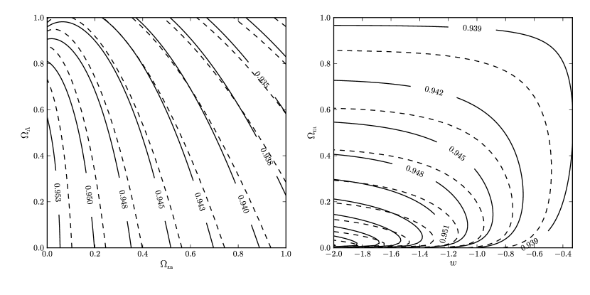
Figure 1: Isodensity contours for $\Xi({z_{\mathrm{1}}},{z_{\mathrm{2}}},\Omega)$ with source redshifts $({z_{\mathrm{1}}},{z_{\mathrm{2}}})=(1.5,2.5)$ (solid lines) and $({z_{\mathrm{1}}},{z_{\mathrm{2}}})=(2.0,3.0)$ (dashed lines) are shown in the plane $\Omega_{\mathrm{m}}-\Omega_{\mathrm{\Lambda}}$ with $w=-1$ (left panel) and $w-\Omega_{\mathrm{m}}$ with $\Omega_{k}=0$ (right panel). The redshift of the lens is ${z_{\mathrm{l}}}=0.2$. In the $\Omega_{\mathrm{m}}-\Omega_{\mathrm{\Lambda}}$ plane the contours nearly go in the direction of constant curvature $\Omega_{k}=1-\Omega_{\mathrm{m}}-\Omega_{\mathrm{\Lambda}}=\mathrm{constant}$. This implies that gravitational lensing is particularly sensitive to the curvature of the universe. Along the isodensity contours the cosmological information is completely degenerate, but one can break this degeneracy by adding probes with different source redshifts.

In the case of a single source plane, $\tilde{\kappa}$ is completely degenerate with the distance ratio $\Delta_{\mathrm{s}}$, since gravitational lensing is only able to infer $\kappa$ and both $\tilde{\kappa}$ and $\Delta_{\mathrm{s}}$ in Eq. (7) are unknown. Consequently, we can not constrain the cosmological parameters $\Omega$ contained in $\Delta_{\mathrm{s}}$ by exploiting only a single image system. Additional information on the cluster mass distribution is needed to break the degeneracy between $\tilde{\kappa}$ and $\Delta_{\mathrm{s}}$. This information is, for example, given by dynamical analyses from optical observations of the velocity dispersion of the cluster galaxies (e.g., Wojtak et al., 2007), or from X-ray observations which reveal the luminosity, temperature, and location of the intracluster medium (e.g., Vikhlinin et al., 2006).

The information from additional image systems can break this degeneracy, too. By means of a second source plane at redshift $z_{2}$ gravitational lensing infers $\kappa(z_{2})$. Combining inferences from two source planes at the redshifts $z_{1}$ and $z_{2}$ one obtains

$$\frac{\kappa(z_{1})}{\kappa(z_{2})}=\frac{\Delta_{\mathrm{1}}(\Omega)}{\Delta_{\mathrm{2}}(\Omega)}=:\Xi(z_{1},z_{2},\Omega),$$ (8)

where the dependency on the cosmological parameters $\Omega$ is explicitly given. This ratio does not depend on the lens mass distribution $\tilde{\kappa}$. By comparing image positions of lensed sources at different redshifts we can then construct a cosmological probe based on the ratio of distance ratios $\Xi(z_{1},z_{2},\Omega)$. Figure 1 shows the isodensity contours of $\Xi({z_{\mathrm{1}}},{z_{\mathrm{2}}},\Omega)$ for different redshift values in the $\Omega_{\mathrm{m}}-\Omega_{\mathrm{\Lambda}}$ plane, as well as in the $w-\Omega_{\mathrm{m}}$ plane, where a flat universe is assumed. The cosmological information is completely degenerate along the contours, where the value for $\Xi$ is constant. We can break this degeneracy by combining data from three or more source planes.

In the left panel the degeneracy nearly goes in the direction of constant curvature, meaning that gravitational lensing is particularly sensitive to the curvature of the universe.

2.2 Hidden priors

The laws governing gravitational lensing are invariant under specific transformations of some observables, whose physical features by contrast are not (Gorenstein et al., 1988; Saha, 2000). This leads to parameter degeneracies when interpreting observations and inferring physical parameters. In gravitational lensing, all observables except for the time delay are dimensionless, and the inference of $\kappa$ is invariant under the renormalization by an arbitrary constant $\mu$ of the angles $\boldsymbol{\theta}$ and $\boldsymbol{\beta}$. This implies that the inference of the $\Delta_{\mathrm{s}}$’s does not depend on the radial position of the images, but only on their relative geometrical distribution.

Another relevant degeneracy is the so called mass-sheet (or steepness) degeneracy (Schneider & Sluse, 2013), where the corresponding transformation with an arbitrary constant $\mu$ is

$$\boldsymbol{\beta}\longrightarrow\mu\boldsymbol{\beta};\quad(1-\kappa)\longrightarrow\mu(1-\kappa).$$ (9)

Although the image structure remains the same, the inferred mass profile changes, since this transformation rescales $\kappa$ by $\mu$ and adds or subtracts the constant mass sheet $(1-\mu)$ to the lens. This implies that the steepness of the mass profile is degenerate with the unknown source position when exploiting a single redshift image system.

There are many ways in which one can break the mass-sheet degeneracy (Saha, 2000). In our case, as there is little chance to measure the time delays of the images or the source absolute magnitude, we can break the degeneracy by again exploiting a second image system. Sources at different redshifts imply different lens equations (1). These equations are then no more simultaneously invariant under the transformation in Eq. (9), implying that the profile steepness is constrained by $\Xi({z_{\mathrm{1}}},{z_{\mathrm{2}}},\Omega)$ in Eq. (8).

Under the variation of $\Omega$, the values for the distance ratios $\Delta_{\mathrm{s}}$’s change, and consequently also the inferred steepness. In other words, when the cosmological parameters are set free, the mass-sheet degeneracy cannot be completely broken by exploiting multiple source redshifts. A degeneracy between the profile steepness and the cosmological parameters $\Omega$ still remains.

The typical approach when modeling gravitational lenses is to assume parametric models, which require a functional form for the mass profile that is in general not invariant under the transformation in Eq. (9). This assumption breaks the mass-sheet degeneracy even if the cosmological parameters are set free and therefore leads to unwanted priors when inferring the cosmological parameters, which may have a significant influence on the estimate of the cosmological parameters or at least on their uncertainties.

The inner density slope may vary from cluster to cluster and the best theoretical prediction for it is still debated (Limousin et al., 2012; Newman et al., 2013). Thus in order to make use of parametric models in the context of cosmological parameter determination a proper analysis should be devoted to the mass-sheet degeneracy. Considerable effort has been made to break this degeneracy when modelling and reconstructing the mass distribution of galaxies and galaxy clusters from gravitational lensing observations (e.g., Suyu et al., 2012; Collett et al., 2013; Greene et al., 2013; Umetsu, 2013). Making use of a non-parametric cluster mass description Bradač et al. (2004, 2005) combined weak and strong lensing to reconstruct the cluster mass profile and break the mass-sheet degeneracy. In the analysis of time-delay galaxies, Suyu et al. (2010, 2013) broke degeneracies by complementing lensing data with additional information that constrains the lens mass profile, such as the measurements of the stellar velocity dispersion or the mass distribution along the line of sight.

To avoid a biased inference a detailed analysis of the lens, exploiting observations other than strong gravitational lensing, is required in parametric models. We take an alternative approach and consider the more flexible free-form modeling of gravitational lenses to determine the cosmological parameters exploiting strong lensing observations alone.

3 Free-form lens modeling

For a general mass distribution the inversion problem of the lens equation (1) cannot be solved analytically but needs to be treated numerically. Moreover, in free-form reconstruction of gravitational lenses one has to deal with a much higher number of parameters than in parametric models. Crucially, however, the relationship between $\boldsymbol{\alpha}$ and $\kappa$ in Eq. (2) is linear due to the weak field limit of gravitational lensing (Schneider et al., 1992). We can therefore discretize the mass distribution into grid cells, or pixels, with constant convergence $\kappa_{i}$ and rewrite Eq. (1) for the $j^{\mathrm{th}}$ image at redshift $z_{j}$ as

$$\Delta_{j}\tilde{\boldsymbol{\beta}}_{j}=\boldsymbol{\theta}_{j}-\Delta_{j}\sum_{i}\tilde{\kappa}_{i}\tilde{\boldsymbol{\alpha}}_{i}(\boldsymbol{\theta}_{j}),$$ (10)

where $\Delta_{j}\tilde{\kappa}_{i}\tilde{\boldsymbol{\alpha}}_{i}(\boldsymbol{\theta}_{j})$ is the contribution to $\boldsymbol{\alpha}$ of the $i^{\mathrm{th}}$ pixel, $\tilde{\boldsymbol{\beta}}_{j}=\boldsymbol{\beta}_{j}(\Delta_{j})^{-1}$, and for all images of the same source the $\tilde{\boldsymbol{\beta}}_{j}$’s and $\Delta_{j}$’s are equal. This approach has been followed by Saha & Williams (2004) and Coe et al. (2008). Relations in the form of Eq. (10) for $p$ observed images construct a system of $2p$ linear equations

$${\bf A}x=b,$$ (11)

where ${\bf A}\in\mathbb{R}^{2p\times n}$, $b\in\mathbb{R}^{2p}$ is the constant vector of the $\boldsymbol{\theta}_{j}(\Delta_{j})^{-1}$, and $x\in\mathbb{R}^{n}$ is the vector containing the $n$ free parameters $\tilde{\kappa}_{i}$ and $\tilde{\boldsymbol{\beta}}_{j}$. This system is underdetermined as in general $2p\ll n$. Thus the solution space of Eq. (11) is unbounded and we need additional constraints to obtain a non-empty compact solution set. Moreover, some of these solutions are unphysical and have to be excluded.

Together with the constraints on the image positions, we require that the mass profile is well-behaved, i.e. non negative and smooth (Coles, 2008). These simple priors limit the solution space to a finite and physical set. To still maintain the linearity, we impose physically motivated constraints on the problem in the form of a system of $m$ linear inequalities

$${\bf C}x\leq d,$$ (12)

where ${\bf C}\in\mathbb{R}^{m\times n}$, and $d\in\mathbb{R}^{m}$ is a constant vector.

We take linear constraints, which impose that (i) the mass must be positive everywhere, (ii) its variations must be smooth, and (iii) the local density gradient must point within $45^{\circ}$ of the center. In addition, (iv) the arrival time order as well as the parity of the images are considered. The conditions (i) and (iv) are trivial requirements to ensure a positive mass density, where the produced images are located at the correct stationary points of the arrival time surface. The astrophysically motivated conditions (ii) and (iii) are required to exclude solutions, which mathematically satisfy the equations but are manifestly unphysical. The smoothness of the profile is achieved by imposing that the density of a pixel be no more than twice the average density of its neighbors (Coles, 2008), whereas the condition on the local density gradient guarantees an overall decaying mass density profile.

These criteria are weak and cannot drive the derivation of the mass profile, which is determined by the constraints on the image positions. They only ensure the solutions space to be bounded by requiring the mass density to satisfy some basic physical requirements. Moreover, they have been tested against either synthetic lenses from $N$-body and hydro simulations (Saha et al., 2006; Saha & Read, 2009) or toy models following NFW, power-law or isothermal profiles (Sereno & Zitrin, 2012; Lubini & Coles, 2012). It is consistently found that as long as the number of multiple images is large enough, the mass profile is determined by the data alone whereas the priors have only a role in the sampling strategy. An exhaustive discussion and a proper mathematical description of the assumed priors can be found in Coles (2008).

It is important to notice that we deliberately excluded any prior constraints on the steepness of the mass profile. Excluding such constraints is crucial to avoid uncontrolled priors on the cosmological parameters, because the steepness of the mass profile degenerates with cosmological parameters (see Section 5).

The solution set of Eq. (12) is then a subset of $\mathbb{R}^{n}$, which is bounded by the $m$ hyperplanes representing the constraints. On the other hand, the solution set of Eq. (11) is an affine space of $\mathbb{R}^{n}$ having dimension ${n_{\mathrm{dof}}}=n-2p$. Hence, the solution set of our problem is given by the intersection between these two sets, which constructs a non-empty convex polytope $S$, or simplex, embedded in the affine space. Eq. (11) therefore serves to reduce the dimension of the problem from $n$ to ${n_{\mathrm{dof}}}$.

We are interested in finding the volume of the simplex $S$. As this is in general not possible, we will derive the volume from an uncorrelated random sample $X$ drawn uniformly from $S$ (see Section 4). These parameter spaces, however, are typically embedded in 100 or more dimensions, and therefore the sampling becomes numerically challenging. To obtain an uncorrelated sample $X$ of points in $S$ we use the gravitational lens modeling framework GLASS (Lubini & Coles, 2012, Coles et al. in prep.), which is designed for free-form lens modeling. GLASS uses an MCMC method based on the Metropolis-Hasting algorithm (Metropolis et al., 1953; Hastings, 1970) with a symmetric proposal density function, which uses Eq. (12) to hint at the shape of $S$. This allows efficient sampling of the parameter space $S$ despite the high-dimensionality. The algorithm gives an uncorrelated random sample $X$, whose distribution is as good as an uniform random sample of $S$ (Lubini & Coles, 2012).

4 Method

4.1 Occam’s razor

The method we propose to infer the probability distribution of the cosmological parameters in strong gravitational lensing observations employs a Bayesian approach for model comparison. A standard method to estimate the cosmological parameters $\Omega$ is to append them to the vector of the free parameters $x$ and fit all the parameters together by maximizing the likelihood function. In order to be able to find a best fit, however, more data points than parameters are needed. This is possible in the case of parametric models, as in general the number of image position coordinates is larger than the number of free model parameters. The problem is therefore overdetermined and cannot be solved exactly, but the maximum of the likelihood function can be found. At a first level of inference, assuming flat priors, the probability distribution of the parameters $\Omega$ is then given by the likelihood function marginalized over the other model parameters $x$.

In our case the number of parameters is much larger than the data points. Hence, the number of solutions is infinite, i.e. all $x\in S$ exactly solve Eq. (1) and have the same likelihood with $\chi^{2}=0$. We are therefore not able to determine the best fit parameters using Bayesian first level inference. At the second level of inference, we can estimate the plausibility of different models given the data, even in an underdetermined case. This is possible because of the Bayesian Occam’s razor for model comparison (Mackay, 2003), where the plausibility of a model is proportional to the volume occupied by $S$ in the parameter space.

The Occam factor for the cosmological parameters in free-form lens modeling is derived as follows. Let us consider different gravitational lens mass reconstruction models $\mathcal{M}_{l}$ which reproduce the data $\mathcal{D}$ given by the image positions, each time assuming different values $\Omega_{l}$ for the cosmological parameters. The model $\mathcal{M}_{l}$ is then described by the cosmological parameters and the setting parameters defining the discretized convergence map. The free parameters $x$ of these models are the mass of the pixels and the source position coordinates, whereas the posterior probability of our problem is given by Bayes’ theorem as

$$P(x|\mathcal{D},\mathcal{M}_{l})=\frac{P(\mathcal{D}|x,\mathcal{M}_{l})P(x|\mathcal{M}_{l})}{P(\mathcal{D}|\mathcal{M}_{l})}.$$ (13)

Assuming flat priors for the models, which means that $P(\mathcal{M}_{l})$ is constant, the probability of a model given the data is proportional to the evidence $P(\mathcal{D}|\mathcal{M}_{l})$ in Eq. (13). Marginalizing over $x$ we obtain

$$P(\mathcal{M}_{l}|\mathcal{D})\propto P(\mathcal{D}|\mathcal{M}_{l})=\int_{\mathbb{R}^{n}}\!\!P(\mathcal{D}|x,\mathcal{M}_{l})P(x|\mathcal{M}_{l})\mathrm{d}x.$$ (14)

On the one hand, the prior $P(x|\mathcal{M}_{l})$ can be obtained considering Eqs. (11) and (12), and assuming that the data $\mathcal{D}$, i.e. the positions of the images, are unknown (see Section 4.2). These equations define the region $R_{l}\subset\mathbb{R}^{n}$, in which $x$ is allowed a priori by the model $\mathcal{M}_{l}$ before the data arrive. Since only for $x\in R_{l}$ these equations are exactly satisfied, the prior $P(x|\mathcal{M}_{l})$ is uniform in $R_{l}$ and vanishes outside. That means for $x\in R_{l}$

$$P(x|\mathcal{M}_{l})=1/V(R_{l}),$$ (15)

where $V(R_{l})$ is the volume of $R_{l}$. On the other hand, since only for $x\in S_{l}\subset R_{l}$ the data $\mathcal{D}$ are exactly reproduced by the model $\mathcal{M}_{l}$, the likelihood reads

$$P(\mathcal{D}|x,\mathcal{M}_{l})=\left\{\begin{array}[]{l}1\quad\text{if}\ x\in S_{l}\\ 0\quad\text{if}\ x\not\in S_{l}\end{array}\right..$$ (16)

From Eqs. (15) and (16) the evidence in Eq. (14) can be reduced to

$$P(\mathcal{D}|\mathcal{M}_{l})=\int_{S_{l}}P(x|\mathcal{M}_{l})\mathrm{d}x=\frac{V(S_{l})}{V(R_{l})}.$$ (17)

This ratio is called the Occam factor and it is the ratio between the posterior and the prior accessible volume in the parameter space (Mackay, 2003). As the purpose of this paper is to obtain confidence levels for the cosmological parameters, we are only interested in the Bayes factor

$$\frac{P(\mathcal{M}_{1}|\mathcal{D})}{P(\mathcal{M}_{2}|\mathcal{D})}=\frac{V(S_{1})\,V(R_{2})}{V(S_{2})\,V(R_{1})},$$ (18)

where the probabilities of the models assuming either $\Omega_{1}$ or $\Omega_{2}$ are compared. Assumptions causing a small collapse of the space volume after the data arrive, i.e. high Occam factor, are favored compared to the one having a larger collapse (Mackay, 2003). Thus we estimate the plausibility of the parameters $\Omega$ by means of Eq. (18), where the volumes of $S$ and $R$ have to be computed.

4.2 Probability computation

Computing the volumes of such simplices, however, is not without its own problems, since it has been shown that computing the exact volume of a convex polytope is #P-hard, even if all its vertices are known (Dyer & Frieze, 1988). We are therefore not able to compute $V(S)$ in high-dimensions, because the number of vertices has a huge combinatorial upper bound (McMullen & Shephard, 1971). An approximation of $V(S)$ is therefore needed. As we are only interested in ratios between volumes in Eq. (18), the volume of a simplex can be well approximated by means of its covariance matrix ${\bf\Sigma}$ through

$$V(S)\simeq\sqrt{\det{\bf\Sigma}}=\prod_{i=1}^{n_{\mathrm{dof}}}\sqrt{\lambda_{i}},$$ (19)

where $\lambda_{i}$ are the eigenvalues of ${\bf\Sigma}$. This means that we approximate the true volume $V(S)$ with the volume of an ${n_{\mathrm{dof}}}$-dimensional ellipsoid or hyperrectangle, whose axis lengths correspond to the square root of the eigenvalues of ${\bf\Sigma}$.

To estimate ${\bf\Sigma}$ we use the covariance matrix $\widehat{{\bf\Sigma}}$ of a sample of points $X$ uniformly and randomly distributed in $S$, which, as detailed in Section 3, we achieve using the program GLASS. Since the simplex $S$, and therefore also $X$, are embedded in a ${n_{\mathrm{dof}}}$-dimensional affine space, the matrix $\widehat{{\bf\Sigma}}\in\mathbb{R}^{n\times n}$ is singular, and all the $n-{n_{\mathrm{dof}}}=2p$ eigenvalues of $\widehat{{\bf\Sigma}}$, whose eigenvectors are perpendicular to the affine space, vanish. The sample size $|X|$ has accordingly to be $\geq{n_{\mathrm{dof}}}+1$, and the points of $X$ must not lie on the same $({n_{\mathrm{dof}}}-1)$-dimensional hyperplane of $\mathbb{R}^{n}$, meaning that ${n_{\mathrm{dof}}}$ eigenvalues of $\widehat{{\bf\Sigma}}$ have to be strictly positive. Moreover, to reasonably estimate ${\bf\Sigma}$, samples with $|X|\gg{n_{\mathrm{dof}}}$ are needed. When too few points are used, especially in high dimensions, the product in Eq. (19) will have a huge statistical uncertainty due to the randomness of the sampling.

As already stated above, the prior accessible volume $V(R)$ is given considering Eqs. (11) and (12), and assuming $\mathcal{D}$ to be unknown. $V(R)$ simply reflects the degeneracy in Eq. (7), i.e. the fact that the smaller the distance ratios $\Delta_{\mathrm{s}}$, the larger the value of the convergence $\tilde{\kappa}$, and, finally, the larger $V(R)$. On the one hand, in Eq. (12) the constraints on the arrival time and the parity are unknown, whereas the remaining constraints, which consist of the smoothness constraints of the mass distribution, the constraints on the local gradient, and $\kappa_{i}\geq 0$, can all be written in the form $c\cdot x\leq 0$, where $c$ is a constant vector. Therefore, the solution set is bounded by hyperplanes passing through the origin of the parameter space. Hence, these constraints do not depend on the norm $\|x\|$, which implies that the model dependent part of Eq. (12) constrains only the solid angle of $R$. This is shown schematically as the gray region in Figure 2. It is important to notice that only the information obtained from lensing observations and not the additional constraints of Eq. (12) constrain the norm $\|x\|$ and thus the mass of the pixels.

Figure 2: The prior accessible volume $V(R)$ is shown schematically for two different cosmological parameter assumptions $\Omega_{\mathrm{1}}$ and $\Omega_{\mathrm{2}}$. Here a 2-dimensional graph is shown for simplicity, where $x=(\kappa_{i},\kappa_{j})$. Equation ${\bf C}x\leq 0$ constrains the solid angle of $R$, whereas equation ${\bf A}x=b$ defines the affine solution space. The only $\Omega$ dependent part in these two equations is the vector $b$. The volumes $V(R_{1})$ and $V(R_{2})$ are then proportional to $d_{1}=\|{\bf A}^{-1}\,b_{1}\|$ and $d_{2}=\|{\bf A}^{-1}\,b_{2}\|$, since in this case ${n_{\mathrm{dof}}}=1$.

On the other hand, as the unknown data imply unknown $\boldsymbol{\theta}$ and ${\bf A}$, the solution set of Eq. (11) is an affine space with unknown angular position. The solid angle as well as the angular position of $R$ do not depend on $\Omega$ and are therefore equal for all $\mathcal{M}$. The only cosmological parameter dependent part in these equations is given by the vector $b$ in Eq. (11), since its components are proportional to $\Delta_{j}(\Omega)^{-1}$. The distance $d$ between the affine space and the origin of the parameter space is defined by $b$ through

$$d=\|{\bf A}^{-1}\,b\|,$$ (20)

where ${\bf A}^{-1}$ denotes the Moore-Penrose pseudoinverse of ${\bf A}$. Since $\boldsymbol{\theta}$ and ${\bf A}$ are unknown we assume random values for their components, implying that

$$d\,\mathrel{\raisebox{4.0pt}{$\sim$}\hbox{$\propto$}}\langle\Delta_{j}(\Omega)^{-1}\rangle,$$ (21)

where $\langle\,\cdot\,\rangle$ is the arithmetic mean over the images $j$. For the probability ratio in Eq. (18) it is enough to consider the cosmological parameter dependent part, which for the volume of $R$ is given by

$$V(R)\propto d^{n_{\mathrm{dof}}}\propto\mathcal{H}(\Delta_{j}(\Omega_{l}))^{-{n_{\mathrm{dof}}}},$$ (22)

where $\mathcal{H}(\,\cdot\,)$ is the harmonic mean over the images $j$. Figure 2 shows schematically the volumes $V(R_{1})$ and $V(R_{2})$ obtained considering two different affine spaces, where the vectors $b_{1}$ and $b_{2}$ correspond to $\Omega_{1}$ or $\Omega_{2}$, respectively. The volumes are then proportional to $d_{1}^{n_{\mathrm{dof}}}$ and $d_{2}^{n_{\mathrm{dof}}}$. In this example ${n_{\mathrm{dof}}}=1$, since for simplicity we show a 2-dimensional plot.

Considering Eqs. (19) and (22), we obtain the final estimate for the probability of a cosmological model $\mathcal{M}_{l}$ given the data $\mathcal{D}$, which reduces to

$$P(\mathcal{M}_{l}|\mathcal{D})\propto\left(\prod_{i=1}^{{n_{\mathrm{dof}}}}\sqrt{\widehat{\lambda}_{l,i}}\right)\cdot\mathcal{H}(\Delta_{j}(\Omega_{l}))^{n_{\mathrm{dof}}},$$ (23)

where $\widehat{\lambda}_{l,i}$ are the ${n_{\mathrm{dof}}}$ positive eigenvalues of $\widehat{{\bf\Sigma}}_{l}$. To better understand this result, let us consider the special case of a single source redshift ${z_{\mathrm{s}}}$. The harmonic mean then reduces to $\mathcal{H}(\Delta_{j}(\Omega_{l}))=\Delta_{\mathrm{s}}(\Omega_{l})$ and Eq. (10) can be rewritten in the variables $\kappa_{i}=\tilde{\kappa}_{i}\cdot\Delta_{\mathrm{s}}(\Omega_{l})$ and $\boldsymbol{\beta}_{j}=\tilde{\boldsymbol{\beta}}_{j}\cdot\Delta_{\mathrm{s}}(\Omega_{l})$ for all the images $j$. Thus the factor $\Delta_{\mathrm{s}}(\Omega_{l})$ cancels out in Eq. (10), which does not depend anymore on the choice of $\Omega_{l}$. The simplex $S_{l}$ in the $(\tilde{\kappa}_{i},\tilde{\boldsymbol{\beta}}_{j})$-space can be transformed in the corresponding simplex $S^{\prime}$ in the $(\kappa_{i},\boldsymbol{\beta}_{j})$-space simply by multiplying the coordinates with the factor $\Delta_{\mathrm{s}}(\Omega_{l})$. Hence, for Eq. (23) we obtain

$$P(\mathcal{M}_{l}|\mathcal{D})\propto V(S_{l})\cdot\Delta_{\mathrm{s}}(\Omega_{l})^{{n_{\mathrm{dof}}}}=V(S^{\prime}),$$ (24)

meaning that the probability is proportional to the volume of the simplex in the $(\kappa_{i},\boldsymbol{\beta}_{j})$-space. By construction, $V(S^{\prime})$ does not depend on the choice of $\Omega_{l}$, and thus neither does $P(\mathcal{M}_{l}|\mathcal{D})$. As expected from the discussion in Section 2, regarding the degeneracy in Eq. (7), we cannot constrain cosmological parameters with a single source plane.

In the case of multiple source redshifts, since $\kappa_{i}$ depends on the redshift of the source, there are many different $(\kappa_{i},\boldsymbol{\beta}_{j})$-spaces. Hence, instead of $V(S^{\prime})$ in Eq. (23) we have to consider an average of the volumes of the simplices in the $(\kappa_{i},\boldsymbol{\beta}_{j})$-spaces to be proportional to the probability. For this reason the factor $\mathcal{H}(\Delta_{j}(\Omega_{l}))^{n_{\mathrm{dof}}}$ is required in Eq. (23), and thus it accounts for the degeneracy in Eq. (7).

5 Tests

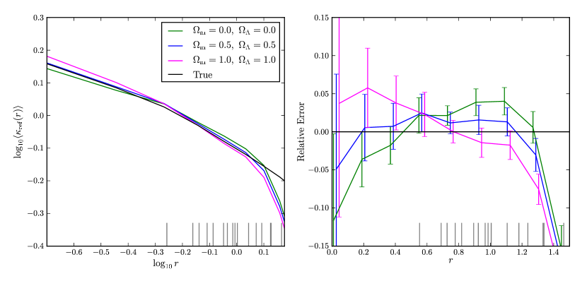
Figure 3: Left panel: The reconstructed lens profile ${\kappa_{\mathrm{ref}}}$ (${z_{\mathrm{ref}}}=2$) of the same lens are shown for three different sets of cosmological parameters. Only the assumed values for $\Omega=(\Omega_{\mathrm{m}},\Omega_{\mathrm{\Lambda}})$ change between the reconstructions. $\langle{\kappa_{\mathrm{ref}}}(r)\rangle$ is the mean of ${\kappa_{\mathrm{ref}}}$ within the pixelated ring of radius $r$, which is in units of $\langle\|\boldsymbol{\theta}_{j}\|\rangle$. The images, whose positions are marked by gray lines, are located at radii $0.55\leq r\leq 1.46$, or $-0.26\leq\log_{10}r\leq 0.16$. For comparison the true mass profile, used to produce the image systems under the assumption of $\Omega_{\mathrm{ref}}=(0.5,0.5)$, is shown in black. The fits are not physical outside the outermost images, since there is no lensing information on the mass profile. Right panel: To highlight the degeneracy between steepness and cosmological parameters, the relative error with respect to the true mass profile ${\kappa_{\mathrm{ref}}}/\kappa_{\mathrm{true}}-1$ is shown. The three curves in the plot have been slightly shifted to avoid the overlapping of the $1\sigma$ error bars.

We test our method by means of synthetic lenses produced with Gravlens (Keeton, 2001a, b). This software builds lenses as parametric mass distributions and finds, through numerical inversion of the lens equation (1), the position, the arrival time, and the parity of all the images produced by a given source position. Image configurations $\mathcal{D}$ are produced by the synthetic lenses assuming a reference set of true cosmological parameters $\Omega_{\mathrm{ref}}$. This is a realistic testing procedure, since our method utilizes a discretized mass distribution, whereas the adopted image configurations are obtained from smooth lenses, just as real galaxies or galaxy clusters. For simplicity and without loss of generality we renormalize each image position $\boldsymbol{\theta}$ by the mean radius $\langle\|\boldsymbol{\theta}_{j}\|\rangle$ of all the images. This leaves the results unchanged (see Section 2) and allows for an easier comparison between different configurations and mass profiles.

For each cosmological model, by means of GLASS, we then find a set $X$ of discretized mass distributions and source positions, i.e. $x\in S_{l}$, which exactly reproduce the synthetic image configuration.

The discretized mass distribution is defined within a radius $R$, which is divided into $P$ pixels (Saha & Williams, 2004). Thus the models $\mathcal{M}_{l}$ depends not only on $\Omega_{l}$ but also on the model parameters $R$ and $P$. While the latter changes the resolution of the discretization, $R$ does not influence $n$. We fix $P$ a priori and marginalize over $R$, that is

$$P(\Omega_{l},\mathcal{M}|\mathcal{D})=\int_{\mathbb{R}}P(\Omega_{l},R,\mathcal{M}|\mathcal{D})\,\mathrm{d}R,$$ (25)

where the dependency on $\Omega_{l}$ and $R$ is written explicitly. The marginalization with respect to $R$ is important, since for different $\Omega_{l}$ the probabilities may have their maximum at different $R$’s. Moreover, this procedure enables us to exclude those image configurations where $P(\Omega_{l},R,\mathcal{M}|\mathcal{D})$ as a function of $R$ is not single peaked or heavily depends on the choice of $\Omega_{l}$. Without accounting for different map radii, cosmological information would be strongly affected by the discretization and thus no longer reliable.

To test the model, we consider a realistic scenario, where the lens located at redshift ${z_{\mathrm{l}}}=0.2$ is a massive cluster, that follows a single NFW profile with concentration parameter $c_{200}=5$, mass $M_{200}=10^{15}M_{\odot}/h$, and ellipticity $e=0.15$. To produce the synthetic image configurations in this section we assume the $\Lambda$CDM cosmological model with $\Omega_{\mathrm{ref}}=(\Omega_{\mathrm{m}},\Omega_{\mathrm{\Lambda}})=(0.5,0.5)$. Results for this reference cosmological model are then compared to two competitive models, the empty open universe $\Omega_{\mathrm{emp}}=(0,0)$ and a closed universe, $\Omega_{\mathrm{cld}}=(1,1)$.

As discussed in Section 2 the mass-sheet degeneracy is still there even exploiting multiple source redshifts and setting $\Omega$ free. We consider an image configuration with 5 different source planes producing overall 16 images, whose redshifts are ${z_{\mathrm{s}}}=1.0,\ 1.5,\ 2.0,\ 2.5$, and $3.0$, respectively. The mean mass profiles for the three fits are shown in Figure 3. The profile steepness depends on the assumed cosmological parameters. Cosmologies with a larger $\Omega_{k}$ need a shallower mass profile in order to fit the given configuration. The fit with the correct value for $\Omega$ excellently reproduces the true mass profile within the outermost image radius. Thus GLASS is able to reproduce the assumed profile and produces an unbiased mass estimate (Lubini & Coles, 2012).

Outside the outermost image position there is no information on the profile and the fits are unphysical. This is because in Eq. (12) we consider moderate constraints and let the steepness of the profile completely free to vary in order to avoid breaking any possible degeneracy as, for instance, the mass-sheet degeneracy. This issue, however, has no influence on our analysis, as these pixels are not constrained by the images and thus are independent of $\Omega_{l}$. Nevertheless, these pixels have to be considered, since otherwise the approximation $V(S)\simeq(\det\widehat{{\bf\Sigma}})^{1/2}$ in Eq. (19) is no longer valid.

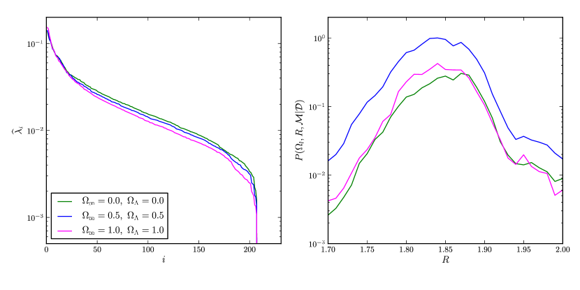
Figure 4: Left panel: The sorted list of the eigenvalues $\widehat{\lambda}_{i}$ of $\widehat{{\bf\Sigma}}$ for the three different fits with $|X|=10^{4}$ and $R=1.85$ are shown. The first ${n_{\mathrm{dof}}}=207$ eigenvalues are strictly positive, whereas the last $n-{n_{\mathrm{dof}}}=2p=24$ are not displayed, as they are $<10^{-14}$, which means $0$ within the machine precision. Right panel: The probability $P(\Omega_{l},R,\mathcal{M}|\mathcal{D})$ as a function of $R$ is shown for the three fits. The three curves were rescaled in arbitrary units. The blue curve corresponding to $\Omega_{\mathrm{ref}}$ is larger than the other two cases, meaning that this assumption is more likely.

We elucidate and test some properties of Eq. (23) by means of an image configuration with 3 sources producing overall $p=12$ images, i.e. 3 quads, whose source redshift are ${z_{\mathrm{s}}}=1.0$, $2.0$, and $3.0$, respectively. We produce solution sets $X$ with $|X|=10^{4}$ and $P=8$, which implies that there are $n=231$ free parameters. The sorted list of the eigenvalues $\widehat{\lambda}_{i}$ in the case with $R=1.85$ is shown in the left panel of Figure 4. Only the first ${n_{\mathrm{dof}}}=207$ eigenvalues are strictly positive, whereas the remaining $2p=24$ vanish, as expected. The larger eigenvalues correspond to the more massive pixels, i.e. those located in the very inner region of the mass distribution. The mass-sheet degeneracy is therefore also visible in the steepness of the curves of the three different cosmologies.

The right panel of Figure 4 shows $P(\Omega_{l},R,\mathcal{M}|\mathcal{D})$ as a function of $R$ for the three sets of cosmological parameters. The curves are single peaked with the maximum around $R=1.85$ and the curve corresponding to the true cosmological parameters has a larger normalization than the others. The marginalization over $R$ yields the probabilities $P(\Omega_{l},\mathcal{M}|\mathcal{D})$. The true cosmology is clearly favored with $P(\Omega_{\mathrm{ref}},\mathcal{M}|\mathcal{D})$ being about 3 times larger than $P(\Omega_{\mathrm{emp}},\mathcal{M}|\mathcal{D})$ and $P(\Omega_{\mathrm{cld}},\mathcal{M}|\mathcal{D})$.

We finally verified that the method is unbiased to the underlying cosmological model of reference. Even assuming the extreme case $\Omega_{\mathrm{ref}}=(\Omega_{\mathrm{m}},\Omega_{\Lambda})=(2.5,0.5)$ our method could find $\Omega_{\mathrm{ref}}$ within the uncertainties.

6 Parameter determination

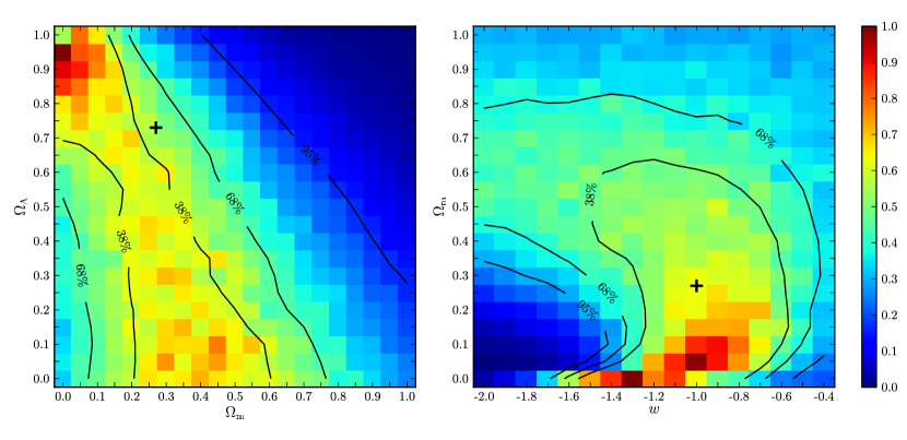
Figure 5: The inferred probability distribution for a single lensing cluster in the $\Omega_{\mathrm{m}}-\Omega_{\mathrm{\Lambda}}$ plane with $w=-1$ (left panel) and in the $w-\Omega_{\mathrm{m}}$ plane with $\Omega_{k}=0$ (right panel). The probability isodensity contours almost correspond to the contours shown in Figure 1 and the area enclosed by the contours corresponds to respectively $38\%$, $68\%$, and $95\%$ of the total probability. The true values for the cosmological parameters $\Omega_{\mathrm{ref}}=(0.27,0.73,-1)$ are shows by the black crosses.

To show the accuracy of the method, we considered the massive cluster with $(c_{200},M_{200},e)=(5,10^{15}M_{\odot}/h,0.15)$ of Section 5 and the concordance $\Lambda$CDM cosmology with $\Omega_{\mathrm{ref}}=(\Omega_{\mathrm{m}},\Omega_{\mathrm{de}},w)=(0.27,0.73,-1)$ (Komatsu et al., 2011) as the “true” cosmological model. The synthetic image configuration is produced by 5 sources at redshifts ${z_{\mathrm{s}}}=1.2$, $1.9$, $2.5$, $2.8$ and $4.0$, which produce three quads and two doubles. The total of 16 images at different redshifts contains the information on the cosmography.

We fit the parameters either in the $\Omega_{\mathrm{m}}-\Omega_{\mathrm{\Lambda}}$ plane, where $(\Omega_{\mathrm{m}},\Omega_{\mathrm{\Lambda}})\in[0,1]\times[0,1]$ with $w=-1$, or in the $w-\Omega_{\mathrm{m}}$ plane, where $(w,\Omega_{\mathrm{m}})\in[-2,-1/3]\times[0,1]$ and $\Omega_{k}=0$. We divided the two planes into grids, and computed the probabilities $P(\Omega_{l},\mathcal{M}|\mathcal{D})$ marginalizing over $R$ for each model $\Omega_{l}$.

Although the sampling algorithm has been recently improved, it still has a running time of $\mathcal{O}(n^{3})$ (Lubini & Coles, 2012). Thus, we need to keep the space dimension small enough to have a reasonable computation time, but large enough such that the discretization does not compromise the fit of the image configuration. For this reason we choose $P=8$, which corresponds to $n=235$, and divide the planes into grids of $21\times 21$ and $21\times 17$ pixels, respectively.

The results are shown for the $\Omega_{\mathrm{m}}-\Omega_{\mathrm{\Lambda}}$ plane in the left panel of Figure 5, and for the $w-\Omega_{\mathrm{m}}$ plane in the right panel. The probability isodensity contours follow those in Figure 1, since for gravitational lensing the information of the cosmological parameters is contained in $\Xi$. The parameter degeneracy is partially broken thanks to the multiple source redshifts.

The method is mainly sensitive to the space curvature parameter $\Omega_{k}$ and the matter density parameter $\Omega_{\mathrm{m}}$ in the $\Omega_{\mathrm{m}}-\Omega_{\mathrm{\Lambda}}$ plane, and to the dark energy equation of state $w$ in the $w-\Omega_{\mathrm{m}}$ plane. These parameters are almost perpendicular to the degeneracies in the respective planes, and can therefore be inferred by means of a single lens even if with large uncertainties.

Our method obtains an unbiased estimate of the assumed values for the cosmological parameters within the statistical uncertainties. $\Omega_{k}$ is retrieved with an accuracy of $0.3$ and $w$ with an uncertainty of about $0.4$, whereas $\Omega_{\mathrm{m}}$ is accurate within $0.3$.

7 Conclusions

Strong gravitational lensing exploiting multiple lensed background sources in galaxy clusters is a unique tool to probe the cosmology. It relies on purely geometrical information that does not need any calibration, and explores new redshift ranges around $z\sim 3-4$. To extract the cosmological information contained in lensed image systems, we exploited free-form lens modeling by means of the framework GLASS. This software is based on an efficient sampling strategy that produces uncorrelated random samples (Lubini & Coles, 2012). These are fundamental for our analysis, since the solution spaces we need to sample are convex polytopes in 200 and more dimensions.

The free-form approach we investigated is more flexible than parametric techniques, and requires only the geometrical information from strong lensing. Parametric models demand deep knowledge of all cluster components, and assume functional forms for the mass profiles, which break the mass-sheet degeneracy. When inferring the cosmological parameters, however, the mass-sheet degeneracy is still present even in the case of multiple source planes, since cosmologies with larger $\Omega_{k}$ need shallower mass profiles to fit the same image configuration. Therefore parametric models unintentionally break possible degeneracies by adding hidden priors to the analysis. This leads to biased estimates with unrealistically small uncertainties.

Our method does not use constraints on the steepness of the profile and accounts for the mass-sheet degeneracy. This solves one of the main systematics in lensing determination of cosmological parameters. The systematic effect due to the presence of uncorrelated substructures along the line of sight (D’Aloisio & Natarajan, 2011), which is a main source of uncertainty in cosmography, has not been considered in this paper. However, cosmic variance plays a minor role in the strong lensing regime.

Since in free-form modeling there are more free parameters than data points, we cannot follow a maximum-likelihood estimation of the cosmological parameter. Therefore, we developed a method based on Bayesian model comparison. The probabilities are obtained through the Occam factor, which means that we take the volume of the solution space as a tracer of the probability. We considered the probability to be proportional to the ratio between the posterior and prior accessible volumes.

Testing with synthetic lenses showed that our method can infer the values of the assumed cosmological parameters. The free-form strong lensing geometrical test we developed seems particularly promising in view of ongoing and future observational programs. The Cluster Lensing And Supernova survey with Hubble (CLASH) project (Postman et al., 2012) has been deeply observing 25 massive clusters at $0.2\lesssim z\lesssim 0.6$. Predictions and first analyses (Umetsu et al., 2012; Medezinski et al., 2013) agree on an expected detection rate of at least between $12$ and $15$ multiple systems per clusters. On the basis of the CLASH clusters alone, the strong lensing test we proposed might decrease the uncertainties of the cosmological parameters with respect to ones obtained for one single cluster in Section 6 by almost one order of magnitude.

Future surveys will provide additional very large cluster samples. Euclid is expected to detect about $5000$ clusters with prominent arcs and strong lensing features (Laureijs et al., 2011). The consequent improvement of the method accuracy over such a large sample is of one or two additional orders of magnitude. The performance should further improve using the method in combination with orthogonal probes such as CMB or BAO.

References

- Abdelsalam et al. (1998a) Abdelsalam H. M., Saha P., Williams L. L. R., 1998a, MNRAS, 294, 734
- Abdelsalam et al. (1998b) Abdelsalam H. M., Saha P., Williams L. L. R., 1998b, AJ, 116, 1541
- Amanullah et al. (2010) Amanullah R., Lidman C., Rubin D., Aldering G., Astier P., Barbary K., Burns M. S., Conley A., 2010, ApJ, 716, 712
- Bolton et al. (2008) Bolton A. S., Burles S., Koopmans L. V. E., Treu T., Gavazzi R., Moustakas L. A., Wayth R., Schlegel D. J., 2008, ApJ, 682, 964
- Bradač et al. (2004) Bradač M., Lombardi M., Schneider P., 2004, A&A, 424, 13
- Bradač et al. (2005) Bradač M., Schneider P., Lombardi M., Erben T., 2005, A&A, 437, 39
- Coe et al. (2008) Coe D., Fuselier E., Benítez N., Broadhurst T., Frye B., Ford H., 2008, ApJ, 681, 814
- Coles (2008) Coles J., 2008, ApJ, 679, 17
- Collett et al. (2013) Collett T. E., Marshall P. J., Auger M. W., Hilbert S., Suyu S. H., Greene Z., Treu T., Fassnacht C. D., Koopmans L. V. E., Bradač M., Blandford R. D., 2013, MNRAS, 432, 679
- D’Aloisio & Natarajan (2011) D’Aloisio A., Natarajan P., 2011, MNRAS, 411, 1628
- Deb et al. (2008) Deb S., Goldberg D. M., Ramdass V. J., 2008, ApJ, 687, 39
- Diego et al. (2005) Diego J. M., Sandvik H. B., Protopapas P., Tegmark M., Benítez N., Broadhurst T., 2005, MNRAS, 362, 1247
- Dyer & Frieze (1988) Dyer M. E., Frieze A. M., 1988, SIAM J. Comput., 17, 967
- Falco et al. (1985) Falco E. E., Gorenstein M. V., Shapiro I. I., 1985, ApJ, 289, L1
- Gilmore & Natarajan (2009) Gilmore J., Natarajan P., 2009, MNRAS, 396, 354
- Golse et al. (2002) Golse G., Kneib J.-P., Soucail G., 2002, A&A, 387, 788
- Gorenstein et al. (1988) Gorenstein M. V., Shapiro I. I., Falco E. E., 1988, ApJ, 327, 693
- Greene et al. (2013) Greene Z. S., Suyu S. H., Treu T., Hilbert S., Auger M. W., Collett T. E., Marshall P. J., Fassnacht C. D., Blandford R. D., Bradač M., Koopmans L. V. E., 2013, ApJ, 768, 39
- Hastings (1970) Hastings W. K., 1970, Biometrika, 57, 97
- Jullo et al. (2010) Jullo E., Natarajan P., Kneib J.-P., D’Aloisio A., Limousin M., Richard J., Schimd C., 2010, Science, 329, 924
- Keeton (2001a) Keeton C. R., 2001a, ArXiv Astrophysics e-prints
- Keeton (2001b) Keeton C. R., 2001b, ArXiv Astrophysics e-prints
- Komatsu et al. (2011) Komatsu E., Smith K. M., Dunkley J., Bennett C. L., Gold B., Hinshaw G., Jarosik N., Larson D., 2011, ApJS, 192, 18
- Laureijs et al. (2011) Laureijs R., Amiaux J., Arduini S., Auguères J.-L., Brinchmann J., Cole R., Cropper M., Dabin C., Duvet L., Ealet A., et al. 2011, ArXiv e-prints
- Liesenborgs et al. (2007) Liesenborgs J., de Rijcke S., Dejonghe H., Bekaert P., 2007, MNRAS, 380, 1729
- Limousin et al. (2012) Limousin M., Morandi A., Sereno M., Meneghetti M., Ettori S., Bartelmann M., Verdugo T., 2012, ArXiv e-prints
- Limousin et al. (2007) Limousin M., Richard J., Jullo E., Kneib J.-P., Fort B., Soucail G., Elíasdóttir Á., Natarajan P., Ellis R. S., Smail I., Czoske O., Smith G. P., Hudelot P., Bardeau S., Ebeling H., Egami E., Knudsen K. K., 2007, ApJ, 668, 643
- Lubini & Coles (2012) Lubini M., Coles J., 2012, MNRAS, 425, 3077
- Mackay (2003) Mackay D. J. C., 2003, Information Theory, Inference and Learning Algorithms. Cambridge University Press, Cambridge
- McMullen & Shephard (1971) McMullen P., Shephard G. C., 1971, Convex polytopes and the upper bound conjecture. Cambridge University Press, London
- Medezinski et al. (2013) Medezinski E., Umetsu K., Nonino M., Merten J., Zitrin A., Broadhurst T., Donahue M., Sayers J., Waizmann J.-C., Koekemoer A., Coe D., Molino A., Melchior P., Mroczkowski T., Czakon N., Postman M., 2013, ArXiv e-prints
- Metropolis et al. (1953) Metropolis N., Rosenbluth A. W., Rosenbluth M. N., Teller A. H., Teller E., 1953, J. Chem. Phys., 21, 1087
- Navarro et al. (1996) Navarro J. F., Frenk C. S., White S. D. M., 1996, ApJ, 462, 563
- Navarro et al. (1997) Navarro J. F., Frenk C. S., White S. D. M., 1997, ApJ, 490, 493
- Newman et al. (2013) Newman A. B., Treu T., Ellis R. S., Sand D. J., Nipoti C., Richard J., Jullo E., 2013, ApJ, 765, 24
- Percival et al. (2010) Percival W. J., Reid B. A., Eisenstein D. J., Bahcall N. A., Budavari T., Frieman J. A., Fukugita M., Gunn J. E., 2010, MNRAS, 401, 2148
- Planck Collaboration et al. (2013) Planck Collaboration Ade P. A. R., Aghanim N., Armitage-Caplan C., Arnaud M., Ashdown M., Atrio-Barandela F., Aumont J., Baccigalupi C., Banday A. J., et al. 2013, ArXiv e-prints
- Postman et al. (2012) Postman M., Coe D., Benítez N., Bradley L., Broadhurst T., Donahue M., Ford H., Graur O., Graves G., Jouvel S., Koekemoer A., Lemze D., Medezinski E., Molino A., Moustakas L., Ogaz S., 2012, ApJS, 199, 25
- Read et al. (2007) Read J. I., Saha P., Macciò A. V., 2007, ApJ, 667, 645
- Richard et al. (2009) Richard J., Pei L., Limousin M., Jullo E., Kneib J. P., 2009, A&A, 498, 37
- Riess et al. (2011) Riess A. G., Macri L., Casertano S., Lampeitl H., Ferguson H. C., Filippenko A. V., Jha S. W., Li W., Chornock R., 2011, ApJ, 730, 119
- Saha (2000) Saha P., 2000, AJ, 120, 1654
- Saha et al. (2006) Saha P., Coles J., Macciò A. V., Williams L. L. R., 2006, ApJ, 650, L17
- Saha & Read (2009) Saha P., Read J. I., 2009, ApJ, 690, 154
- Saha & Williams (2004) Saha P., Williams L. L. R., 2004, AJ, 127, 2604
- Schneider et al. (1992) Schneider P., Ehlers J., Falco E. E., 1992, Gravitational Lenses. Springer-Verlag, Berlin
- Schneider et al. (2006) Schneider P., Kochanek C., Wambsganss J., 2006, Gravitational Lensing: Strong, Weak and Micro. Springer-Verlag, Berlin
- Schneider & Sluse (2013) Schneider P., Sluse D., 2013, ArXiv e-prints
- Sereno (2002) Sereno M., 2002, A&A, 393, 757
- Sereno et al. (2013) Sereno M., Ettori S., Umetsu K., Baldi A., 2013, MNRAS, 428, 2241
- Sereno & Longo (2004) Sereno M., Longo G., 2004, MNRAS, 354, 1255
- Sereno et al. (2010) Sereno M., Lubini M., Jetzer P., 2010, A&A, 518, A55
- Sereno & Zitrin (2012) Sereno M., Zitrin A., 2012, MNRAS, 419, 3280
- Soucail et al. (2004) Soucail G., Kneib J.-P., Golse G., 2004, A&A, 417, L33
- Suyu et al. (2013) Suyu S. H., Auger M. W., Hilbert S., Marshall P. J., Tewes M., Treu T., Fassnacht C. D., Koopmans L. V. E., Sluse D., Blandford R. D., Courbin F., Meylan G., 2013, ApJ, 766, 70
- Suyu et al. (2012) Suyu S. H., Hensel S. W., McKean J. P., Fassnacht C. D., Treu T., Halkola A., Norbury M., Jackson N., Schneider P., Thompson D., Auger M. W., Koopmans L. V. E., Matthews K., 2012, ApJ, 750, 10
- Suyu et al. (2010) Suyu S. H., Marshall P. J., Auger M. W., Hilbert S., Blandford R. D., Koopmans L. V. E., Fassnacht C. D., Treu T., 2010, ApJ, 711, 201
- Umetsu (2013) Umetsu K., 2013, ApJ, 769, 13
- Umetsu et al. (2012) Umetsu K., Medezinski E., Nonino M., Merten J., Zitrin A., Molino A., Grillo C., Carrasco M., Donahue M., Mahdavi A., Coe D., Postman M., Koekemoer A., Czakon N., Sayers J., Mroczkowski T., 2012, ApJ, 755, 56
- Vikhlinin et al. (2006) Vikhlinin A., Kravtsov A., Forman W., Jones C., Markevitch M., Murray S. S., Van Speybroeck L., 2006, ApJ, 640, 691
- Voit (2005) Voit G. M., 2005, Reviews of Modern Physics, 77, 207
- Weinberg (1972) Weinberg S., 1972, Gravitation and Cosmology: Principles and Applications of the General Theory of Relativity. Wiley, New York
- Wojtak et al. (2007) Wojtak R., Łokas E. L., Mamon G. A., Gottlöber S., Prada F., Moles M., 2007, A&A, 466, 437
- Zieser & Bartelmann (2012) Zieser B., Bartelmann M., 2012, ArXiv e-prints