Quantum simulation of correlated-hopping models with fermions in optical lattices

Abstract

By using a modulated magnetic field in a Feshbach resonance for ultracold fermionic atoms in optical lattices, we show that it is possible to engineer a class of models usually referred to as correlated-hopping models. These models differ from the Hubbard model in exhibiting additional density-dependent interaction terms that affect the hopping processes. In addition to the spin-SU(2) symmetry, they also possess a charge-SU(2) symmetry, which opens the possibility of investigating the $\eta$-pairing mechanism for superconductivity introduced by Yang for the Hubbard model. We discuss the known solution of the model in 1D (where $\eta$ states have been found in the degenerate manifold of the ground state) and show that, away from the integrable point, quantum Monte Carlo simulations at half filling predict the emergence of a phase with coexisting incommensurate spin and charge order.

I Introduction.

The use of ultracold atoms in optical lattices as condensed matter simulators has brought a major advance in physics in the last decade. Both bosonic jaksch ; greiner and fermionic hofstetter ; esslinger Hubbard models have been theoretically and experimentally investigated, and the simulation of artificial gauge fields dalibard ; lihking and Quantum Hall physics aidelsburg ; miyake ; wouter are some of the many phenomena that this active field is unveiling lewenstein ; bloch1 ; bloch2 .

The realization of the fermionic Hubbard model opens the possibility of using quantum simulators to treat strongly-correlated fermionic systems, with the ultimate goal of understanding high-$T_{c}$ superconductivity. While it is more challenging to cool fermionic systems than bosonic ones, state-of-the-art techniques have recently allowed fermionic atoms to be cooled sufficiently to reach the regime where quantum magnetism manifests esslinger2 .

A particular interest with ultracold gases is the use of time-dependent driving potentials. Using this technique, it has been possible to observe the transition from a Mott-insulator to a superfluid phase in the Bose-Hubbard model by a dynamical suppression of tunneling eckardt2005 ; creffield ; lignier2007 , as well as the simulation of frustrated classical magnetism eckardt2010 ; struck2011 , and schemes for the realization of abelian struck2012 and non-abelian gauge fields hauke2012 . More recently, a time-dependent modulation of Feshbach resonances has been proposed for a system of ultracold bosons, leading to a model with density-dependent hopping coefficients, and exotic phenomena like pair superfluidity, and holon and doublon condensation rapp2012 .

In this paper we extend this idea to fermionic atom systems. We show how a time-dependent manipulation of the interaction strength allows us to simulate an unusual class of “correlated-hopping models” FF , opening a window for the experimental observation of a novel and elusive form of superconductivity called $\eta$-superconductivity proposed by Yang in 1989. After discussing the model derivation and its symmetries, we focus on the 1D case at half-filling and perform quantum Monte Carlo (QMC) simulations for arbitrary values of the Hubbard interaction $U$ and of the correlated-hopping parameter $\gamma$. Our results show that the model can exhibit an interesting phase, with coexisting incommensurate spin- and charge-density-wave order.

II Model

We consider a system of (pseudo) spin-1/2 fermions in the lowest band of an optical lattice, and use a Feshbach resonance to modulate the interactions in time rapp2012 . The Hamiltonian of the model reads

$$H=-J\sum_{\langle i,j\rangle,\sigma}(c^{\dagger}_{i\sigma}c^{\phantom{\dagger}}_{j\sigma}+\mathrm{h.c.})+\bar{U}(t)\sum_{i}n_{i\uparrow}n_{i\downarrow}$$ (1)

where $J$ is the fermion hopping amplitude between nearest-neighbor sites $\langle i,j\rangle$, and $\bar{U}(t)\equiv U+U_{1}\cos(\omega t)$ is the time ($t$) dependent amplitude of the two fermion coupling at the same site.

According to Floquet theory grifoni , a time-periodic Hamiltonian $H(t)=H(t+T)$ is described by a set of Floquet modes $|u_{n}(t)\rangle$ which are time-periodic with the same period $T$, and a set of quasienergies $E_{n}$ which are solutions of the eigenvalue equation

$$\mathfrak{H}(t)|u_{n}(t)\rangle=E_{n}|u_{n}(t)\rangle\,,$$

where $\mathfrak{H}(t)\equiv H(t)-i\hbar\partial_{t}$ is called the Floquet Hamiltonian. Solutions $|\psi_{n}(t)\rangle$ of the Schrödinger equation thus have the form $|\psi_{n}(t)\rangle=\exp(-iE_{n}t/\hbar)|u_{n}(t)\rangle$, and are unique up to a shift $E^{\prime}_{n}=E_{n}+m\hbar\omega$ of the quasienergies by an integer multiple $m$ of $\hbar\omega$, which thus gives a Brillouin-zone structure in quasienergy. The eigenvalue problem is defined in the composite Hilbert space sambe $\mathcal{H^{\prime}}=\mathcal{H}\otimes\mathcal{H}_{T}$, where $\mathcal{H}$ is the standard Fock space and $\mathcal{H}_{T}$ is the Hilbert space of time-periodic functions. Let us define the following Floquet basis

$$|\left\{n_{j\sigma}\right\},m\rangle=|\left\{n_{j\sigma}\right\}\rangle e^{-i\frac{U_{1}}{\hbar\omega}\sin(\omega t)\sum_{j}n_{j\uparrow}n_{j\downarrow}+im\omega t}\,,$$ (2)

where $m$ labels the basis of the periodic functions, and $|\left\{n_{j\sigma}\right\}\rangle$ indexes the Fock states. The unitary transformation performed by the operator $\exp[{-i(U_{1}/\hbar\omega)\sin(\omega t)\sum_{j}\hat{n}_{j\uparrow}\hat{n}_{j\downarrow}}]$, leads to the time-independent Floquet Hamiltonian. The main goal is now the calculation of the Floquet quasienergy spectrum, for which one needs the matrix elements $\langle\mspace{-3.0mu}\langle\left\{n_{j\sigma}\right\},m|\mathfrak{H}(t)|\left\{n^{\prime}_{j\sigma}\right\},m^{\prime}\rangle\mspace{-3.0mu}\rangle_{T}$. The symbol $\langle\mspace{-3.0mu}\langle\dots\rangle\mspace{-3.0mu}\rangle_{T}$ means that the ordinary scalar product defined in $\mathcal{H}$ has been time-averaged, defining the natural scalar product in $\mathcal{H}^{\prime}$. In the high-frequency regime, $\hbar\omega\gg J,\,U$, states with different label $m$ decouple, and the Floquet Hamiltonian matrix elements can be approximated by $\langle\mspace{-3.0mu}\langle\left\{n_{j\sigma}\right\},m|\mathfrak{H}(t)|\left\{n^{\prime}_{j\sigma}\right\},m^{\prime}\rangle\mspace{-3.0mu}\rangle_{T}\approx\delta_{m,m^{\prime}}\left(\langle\left\{n_{j\sigma}\right\}|H_{\textrm{eff}}|\left\{n^{\prime}_{j\sigma}\right\}\rangle+m\hbar\omega\delta_{n,n^{\prime}}\right)$, defining an effective static Hamiltonian

$$H_{\mathrm{eff}} = -J\sum_{\langle i,j\rangle,\sigma}(c^{\dagger}_{i\sigma}c^{\phantom{\dagger}}_{j\sigma}+\mathrm{h.c.})\mathcal{J}_{0}\left[K(n_{i\bar{\sigma}}-n_{j\bar{\sigma}})\right]$$ (3)

$$+U\sum_{i}n_{i\uparrow}n_{i\downarrow}\,.$$

The function $\mathcal{J}_{0}\left[K(n_{i\bar{\sigma}}-n_{j\bar{\sigma}})\right]$ is a Bessel function of the first kind. Its argument is the density operator difference between sites $i$ and $j$ relative to the spin $\bar{\sigma}$, where $\bar{\sigma}\equiv\,\,\downarrow$ ($\uparrow$) if $\sigma=\,\,\uparrow$ ($\downarrow$), and the parameter $K=U_{1}/\hbar\omega$.

We now perform a Taylor expansion of the Bessel function to rewrite the hopping term. Using the fact that the Bessel function is an even function, we can write its Taylor series (without necessarily specifying the coefficients of the expansion) as

$$\mathcal{J}_{0}\left[K(n_{i\sigma}-n_{j\sigma})\right]=\sum_{m=0}^{\infty}c_{2m}K^{2m}(n_{i\sigma}-n_{j\sigma})^{2m}$$

$$=1+\left[\mathcal{J}_{0}(K)-1\right](n_{i\sigma}+n_{j\sigma}-2n_{i\sigma}n_{j\sigma})\,.$$ (4)

In deriving (II) we noted that the first term in the expansion with $m=0$ is just $1$, and have used the fermion identity $(n_{i\sigma}-n_{j\sigma})^{2m}=n_{i\sigma}+n_{j\sigma}-2n_{i\sigma}n_{j\sigma}$ for arbitrary $m>0$. This allows the Hamiltonian to be rewritten as

$$H_{\mathrm{eff}}=-J\sum_{\langle i,j\rangle,\sigma}(c^{\dagger}_{i\sigma}c^{\phantom{\dagger}}_{j\sigma}+\mathrm{h.c.})\left\{1-X(n_{i\bar{\sigma}}+n_{j\bar{\sigma}}-2n_{i\bar{\sigma}}n_{j\bar{\sigma}})\right\}+U\sum_{i}n_{i\uparrow}n_{i\downarrow}\equiv H_{J}+H_{U}\,,$$ (5)

where we define $X=1-\mathcal{J}_{0}(K)$.

Eq. (5) can be easily recognized as the Hamiltonian of the Hubbard model with a correlated-hopping interaction Hub ; FF . Similar interaction terms have appeared in a different context in cold atoms. If one considers a fermionic lattice system very close to the Feshbach resonance (which is not the regime studied here) in a static magnetic field, the behavior of the system cannot be described using the one-band Hubbard model because the on-site interaction energy exceeds the energy gap and higher bands play an important role. The physics in this regime can be described by an effective one-band model with density-dependent tunneling rates duan2008 ; duan2010 .

Let us now discuss some limits of the Hamiltonian (5). In the absence of the driving ($U_{1}=K=0$), the Bessel function $\mathcal{J}_{0}(K)=1$, and so the effective Hamiltonian (5) coincides with the Hamiltonian of the standard Hubbard model. Tuning the driving to $K=2.4048..$, where $\mathcal{J}_{0}(K)=0$ and $X=1$, produces a Hamiltonian that coincides, in $d=1$, with an exactly solvable limit of the correlated-hopping model (5), in which the strongly correlated dynamics of the electrons ensures separate conservation of the doubly occupied sites, empty sites, and singly occupied sites aligia . Interest in models with this particular type of fermionic dynamics was triggered by the concept of $\eta$-superconductivity proposed by C. N. Yang yang . Motivated by the discovery of high-$T_{c}$ superconductivity, Yang proposed a class of eigenstates of the Hubbard Hamiltonian which have the property of off-diagonal long-range order, which in turn implies the Meissner effect and flux quantization yang2 ; GLS ; nieh , i.e. superconductivity. These eigenstates are constructed in terms of operators $\eta^{\dagger}_{\boldsymbol{\pi}}\equiv\sum_{\mathbf{r}}e^{-i\boldsymbol{\pi}\mathbf{\cdot r}}c^{\dagger}_{\mathbf{r}\uparrow}c^{\dagger}_{\mathbf{r}\downarrow}$ that create pairs of electrons of zero size with momentum $\boldsymbol{\pi}$. Yang also proved, however, that these states cannot be ground states of the Hubbard model with finite interaction; $\eta$-superconductivity is only realized in the Hubbard model at infinite on-site attraction in $d\geq 2$ singh . Later, several generalizations of the Hubbard model showing $\eta$-superconductivity in the ground state (for a finite on-site interaction) were proposed essler2 ; essler ; deboer ; deboer2 ; schad .

The exactly solvable limit of the model (5) ($X=1$ in $d=1$) has been analyzed in detail by Arrachea and Aligia aligia ; aligiaflux . Away from the exactly solvable limit, the model has been mainly studied in the weak-coupling limit ($X\ll J$) using the continuum limit bosonization treatment and finite-chain exact diagonalization studies japaridze ; aligia3 .

The infrared behaviour of the system (5), determined by the unusual correlated dynamics of fermions, is also strongly influenced by its high symmetry. The three generators of the spin-$\mathfrak{su}(2)$ algebra

$$S^{+} = \sum_{i}c^{\dagger}_{i\uparrow}c^{\phantom{\dagger}}_{i\downarrow},\,\,\ \ S^{-}=\sum_{i}c^{\dagger}_{i\downarrow}c^{\phantom{\dagger}}_{i\uparrow},$$

$$S^{z} = {1\over 2}\sum_{i}(n_{i\uparrow}-n_{i\downarrow}),$$ (6)

commute with the Hamiltonian (5), which shows its spin-$SU(2)$ invariance.

To keep the discussion as general as possible, let us consider the case of bipartite lattices that we label $A,\,B$ and introduce the index $\alpha_{i}$ that assumes values $\alpha_{i}=1$ if $i\in A$ and $\alpha_{i}=-1$ if $i\in B$. In $d=1$, in particular, one can choose $A$ to be the even sites and $B$ to be the odd sites and one simply has $\alpha_{i}=(-1)^{i}$. The electron-hole transformation $c_{i,\sigma}\rightarrow(-1)^{\alpha_{i}}c^{\dagger}_{i,\sigma}$ leaves the Hamiltonian unchanged and therefore the model is characterized by the electron-hole symmetry. Moreover, for the case of half-filling that we consider in this work, the model (5) possesses an additional spin-$SU(2)$ symmetry. The transformation

$$c_{i\uparrow} \rightarrow c_{i\uparrow}\,,\qquad c_{i,\downarrow}\rightarrow(-1)^{\alpha_{i}}\,c^{\dagger}_{i\downarrow},$$ (7)

interchanges the charge and spin degrees of freedom and converts

$${H_{\mathrm{eff}}}(J,U,X)\rightarrow{H_{\mathrm{eff}}}(J,-U,X).$$ (8)

In this case therefore, the charge sector is governed by the same $SU(2)$ symmetry as the spin sector, and the model has the $SU(2)\otimes SU(2)$ symmetry aligia with generators

$$\eta^{+}=\sum_{i}(-1)^{i}c^{\dagger}_{i\uparrow}c^{\dagger}_{i\downarrow},\ \,\ \ \eta^{-}=\sum_{i}(-1)^{i}c_{i\downarrow}c_{i\uparrow},$$

$$\eta^{z}={1\over 2}\sum_{i}(1-n_{i,\uparrow}-n_{i,\downarrow}).$$ (9)

Henceforth we will focus on the case $d=1$ where an exact solution of the model exists both for $X=0$ (Hubbard model) and $X=1$, as previously mentioned. For the half-filled Hubbard model the $SU(2)\otimes SU(2)$ symmetry implies that the gapped charge and the gapless spin sectors for $U>0$ are mapped by the transformation Eq. (7) into a gapped spin and a gapless charge sector for $U<0$. Moreover, at $U<0$ the model is characterized by the coexistence of CDW and singlet superconducting (SS) instabilities in the ground state FK .

Contrary to the on-site Hubbard interaction $U$, the $X$ term remains invariant with respect to the transformation Eq. (7). For a given $X$, this immediately implies that,

• for $U=0$ the properties of the charge and the spin sectors are identical;

• in the limit in which $U\gg X$ one expects that the large onsite repulsion would open a gap in the charge sector. Since for $U=0$ the spin and charge degrees of freedom have the same properties because of the $X$ symmetry, there must exist a critical value of the Hubbard coupling $U_{c}\geq 0$ corresponding to a crossover from the $X$ dominated regime into a $U$ dominated regime.

• The Luttinger-liquid parameters of the model characterizing the gapless charge ($K_{\rho}$) and spin ($K_{\sigma}$) degrees of freedom are $K_{\rho}=K_{\sigma}=1$.

In the following sections, we will separately consider the exactly solvable cases ($X=0$ and $X=1$), and the physically relevant case of ($0<X<1$).

III Exactly solvable case: $X=1$, $d=1$.

In this section, we mainly follow the route developed by Arrachea and Aligia aligia . At $X=1$, the hopping of an electron with spin $\sigma$ from a site $i$ to a neighboring site $j$ is only possible if there are no other particles on the sites ($n_{i\bar{\sigma}}=n_{j\bar{\sigma}}=0$), or if both sites are occupied by electrons with opposite spin ($n_{i\bar{\sigma}}=n_{j\bar{\sigma}}=1$). Thus, the only allowed hopping processes in this limit are exchange processes of a singly occupied site with a holon (e.g. $|0,\uparrow\rangle\leftrightarrow|\uparrow,0\rangle$), and a doublon with a singly-occupied site (e.g. $|\uparrow\downarrow,\uparrow\rangle\leftrightarrow|\uparrow,\uparrow\downarrow\rangle$).

It is convenient to use the slave-particle formalism to rewrite the model in another basis, where all available processes are clearly displayed. One defines the mapping

$$|0\rangle_{j}\rightarrow h^{\dagger}_{j}|0\rangle\,,\,\,|\sigma\rangle_{j}\rightarrow f^{\dagger}_{j\sigma}|0\rangle\,,\,\,\left|\,\uparrow\downarrow\right.\rangle_{j}\rightarrow d^{\dagger}_{j}|0\rangle\,,$$ (10)

where the slave particles must obey the constraint

$$h^{\dagger}_{i}h_{i}+d^{\dagger}_{i}d_{i}+\sum_{\sigma}f^{\dagger}_{i\sigma}f_{i\sigma}=1$$ (11)

at each lattice site. The constraint physically means that the slave particles act as hard-core particles, with an infinitely large on-site repulsion. The $h^{\dagger}_{i}$ and $d^{\dagger}_{i}$ bosonic operators describe, respectively, holons and doublons of the original system, while the fermionic operators $f^{\dagger}_{i\sigma}$ describe fermions with spin $\sigma$. Using this mapping, the Hamiltonian can be exactly rewritten in the form

$$H^{0}_{\mathrm{eff}} = -J\sum_{\langle i,j\rangle,\sigma}[f^{\dagger}_{j\sigma}f_{i,\sigma}(h^{\dagger}_{i}h_{j}-d^{\dagger}_{i}d_{j})+\mathrm{h.c.}]$$ (12)

$$+ U\sum_{i}d^{\dagger}_{i}d_{i}\,,$$

where one can immediately observe that the numbers $N_{h}$, $N_{d}$, $N_{f\uparrow}$ and $N_{f\downarrow}$ are separately conserved, because the Hamiltonian (12) can only interchange individual particles. This corresponds to a $U(1)$ symmetry for each slave particle sector. These particle numbers will therefore be used as quantum numbers to label the eigenstates. Notice that the $U$ term plays the role of a chemical potential for doublons and that there is not, in general, a free part of the Hamiltonian for the slave particles. We stress the sign difference in the exchange process between doublons and holons in Eq. (12). The additional minus sign for the doublons is responsible for the $\eta$-symmetry with momentum $\boldsymbol{\pi}$. While the restricted dynamics of hopping processes expressed in the Hamiltonian (12) is a very general property of the choice $X=1$, it is only in $d=1$ that there are additional symmetries (not discussed here) that allow the model to be solved exactly. The solution of this model in 1D for open boundary conditions was given in Ref. aligia . The physical properties of the 1D system described by Eq. (12) are very peculiar. When a doublon and a holon are neighbors, they act like hard-core bosons as previously mentioned, and cannot tunnel through each other because of the dimensionality of the system. Such a process would require the doublon and the holon to annihilate into two single fermions on the neighboring sites and then reform as a doublon and holon on exchanged sites. This process is forbidden at $X=1$, but is possible for $X\neq 1$.

As a result, there are three regimes for the ground state phase diagram, as shown in Fig. 1: in region I there are only single fermions and holons (in region II, by particle-hole symmetry, only doublons and single fermions); the dashed line in Fig. 1 will be discussed later when we concentrate on the regime $n=1$; in region III all three types of particles are present, single fermions, holons and doublons; in region IV there are no single fermions but only doublons and holons. In all sectors the ground state is highly degenerate and, in region III and IV, one can show that also $\eta$-states belong to the ground state manifold. For further details, we refer the reader to Ref. aligia .

In the following, we focus on the half-filled case $n=1$, for which we perform QMC simulations in Sec. V. Since at $X=1$ and half-filling the number of doublons $N_{d}$, holons $N_{h}=N_{d}$ and of the single occupied sites $N_{f}=N-2N_{d}$ are integrals of motion, the delocalization energy of the system coincides with that of $2N_{d}$ hard-core bosons on a lattice of $N$ sites. This equivalence allows one to write the density of energy at half-filling as

$$\epsilon(n_{d})=-\frac{2J}{\pi}\sin\left(\pi-2\pi n_{d}\right)+U\,n_{d}\,.$$ (13)

For the half-filled case, the three regimes mentioned before become (see Fig. 1):

i.  $U<-4J$. In this case, the ground state only contains doublons and holons ($n_{d}=n_{h}=1/2$) that are frozen in the ground state since no dynamics is allowed in the absence of single fermions. The system is a doublon-holon insulator and its energy is $E_{0}=NU/2$. The degeneracy of the ground state $\sim N$ diverges in the thermodynamic limit.

ii.  $U>4J$. In this case there are no doublons and holons in the ground state; all sites are singly occupied and particles cannot hop. The ground state has energy $E_{0}=0$ and is $2^{N}$ times degenerate, due to the freedom of distribution of spins of particles along the lattice. This state is thus a charge insulator.

iii.  $-4J\leq U\leq 4J$. In this case, the ground state consists of a finite number of doublons and holons, separated by singly occupied sites to ensure their maximal delocalization along the lattice. It is clear that at $U=0$ the minimum of kinetic energy is reached at the densities $n_{d}=n_{h}=0.25$. The doublon density now depends on the ratio $U/J$:

$$n_{d}=\frac{1}{2}\left[1-\frac{1}{\pi}\arccos\left(-\frac{U}{4J}\right)\right]\,.$$ (14)

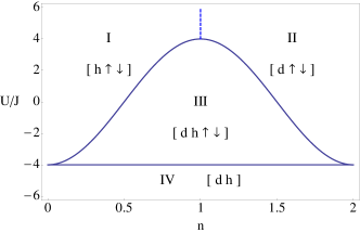
Figure 1: (Color online) Phase diagram of model (5) obtained for $\mathcal{J}_{0}(K)=0$ in $d=1$ aligia .

IV Away from the exact solution.

Deviation from the exactly solvable limit $X=1$ produces the new term

$$2\gamma\,J\sum_{\langle i,j\rangle,\sigma}[f^{\dagger}_{i\uparrow}f^{\dagger}_{j\downarrow}(e_{i}d_{j}+e_{j}d_{i})+\mathrm{h.c.}]\,,$$ (15)

where we have defined $\gamma\equiv\mathcal{J}_{0}(K)=1-X$. As these new terms allow doublons to convert into two single fermions on neighboring sites (and the reverse), the Hamiltonian no longer conserves the individual number of slave particles, and thus no exact solution is known. However, the $\eta$-symmetry is preserved and one expects that the enormous degeneracy of the ground state would again be removed. For $\gamma\simeq 1$, i.e. $|X|\ll 1$, the model can be treated using bosonization techniques and the phase diagram is known (also in the presence of nearest-neighbor interactions) japaridze showing for $U<0$ that superconducting correlations coexist with CDW. For the strongly-interacting case, exact diagonalization in 1D has been used arrachea ; nakamura , for systems of up to 12-14 sites. Nakamura nakamura presented a phase diagram at half and quarter filling (for $X=\pm 1/4$), and Arrachea et al. arrachea have shown that superconducting correlations can appear for $n=1$. However, the general picture for arbitrary filling is still missing.

In the next section we will use the QMC technique to investigate the charge and spin ordering of the Hamiltonian given by Eq. (5) at general values of $X$ and see how the results evolve between the two integrable cases ($X=0$ and $X=1$) for the specific case of half-filling.

V Quantum Monte Carlo method

To treat the Hamiltonian (5), we employed a standard “world-line” algorithm worldline . This is a finite-temperature method, operating in the canonical ensemble, which is particularly well-adapted to treat lattice spin-charge Hamiltonians. In order to sample the zero temperature behavior of the system, it is important to set the inverse temperature of the system, $\beta=1/kT$, to a sufficiently large value. By comparing the results for the ground state energy of the system with $\gamma=1$ to the exact results for the Hubbard model available from the Bethe Ansatz, we established that a sufficiently low temperature was $\beta J=48$, and accordingly we used this value in all the simulations. The Trotter decomposition of the imaginary time axis gives systematic errors which can be made arbitrarily small by increasing the number of timeslices, thereby reducing the imaginary-time discretization $\Delta\tau$. Our simulations demonstrated that the convergence of the results depended strongly on the value of $\gamma$. For the Hubbard model ($\gamma=1$) a relatively coarse value of $\Delta\tau=0.1$ was adequate. However, as $\gamma$ was reduced, $\Delta\tau$ also had to be reduced further, the lowest values of $\gamma=0.2$ requiring a discretization of $\Delta\tau\simeq 0.02$, with the simulation involving 2048 timeslices.

As well as the increased number of timeslices required, taking lower values of $\gamma$ was also hindered by ergodic “sticking”, in which local Monte Carlo (MC) updates are unable to evolve the system from local minima in energy. It was this factor that set the practical barrier on the lowest values of $\gamma$ that we were able to simulate, and accordingly we only present results for $\gamma\geq 0.2$. In order to obtain results of high accuracy, typically 16,000 MC measurements would be made for each set of parameters, with each measurement being separated by the next by several MC sweeps in order to reduce autocorrelation between the data.

A particular advantage of the world-line method is that as it operates in the real-space occupation number basis, it is simple to evaluate operators diagonal in number operators, such as the onsite spin $\sigma_{i}=n_{i\uparrow}-n_{i\downarrow}$, the onsite charge $\rho_{i}=n_{i\uparrow}+n_{i\downarrow}$, the doublon number, and correlations between these operators. An especially useful quantity is the static structure function

$$S_{\alpha}(q)=\frac{1}{L}\sum_{m,n}e^{iq\left(m-n\right)}\langle\alpha_{m}\alpha_{n}-\alpha^{2}\rangle$$ (16)

where $m$ and $n$ are integers labeling sites, $\alpha$ = $\sigma$ ($\rho$) denotes spin (charge), and $L$ is the number of lattice sites. As well as using the structure functions to investigate the type of spin and charge ordering present in the system, they can also be used to directly estimate the Luttinger-liquid parameters clay ,

$$K_{\alpha}=\mbox{lim}_{q\rightarrow 0}\frac{S_{\alpha}(q)}{\pi q}\,.$$ (17)

Thus, when the structure function is linear at low momentum, the Luttinger-liquid parameter is well-defined and is simply related to its slope. On the other hand, if the function is quadratic, this indicates that the Luttinger-liquid parameter is not well-defined and that this sector has a gap. In a uniform system, continuity requires that $S(q\rightarrow 0)=0$. However, if phase separation occurs $S(q)$ will have a peak at the smallest non-zero momentum, which will diverge as $L$ increases. The regularity of $S(q)$ for small momentum thus also provides a first check that the system is not phase-separated.

V.1 QMC results

Doublon density – In this section we will measure all energies in units of $J$. In Fig. 2 we show the doublon density as a function of $\gamma$ for several different values of the Hubbard interaction $U$. In these simulations, $\gamma$ was initially set to 1, and then reduced “quasi-statically” in steps of $\Delta\gamma=0.01$. For each value of $\gamma$ and $U$ the ensemble was allowed to rethermalize and a number (typically 64) of MC measurements made. This technique permits a rapid scan to be made through the configuration space of the model, at the expense of only producing results of moderate accuracy.

From Fig. 2, we can first see that for $U=0$, the doublon density does not depend on $\gamma$. This arises from the underlying symmetry of the Hamiltonian at half-filling. For negative $U$, we see that the doublon density increases as $\gamma$ is reduced, interpolating smoothly between the results for the Hubbard model ($\gamma=1$), and the exactly solvable case ($\gamma=0$). The results for positive $U$ mirror those for negative $U$, and can be related via

$$n_{d}(+|U|)=0.5-n_{d}(-|U|).$$ (18)

The validity of Eq. (18) is clear from the numerical results in Fig. 2. In addition, it can be easily proven, starting from Eq. (7) and recalling that $N_{d}=\sum_{i}n_{i\uparrow}n_{i\downarrow}$.

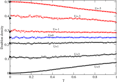
Figure 2: (Color online) Doublon density measured as $\gamma$ is quasi-statically reduced toward zero. For $U=0$ (blue squares) the doublon density does not change, reflecting the symmetry of the model. For positive $U$ (black circles) the density drops as $\gamma$ is reduced; the reverse is the case for negative $U$ (red squares). The data are symmetric about $n_{d}=0.25$ (see Eq. (18)). The solid lines are cubic fits to the data to guide the eye. The arrows on the left indicate the analytic values obtained in Ref. aligia for the limit $\gamma=0$. Parameters of the model: 32 sites, $\beta=48$, $n_{\uparrow}=n_{\downarrow}$.

Although $\gamma=0$ is not directly accessible to our QMC simulation due to ergodic trapping, we can obtain estimates for the doublon density in this limit by extrapolating the data in Fig. 2. We present the results in Fig. 3. The agreement between the numerical results and the exact solution aligia is excellent, demonstrating the accuracy and reliability of the QMC simulation.

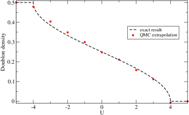
Figure 3: (Color online) Comparison of the analytic results for the doublon density for $\gamma=0$ with the results obtained by extrapolating the data shown in Fig. 2. The agreement is seen to be excellent.

Correlation functions – In Fig. 4a we show the static charge structure functions for strong repulsive interactions, $U=4$. It can be clearly seen that for the Hubbard model ($\gamma=1$) the charge sector is gapped, and that the structure function presents a weak peak at $k=2k_{F}=\pi$. Reducing $\gamma$ suppresses the structure function, and weakens this peak further. The spin structure function, shown in Fig. 4b shows a contrasting behavior. For the Hubbard model this function possesses a strong peak at $2k_{F}$, indicating the presence of strong antiferromagnetic ordering $(\uparrow,\downarrow,\uparrow,\downarrow)$, and this peak is enhanced as $\gamma$ is reduced. An infinitesimally small deviation of the coupling $\gamma$ from zero opens channels for the exchange of spins on neighboring sites. This gives a preference for an alternating distribution of particles with opposite spins along the lattice, i.e. a spin-density-wave (SDW) structure. The spin excitations are gapless, and the spin-$SU(2)$ symmetry sets the Luttinger-liquid parameter $K_{\sigma}=1$.

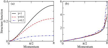
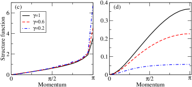
Figure 4: (Color online) (a) Charge structure function for the half-filled model with $U=4$. For $\gamma=1$ there is a weak peak at $k=\pi$; as $\gamma$ is reduced this peak is suppressed. (b) Spin structure function. For $\gamma=1$ there is a strong peak at $k=\pi$ indicating strong antiferromagnetic ordering. This peak is enhanced as $\gamma$ is reduced. (c) As above, but for $U=-4$. (d) As above, but for $U=-4$. The effect of changing the sign of $U$ is to interchange the spin and charge degrees of freedom. Momentum is measured in units of the inverse lattice spacing.

Below these plots we show the corresponding structure functions for attractive interaction $U=-4$. It can be clearly seen that changing the sign of $U$ simply has the effect of interchanging the spin and charge degrees of freedom, as noted in Section II. In this case we see that reducing $\gamma$ now has the effect of suppressing the spin dynamics, while enhancing the staggered charge order $(d,h,d,h)$. Similarly to before, deviation from the exact solution for $\gamma=0$ opens channels for an alternating distribution of doublons and holons along the lattice i.e. a charge-density-wave (CDW) structure. Now the spin degrees of freedom are gapped, the charge excitations are gapless, and due to the charge-$SU(2)$ symmetry, the Luttinger-liquid parameter $K_{\rho}=1$.

Results for $U=-2$ are given in Fig. 5. Looking first at the charge structure function, the result for the Hubbard model looks similar to that seen previously for $U=-4$. As $\gamma$ is reduced, however, a new behavior emerges. When $\gamma$ is reduced below 0.6, the charge structure function forms a peak at an incommensurate momentum, indicating the formation of an incommensurate CDW. At the same time an incommensurate SDW forms in the spin sector, at a smaller value of momentum. This incommensurate ordering is reminiscent of the behavior known for stripes in the 2D conventional Hubbard model upon doping zaanen .

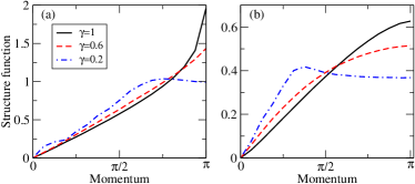
Figure 5: (Color online) (a) Charge structure function for $U=-2$. As $\gamma$ is reduced below 0.6, the system forms an incommensurate CDW. (b) Spin structure function for $U=-2$. For low $\gamma$ the system also forms an incommensurate SDW. Momentum is measured in units of the inverse lattice spacing.

The incommensurate order occurs generally for low values of $\gamma$ for $|U|<4$ (region III of the phase diagram Fig. 1). Reducing $|U|$ further to $U=0$ shows the effect of $\gamma$ on a non-interacting system. For $\gamma=1$ the system consists of free fermions, and as can be seen in Fig. 6 the charge and spin correlators are identical to each other and are featureless. At $\gamma=0.6$ the dynamics of the system is again slightly suppressed, but at a $\gamma=0.2$ the system again manifests incommensurate charge and spin order, with the structure functions peaking at $k=k_{F}$.

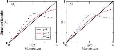
Figure 6: (Color online) (a) Charge structure function for $U=0$. (b) Spin structure function for $U=0$. For the non-interacting case the charge and spin degrees of freedom behave identically. At $\gamma=1$ they show no structure (free fermions), but form incommensurate ordered phases for low $\gamma$. Momentum is measured in units of the inverse lattice spacing.

Let us try to understand how these results connect to the exact solution for $|U|\leq 4$. In this case the ground state consists of a finite number of doublons and holons, separated by singly occupied sites to ensure their maximal delocalization along the lattice. Thus, in this sector a rather special ordering, characterized by coexistence of CDW and SDW order on different lattice sites, is possible. For a more detailed description let us consider few particular cases.

Let us start from the $U=0$ case, where $n_{d}=0.25$. The ground state configuration at $X\simeq 1$ consists of an alternating distribution of doublons and holons, separated by single occupied sites with alternating spins on these sites. A possible configuration would be

$$(\,d\,\uparrow\,h\,\downarrow\,d\,\uparrow\,h\,\downarrow\,d\,\uparrow\,h\,\downarrow\,...)$$

showing the coexistence of period-4 charge and spin density modulations, as observed in Fig. 6.

At $U=-2$, where $n_{d}=0.3(3)$, a possible configuration would be

$$(\,d\,\uparrow\,h\,d\,\downarrow\,h\,d\,\uparrow\,h\,d\,\downarrow\,h\,\,\,...)$$

showing the coexistence of a period-3 charge modulation with a period-6 spin density modulation.

For other values of $U$, the number of doublons (and singly occupied sites) will be in general incommensurate. The structure of the coexisting charge and spin density waves must reflect this incommensurability, and will consequently be much more complicated.

For $0<U<4$, the behavior is the same as for $-4<U<0$, but with the spin and charge structure functions inverted. For instance, for $U=2$ Fig. 5a would hold for spin and Fig. 5b would hold for charge, indicating an incommensurate spin-charge-density wave.

To ensure that the behavior we have seen is not an artifact of the finite system size, we have repeated our simulations for $U=2.5$ for lattice sizes between 16 sites and 100 sites. We show the results in Fig. 7, and it is clear that the incommensurate structure seen in the structure functions hardly alters as the lattice size is increased. We can thus be confident that our standard size of $L=32$ is sufficiently large for finite size effects to be neglected.

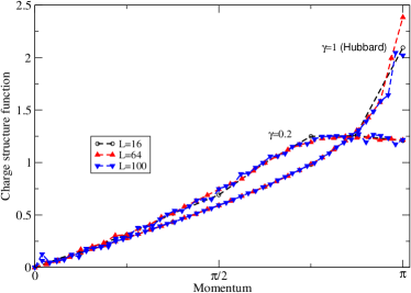
Figure 7: (Color online) The charge structure function for $U=-2.5$ as the lattice size is increased. The results show little dependence on lattice size, indicating that finite size effects are not important in our analysis. Momentum is measured in units of the inverse lattice spacing.

From the simulation we have also evaluated the Luttinger parameter $K_{\rho}$, using Eq. (17). As shown in Fig. 8, for $\gamma=1$ $K_{\rho}$ is equal to 1 for negative values of $U$ (the 10% deviation is within the numerical error of our calculation), indicating the coexistence of superconductivity and charge wave ordering. As $U$ becomes positive, a gap opens in the charge sector and $K_{\rho}$ can no longer strictly be defined for the half-filled case. This is marked in Fig. 8 by the calculated value of this parameter abruptly dropping, as the charge structure function is no longer linear at small momentum. For $\gamma=0.6$ a similar behavior is seen, except that the opening of the charge gap now occurs at a higher value of $U\simeq 1.8$. As $\gamma$ is reduced further this trend continues, and for $\gamma=0.2$ we find that the critical $U$ has a value of approximately 3.5, in good agreement with the estimate given in Ref. aligia .

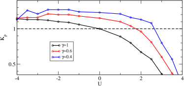
Figure 8: (Color online) Luttinger-liquid parameter $K_{\rho}$. For $\gamma=1$, $K_{\rho}$ is approximately equal to 1 for negative $U$, then drops as $U$ becomes positive, signaling the opening of the charge gap. As $\gamma$ is decreased, this drop occurs at larger values of $U$. The dashed line is a guide to the eye, to assist in estimating where the drop occurs.

Before closing this section, we want to mention that a model, similar to the one presented here, but without the three-body term, has been been previously investigated anfossi ; montorsi . For this so-called Hirsch model (see for instance Ref. hirsch2 ), the strongly-correlated regime at half-filling exhibits an incommensurate (singlet) superconducting phase that show many similarities with our findings. This phase has been captured using density-matrix renormalization group techniques (DMRG), while bosonization and RG were unable to describe the transition dobry .

At present, the phase diagram of the model (5) in 1D is only partially known; however, as we will show in the last section, the model can describe realistic experiments using cold atoms. This represents a good challenge for quantum simulations, as well as for new numerical calculations. A fascinating possibility would be an emerging superconducting phase, with tightly bound pairs of momentum $\pi$.

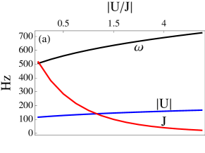
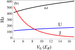
Figure 9: (Color online) Comparison between frequency modulation $\omega$ of the magnetic field, hopping parameter $J$ and Hubbard interaction $U$ (all measured in Hz) at the zero of the Bessel function $\mathcal{J}_{0}(U_{1}/\hbar\omega)$ for ${}^{40}K$ close to a zero of a Feshbach resonance ($B_{0}(G)=224.2$, $\Delta(G)=9.7$ and $a_{bg}/a_{0}=174$). (a) In the attractive case $a_{0}<0$, we have chosen $B_{m}(G)=233.5$ and $B_{1}(G)=4$; (b) in the repulsive case $a_{0}>0$, we have chosen $B_{m}(G)=234.36$ and $B_{1}(G)=4$. The optical lattices parameters are $V_{x}=V_{y}=25\,E_{R}$, $V_{z}=V_{0}$ and $\lambda=1064\mathrm{nm}$.

VI Experimental parameters.

For the experimental realization of this model (in 1D for instance) we consider an optical lattice $V(\textbf{r})=V_{x}\sin^{2}(kx)+V_{y}\sin^{2}(ky)+V_{z}\sin^{2}(kz)$ with $k=2\pi/\lambda$ generated by a laser with wavelength $\lambda=1064\mathrm{nm}$; we take the limit $V_{x},\,V_{y}\gg V_{z}$ to allow dynamics only in one dimension. We studied the Feshbach resonance for ${}^{40}K$ at $B_{0}(G)=224.2$, characterized by a width $\Delta(G)=9.7$ and a background scattering length $a_{bg}/a_{B}=174$, where $a_{B}$ denotes the Bohr radius grimm . The dependence of the scattering length $a_{s}$ on the magnetic field $B$ is given near resonance by

$$a_{s}=a_{bg}\left(1-\frac{\Delta}{B-B_{0}}\right)\,.$$ (19)

We choose a time dependent magnetic field of the form $B(t)=B_{m}+B_{1}\cos(\omega t)$ and consider $|B_{1}|\ll|B_{m}-B_{0}|$. Therefore, at first order in $B_{1}/(B_{m}-B_{0})$ we can write

$$a_{s} \simeq a_{bg}\left[1-\frac{\Delta}{B_{m}-B_{0}}\left(1-\frac{B_{1}\cos(\omega t)}{B_{m}-B_{0}}\right)\right]$$ (20)

$$\equiv a_{0}+a_{1}\cos(\omega t)\,,$$

where we have defined $a_{0}=a_{bg}[1-\Delta/(B_{m}-B_{0})]$ and $a_{1}=-a_{bg}B_{1}\Delta/(B_{m}-B_{0})^{2}$.

In Figs. 9(a) and (b), we plot the driving frequency values corresponding to the zero of the Bessel function $\mathcal{J}_{0}(U_{1}/\hbar\omega)=0$ both in the attractive and repulsive case, respectively, in a particular range of parameters near the zero of the Feshbach resonance (so that we can reach the region of interest in the regime of strong coupling analyzed in this paper) and compare with an estimate of $U$ and $J$ for the 1D case. We find that $\omega$ is in the sub-kilohertz regime $\omega\simeq 2\pi\times 500-600\mathrm{Hz}$ and we observe that such a choice of parameters fulfills the main approximations required from Floquet theory, i.e. $\omega\gg U,\,J$. Actually, in typical experiments lignier2007 the kilohertz energy scale is far below the band gap and higher band contributions do not play a role, except for possible multiphoton processes. Moreover, one can see that the range where Floquet theory can be applied for this choice of parameters of the resonance allows us to explore the phase diagram in the main region of interest, where the correlated-hopping model should reveal interesting phenomena. Such a choice of parameters plotted in Fig. 9 can be considered as an example to show that the model described here can be realized in experiments; one would envisage that for different values or ranges of $U/J$, the optimal parameters will be chosen accordingly. We finally want to mention that to calculate the parameters $U$ and $J$ we have used the approximate formulas (given in terms of the recoil energy $E_{R}=\hbar^{2}(2\pi/\lambda)^{2}/2m$, with $m$ denoting the atomic mass) bloch1 : $U/E_{R}=(2\pi/\lambda)a_{s}\sqrt{8/\pi}\,V_{0}^{1/4}\,V_{x,y}^{1/2}$ and $J/E_{R}=(4/\sqrt{\pi})\,V_{0}^{3/4}e^{-2\sqrt{V_{0}}}$, where we have introduced the potential depth $V_{0}=V_{z}$ (assuming that the electron dynamics would be in the $z$ direction), and frozen the motion in the $x$ and $y$ directions taking $V_{x}=V_{y}=25\,E_{R}$ such that we can consider one-dimensional effective systems.

VII Conclusions.

We have discussed a scheme for cold atoms to engineer an extension of the Hubbard model that includes nearest-neighbor correlations affecting the hopping processes for fermions in optical lattices. After imposing a time-dependent driving of the $s$-wave scattering length between atoms in two different hyperfine states (that we have modeled as a pseudo-spin $1/2$ system assuming no spin imbalance), we have shown within Floquet theory that the system can be described by an effective Hamiltonian with correlated-hopping interactions. The model has an additional SU(2) symmetry, with respect to the usual spin-SU(2) symmetry of the Hubbard model, generated by the algebra of $\eta$ operators. This fact opens the possibility of searching for a ground state characterized by the exotic $\eta$-pairing superconductivity proposed by Yang in 1989 as a metastable state of the Hubbard model. This model, for the particular case of $d=1$ on which we focused in this work, has two integrable points as a function of the driving parameter $X$ that tunes the coupling of the correlated-hopping interactions: one is the Hubbard model ($X=0$) and the other one ($X=1$) has been analyzed in Ref. aligia by Arrachea and Aligia. The integrable point discussed by them manifests $\eta$-pairing in the ground state. Unfortunately, the huge degeneracy of the ground state prevents the system from showing superconducting properties, like anomalous flux quantization aligiaflux . Exploring this region of the phase diagram that extends over the whole filling axis (see Fig. 1, region III) can be quite challenging in general for experiments. Indeed, as discussed for the case of the supersymmetric model by Essler et al. essler , it is possible to draw the phase diagram of Fig. 1 using the grand canonical ensemble. Such representation is of fundamental importance because in typical cold atom systems the presence of the trap can be interpreted, in the local density approximation (LDA), as a local chemical potential such that different shells with different quantum phases would appear radially in the trapped gas. The consequence of this, however, is that the central “dome” (region III) would correspond to a single value of chemical potential $\mu=0$, thus rendering its observation problematic.

We have focused on the study of the half-filled model, away from the integrable point $X=1$, using the “world-line” algorithm to perform QMC simulations . We have explored the parameter space in the strong coupling regime, where known analytical methods like bosonization and RG techniques cannot be employed. We have found that an incommensurate order in the charge and the spin sector sets in for the ratio $|U/J|<4$, where $U$ and $J$ are respectively the on-site interaction and the bare hopping amplitude. We have observed that the two kinds of orders manifests as a peak in the spin and charge structure functions at incommensurate (distinct) momenta. The two orders exchange their behavior when $U\rightarrow-U$ as expected from the symmetries of the model. In particular, for the case $U=0$ a peak appears exactly at $k_{F}=\pi/2$ in both structure functions.

A further investigation of the model would require the measurement of other types of orders, to see, for instance, what role is played by superconductivity when the incommensurate spin and charge order appears. These types of correlations cannot be computed with the QMC algorithm used in this work since it is based on a number-conserving representation of the fermionic Hilbert space; one would thus need to employ other techniques to look, for instance, at the 2-body density matrix. Moreover, deviations from half-filling are still to be studied in the strong coupling regime and the phase diagram has not been established yet, except for the case $X=1/4$ nakamura .

In dimensions $d\geq 2$, the physics of the model is almost all to be explored; weak-coupling Hartree-Fock calculations in $d=2$ show that the model can exhibit $d$-wave superconductivity arracheadwave . A very interesting possibility, deferred to further studies, would be the appearance of $\eta$-superconductivity in the ground state.

VIII Acknowledgments.

We are thankful to L. Santos for pointing out the problem concerning the observation of phase III in trapped systems. We also acknowledge A. Montorsi, M. Roncaglia, P. Barmettler, M. Dalmonte, and A. Hemmerich for useful discussions, and F. Sols for insight regarding ODLRO. This work was supported by the Netherlands Organization for Scientific Research (NWO) and by the Spanish MICINN through Grant No. FIS-2010-21372 (CEC).

*

Appendix A Derivation of the effective model

The Hamiltonian of the Hubbard model with a time-dependent interaction reads:

$$H = -J\sum_{\langle i,j\rangle,\sigma}(c^{\dagger}_{i\sigma}c_{j\sigma}+\mathrm{h.c.})+\bar{U}(t)\sum_{i}n_{i\uparrow}n_{i\downarrow}$$ (21)

$$= -J\sum_{\langle i,j\rangle,\sigma}(c^{\dagger}_{i\sigma}c_{j\sigma}+\mathrm{h.c.})+U\sum_{i}n_{i\uparrow}n_{i\downarrow}+U_{1}\cos(\omega t)\sum_{i}n_{i\uparrow}n_{i\downarrow}$$

$$\equiv H_{J}+H_{U}+H_{\mathrm{d}}(t)\,.$$

Let us define the following Floquet basis

$$|\left\{n_{j\sigma}\right\},m\rangle=|\left\{n_{j\sigma}\right\}\rangle\exp\left(-i\frac{U_{1}}{\hbar\omega}\sin(\omega t)\sum_{j}n_{j\uparrow}n_{j\downarrow}+im\omega t\right)\,,$$ (22)

where $|\left\{n_{j\sigma}\right\}\rangle$ stands for a Fock state, and compute the Floquet Hamiltonian matrix elements using this basis (the double brackets indicates the time average)

$$\langle\langle\left\{n^{\prime}_{j\sigma}\right\},m^{\prime}|H-i\hbar\partial_{t}|\left\{n_{j\sigma}\right\},m\rangle\rangle\,.$$ (23)

The derivative $-i\hbar\partial_{t}|\left\{n_{j\sigma}\right\},m\rangle$ cancels with $H_{\mathrm{d}}(t)|\left\{n_{j\sigma}\right\},m\rangle$. Let us examine $H_{U}$: we have to calculate the following term

$$\frac{1}{T}\int_{0}^{T}\,dt\,e^{i\omega t(m-m^{\prime})}\langle\left\{n^{\prime}_{j\sigma}\right\}|H_{U}|\left\{n_{j\sigma}\right\}\rangle\exp\left[-i\frac{U_{1}}{\hbar\omega}\sin(\omega t)\sum_{j}(n_{j\uparrow}n_{j\downarrow}-n^{\prime}_{j\uparrow}n^{\prime}_{j\downarrow})\right]\,.$$ (24)

$|\left\{n_{j\sigma}\right\}\rangle$ are eigenstates of $H_{U}$, hence $n_{j\sigma}=n^{\prime}_{j\sigma},\,\,\forall j$ and we find

$$\frac{1}{T}\int_{0}^{T}\,dt\,e^{i\omega t(m-m^{\prime})}\langle\left\{n^{\prime}_{j\sigma}\right\}|H_{U}|\left\{n_{j\sigma}\right\}\rangle=\langle\left\{n^{\prime}_{j\sigma}\right\}|H_{U}|\left\{n_{j\sigma}\right\}\rangle\delta_{m,m^{\prime}}\,.$$ (25)

For the hopping part, we have to calculate

$$\frac{1}{T}\int_{0}^{T}dt\,e^{i\omega t(m-m^{\prime})}\langle\left\{n^{\prime}_{j\sigma}\right\}|H_{J}|\left\{n_{j\sigma}\right\}\rangle\exp\left[-i\frac{U_{1}}{\hbar\omega}\sin(\omega t)\sum_{j}(n_{j\uparrow}n_{j\downarrow}-n^{\prime}_{j\uparrow}n^{\prime}_{j\downarrow})\right]\,.$$ (26)

It is crucial now to evaluate the term $\langle\left\{n^{\prime}_{j\sigma}\right\}|H_{J}|\left\{n_{j\sigma}\right\}\rangle$. The typical form of this quantity is

$$\langle\left\{n^{\prime}_{j\sigma}\right\}|c^{\dagger}_{i\sigma}c_{k\sigma}|\left\{n_{j\sigma}\right\}\rangle\,.$$ (27)

If $\sigma=\,\uparrow$ (and then define $\bar{\sigma}\equiv\,\downarrow$), it implies that $n^{\prime}_{i\sigma}=n_{i\sigma}+1$, $n^{\prime}_{i\bar{\sigma}}=n_{i\bar{\sigma}}$, $n^{\prime}_{k\sigma}=n_{k\sigma}-1$, $n^{\prime}_{k\bar{\sigma}}=n_{k\bar{\sigma}}$ and $n^{\prime}_{j\rho}=n_{j\rho}$ for $j\neq i,\,k$. As a consequence, the density dependent part in the exponential becomes

$$\hat{s}\equiv\sum_{j}(n_{j\uparrow}n_{j\downarrow}-n^{\prime}_{j\uparrow}n^{\prime}_{j\downarrow})=n_{i\uparrow}n_{i\downarrow}+n_{k\uparrow}n_{k\downarrow}-(n_{i\uparrow}+1)n_{i\downarrow}-(n_{k\uparrow}-1)n_{k\downarrow}=-n_{i\downarrow}+n_{k\downarrow}\,.$$ (28)

An analogous result holds for $\sigma=\,\downarrow$. We now use the integral representation of Bessel functions of first kind:

$$\mathcal{J}_{n}(x)=\frac{1}{2\pi}\int_{-\pi}^{\pi}\,dt\,e^{i(x\sin t-nt)}\,,$$ (29)

define $\tau=\omega t$ and then shift $\tau\rightarrow\tau+\pi$. The integral then becomes

$$\frac{1}{2\pi}\int_{-\pi}^{\pi}\,d\tau\,e^{i(\tau+\pi)(m-m^{\prime})-i\frac{U_{1}}{\hbar\omega}\hat{s}\sin(\tau+\pi)}=\frac{(-1)^{m-m^{\prime}}}{2\pi}\int_{-\pi}^{\pi}\,d\tau\,e^{i\tau(m-m^{\prime})+i\frac{U_{1}}{\hbar\omega}\hat{s}\sin\tau}\,,$$ (30)

which yields

$$(-1)^{m-m^{\prime}}\mathcal{J}_{m^{\prime}-m}\left(\frac{U_{1}}{\hbar\omega}\hat{s}\right)\,,$$ (31)

that can be reabsorbed in $H_{J}$. In the large frequency limit $\hbar\omega\gg J,U$, the off-diagonal elements of the Floquet Hamiltonian can be (perturbatively) neglected and we can thus consider only $m=m^{\prime}$ and choose $m=0$ in the first Floquet Brillouin zone. Therefore, the approximate form of the Floquet Hamiltonian is

$$H_{\mathrm{eff}}=-J\sum_{\langle i,j\rangle,\sigma}(c^{\dagger}_{i\sigma}c_{j\sigma}+\mathrm{h.c.})\mathcal{J}_{0}\left[K(n_{i\bar{\sigma}}-n_{j\bar{\sigma}})\right]+U\sum_{i}n_{i\uparrow}n_{i\downarrow}\,.$$ (32)

where we defined $K\equiv U_{1}/\hbar\omega$.

References

- (1) D. Jaksch, C. Bruder, J. I. Cirac, C. W. Gardiner, and P. Zoller, Phys. Rev. Lett. 81, 3108 (1998).
- (2) M. Greiner, O. Mandel, T. Esslinger, T. W. Hänsch, and I. Bloch, Nature 415, 39 (2002).
- (3) W. Hofstetter, J. I. Cirac, P. Zoller, E. Demler, and M. D. Lukin, Phys. Rev. Lett. 89, 220407 (2002).
- (4) R. Jördens, N. Strohmaier, K. Günter, H. Moritz, and T. Esslinger, Nature 455, 204 (2008).
- (5) J. Dalibard, F. Gerbier, G. Juzeliunas, and P. Öhberg, Rev. Mod. Phys. 83, 1523 (2011).
- (6) L.-K. Lim, C. Morais Smith, and A. Hemmerich, Phys. Rev. Lett. 100, 130402 (2008).
- (7) M. Aidelsburger, M. Atala, M. Lohse, J. T. Barreiro, B. Paredes, and I. Bloch, Phys. Rev. Lett 111, 185301 (2013).
- (8) H. Miyake, G. A. Siviloglou, C. J. Kennedy, W. C. Burton, and W. Ketterle, Phys. Rev. Lett. 111, 185302 (2013).
- (9) N. Goldman, W. Beugeling, and C. Morais Smith, Europhys. Lett.) 97, 23003 (2012).
- (10) M. Lewenstein, A. Sanpera, V. Ahufinger, B. Damski, A. Sen, and U. Sen, Advances in Physics 56, 243 (2007).
- (11) I. Bloch, J. Dalibard, and W. Zwerger, Rev. Mod. Phys. 80, 885 (2008).
- (12) I. Bloch, J. Dalibard, and S. Nascimbène, Nature Physics 8, 267 (2012).
- (13) D. Greif, T. Uehlinger, G. Jotzu, L. Tarruell, and T. Esslinger, Science 340, 1307 (2013).
- (14) André Eckardt, Christoph Weiss, and Martin Holthaus, Phys. Rev. Lett. 95, 260404 (2005).
- (15) C. E. Creffield and T. S. Monteiro, Phys. Rev. Lett. 96, 210403 (2006).
- (16) H. Lignier, C. Sias, D. Ciampini, Y. Singh, A. Zenesini, O. Morsch, and E. Arimondo, Phys. Rev. Lett. 99, 220403 (2007).
- (17) A. Eckardt, P. Hauke, P. Soltan-Panahi, C. Becker, K. Sengstock, and M. Lewenstein, EPL (Europhysics Letters) 89, 10010 (2010).
- (18) J. Struck, C. Ölschläger, R. Le Targat, P. Soltan-Panahi, A. Eckardt, M. Lewenstein, P. Windpassinger, and K. Sengstock, Science 333, 996 (2011).
- (19) J. Struck, C. Ölschläger, M. Weinberg, P. Hauke, J. Simonet, A. Eckardt, M. Lewenstein, K. Sengstock, and P. Windpassinger, Phys. Rev. Lett. 108, 225304 (2012).
- (20) P. Hauke, O. Tieleman, A. Celi, C. Ölschläger, J. Simonet, J. Struck, M. Weinberg, P. Windpassinger, K. Sengstock, M. Lewenstein, and A. Eckardt, Phys. Rev. Lett. 109, 145301 (2012).
- (21) Á. Rapp, X. Deng, and L. Santos, Phys. Rev. Lett. 109, 203005 (2012).
- (22) M.E. Foglio and L.M. Falicov, Phys. Rev. B 20, 4554 (1979).
- (23) M. Grifoni and P. Hänggi, Phys. Rep. 304, 229 (1998).
- (24) H. Sambe, Phys. Rev. A 7, 2203 (1973).
- (25) J. Hubbard, Proc. Roy. So. London A 276, 238 (1963).
- (26) L. M. Duan, EPL (Europhysics Letters) 81, 20001 (2008).
- (27) J. P. Kestner, Phys. Rev. A 81, 043618 (2010).
- (28) L. Arrachea and A. A. Aligia, Phys. Rev. Lett. 73, 2240 (1994).
- (29) C. N. Yang, Phys. Rev. Lett. 63, 2144 (1989).
- (30) C. N. Yang, Rev. Mod. Phys. 34, 694 (1962).
- (31) G.L. Sewell, J. Stat. Phys. 61, 415 (1995).
- (32) H. T. Nieh, G. Su, and B. H. Zhao, Phys. Rev. B 51, 3760 (1995).
- (33) R. R. P. Singh, and R. T. Scalettar, Phys. Rev. Lett. 66, 3203 (1991).
- (34) F. H. L. Essler, V. E. Korepin, and K. Schoutens, Phys. Rev. Lett. 68, 2960 (1992).
- (35) F. H. L. Essler, V. E. Korepin, and K. Schoutens, Phys. Rev. Lett. 70, 73 (1993).
- (36) J. de Boer, V. E. Korepin, and A. Schadschneider, Phys. Rev. Lett. 74, 789 (1995).
- (37) J. de Boer, and A. Schadschneider, Phys. Rev. Lett. 75, 4298 (1995).
- (38) A. Schadschneider, Phys. Rev. B 51, 10386 (1995).
- (39) L. Arrachea, A. A. Aligia, and E. Gagliano, Phys. Rev. Lett. 76, 4396 (1996).
- (40) G. I. Japaridze and A. P. Kampf, Phys. Rev. B 59, 12822 (1999).
- (41) A. A. Aligia and L. Arrachea, Phys. Rev. B 60, 15332 (1999).
- (42) H. Frahm and V.E. Korepin, Phys. Rev. B 42, 10553 (1990).
- (43) L. Arrachea, A. A. Aligia, E. Gagliano, K. Hallberg, and C. Balseiro, Phys. Rev. B 50, 16044 (1994).
- (44) M. Nakamura, Phys. Rev. B 61, 16377 (2000).
- (45) J.E. Hirsch, R.L. Sugar, D.J. Scalapino and R. Blankenbecler, Phys. Rev. B 26, 5033 (1982).
- (46) R. T. Clay, A. W. Sandvik, and D. K. Campbell, Phys. Rev. B 59, 4665 (1999).
- (47) J. Zaanen and O. Gunnarsson, Phys. Rev. B 40, 7391 (1989).
- (48) A. Anfossi, C. Degli Esposti Boschi, A. Montorsi, and F. Ortolani, Phys. Rev. B 73, 085113 (2006).
- (49) A. A. Aligia, A. Anfossi, L. Arrachea, C. Degli Esposti Boschi, A. O. Dobry, C. Gazza, A. Montorsi, F. Ortolani, and M. E. Torio, Phys. Rev. Lett. 99, 206401 (2007).
- (50) J. E. Hirsch, and F. Marsiglio, Phys. Rev. B 39, 11515 (1989).
- (51) A. O. Dobry and A. A. Aligia, Nucl. Phys. B 843, 767 (2011).
- (52) C. Ching, R. Grimm, P. Julienne, and E. Tiesinga, Rev. Mod. Phys. 82, 1225 (2010).
- (53) L. Arrachea and A. A. Aligia, Phys. Rev. B 59, 1333 (1999).
*