Abstract

One outcome of interspecific hybridization and subsequent effects of evolutionary forces is introgression, which is the integration of genetic material from one species into the genome of an individual in another species. The evolution of several groups of eukaryotic species has involved hybridization, and cases of adaptation through introgression have been already established. In this work, we report on a new comparative genomic framework for detecting introgression in genomes, called PhyloNet-HMM, which combines phylogenetic networks, that capture reticulate evolutionary relationships among genomes, with hidden Markov models (HMMs), that capture dependencies within genomes. A novel aspect of our work is that it also accounts for incomplete lineage sorting and dependence across loci. Application of our model to variation data from chromosome 7 in the mouse (Mus musculus domesticus) genome detects a recently reported adaptive introgression event involving the rodent poison resistance gene Vkorc1, in addition to other newly detected introgression regions. Based on our analysis, it is estimated that about 12% of all sites within chromosome 7 are of introgressive origin (these cover about 18 Mbp of chromosome 7, and over 300 genes). Further, our model detects no introgression in two negative control data sets. Our work provides a powerful framework for systematic analysis of introgression while simultaneously accounting for dependence across sites, point mutations, recombination, and ancestral polymorphism.

Author Summary

Hybridization is the mating between individuals from two different species. While hybridization introduces genetic material into a host genome, this genetic material may be transient and is purged from the population within a few generations after hybridization. However, in other cases, the introduced genetic material persists in the population—a process known as introgression—and can have significant evolutionary implications. In this paper, we introduce a novel method for detecting introgression in genomes using a comparative genomic approach. The method scans multiple aligned genomes for signatures of introgression by incorporating phylogenetic networks and hidden Markov models. The method allows for teasing apart true signatures of introgression from spurious ones that arise due to population effects and resemble those of introgression. Using the new method, we analyzed three sets of variation data from chromosome 7 in mouse genomes. The method detected previously reported introgressed regions as well as new ones in one of the data sets. In the other two data sets, which were selected as negative controls, the method detected no introgression. Our method enables systematic comparative analyses of genomes where introgression is suspected, and can work with genome-wide data.

Introduction

Hybridization is the mating between species that can result in the transient or permanent transfer of genetic variants from one species to another. The latter outcome is referred to as introgression. Mallet [1] recently estimated that “at least 25% of plant species and 10% of animal species, mostly the youngest species, are involved in hybridization and potential introgression with other species.” Introgression can be neutral and go unnoticed in terms of phenotypes but can also be adaptive and affect phenotypes. Recent examples of adaptation through hybridization include resistance to rodenticides in mice [2] and mimicry in butterflies [3]. Detecting regions with signatures of introgression in eukaryotic genomes is of great interest, given the consequences of introgression in evolutionary biology, speciation, biodiversity, and conservation [1]. With the increasing availability of genomic data, it is imperative to develop techniques that detect genomic regions of introgressive descent.

Let us consider an evolutionary scenario where two speciation events result in three extant species A, B, and C, with A and B sharing a most recent common ancestor. Further, some time after the splitting of A and B, hybridization occurs between B and C (that is, sexual reproduction of individuals from these two species). This scenario is depicted by the phylogenetic network in Fig. 1.

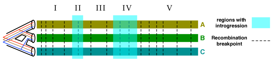
Figure 1: Evolutionary and genomic views of three genomes involving introgression. Hybridization between species B and C results in individuals of species B with genomes that are mosaics with regions of “vertical” descent from B and others of introgressive descent from C. Walking along the genomes from left to right, local gene genealogies are observed, and when a recombination breakpoint is crossed, the local genealogy changes. Switching of local gene genealogies of unlinked (broken by recombination) loci is known as incomplete lineage sorting (ILS). Further, the walk enters regions of introgressive descent (II and IV), where the genealogies switch due to hybridization. The complexity of the model stems from the co-occurrence of ILS and introgression, and the need to tease them apart. Within the phylogenetic network of the species (leftmost), three possible gene genealogies are shown: one that agrees with how species split and diverged (red), one that is reflective of the introgression event (blue), and another that is a signature of ILS (brown).

Immediately upon hybridization, approximately half of the hybrid individual’s genome comes from an individual in species $B$, whereas the remainder comes from an individual in species $C$. However, in homoploid hybridization, where the hybrid offspring has the same ploidy level as the two parental species, hybridization is often followed by back-crossing (further mating between the hybrid population and either of the two parental populations). Repeated back-crossing, followed by the effects of genetic drift and natural selection, results in genomes in the hybrid individuals that are mosaics of genomic material from the two parental species, yet not necessarily with a 50-50 composition. Thus, detecting introgressed regions requires scanning across the genome and looking for signals of introgression.

In a comparative framework, detecting introgressed regions can be achieved by evolutionary analysis of genomes from the parental species, as well as genomes from introgressed individuals. In such an analysis, a walk across the genomes is taken, and local phylogenies are (or, genealogies) are inspected; incongruence between two local phylogenies can be taken as a signal of introgresison [4]. However, in reality, the analysis is more involved than this, owing to potentially confounding signal produced by several factors, major of which is incomplete lineage sorting (ILS). As recombination breaks linkage across loci in the genome, the result is independent loci that may have different genealogies by chance, which is known as ILS. ILS is common to several groups of eukaryotic taxa where species diverged recently and not enough time has elapsed for all genomic loci to completely sort, resulting in a scenario where introgression and ILS effects need to be distinguished [5, 6, 7, 3, 8]. Fig. 1 illustrates this issue, where local genealogies across recombination breakpoints differ due to ILS, but also differ inside vs. outside introgressed regions. While other factors, such as gene duplication and loss [9], could potentially add to the complexity of the phylogenetic and genomic patterns, we focus here on introgression and ILS.

Recently, new methods were proposed to detect introgression in the presence of ILS. Durand et al.’s $D$ statistic allows for a sliding-window analysis of three-taxon data sets, while accounting for introgression and ancestral polymorphism [10]. However, this statistic assumes an infinite-sites model and independence across loci. Yu et al. [11] proposed a new statistical model for the likelihood of a species phylogeny model, given a set of gene genealogies, accounting for both ILS and introgression. However, this model does not work directly from the sequences; rather, it assumes that gene genealogies have been estimated, and computations are based on these estimates. Further, the model assumes independence across loci. Of great relevance to our work here is a group of hidden Markov model (HMM) based techniques were introduced recently for analyzing genomic data in the presence of recombination and ILS [12, 13, 14]; however, these methods do not account for introgression. A recent extension [15] was devised to investigate the effects of population structure.

In this paper, we devise a novel model based on integrating phylogenetic networks with hidden Markov models (HMMs). The phylogenetic network component of our model captures the relatedness across genomes (including point mutation, recombination, ILS, and introgression), and the HMM component captures dependence across sites and loci within each genome. Using dynamic programming algorithms [16] paired with a multivariate optimization heuristic [17], the model can be trained on genomic data, and allows for the identification of genomic regions of introgressive descent. We applied our model to chromosome 7 genomic variation data from three mouse data sets. Our analysis recovered an introgression event involving the rodenticide resistance gene VKORC1, which was recently reported in the literature [2]. Further, our analysis indicates that about 12% of sites within chromosome 7 are in fact of introgressive origin, which is a novel finding. Further, when applied to two negative control data sets, our model did not detect any introgression, further attesting to its robustness. Our model will enable new analyses of eukaryotic data sets where introgression is suspected, and will further help shed light on the Tree of Life—or, Network of Life.

Materials and Methods

Sample selection and sequence data

Our study utilizes eight mice that were either newly sampled or from previous publications. Details for the eight mice are listed in Table 1 in the Appendix. Newly sampled mice were obtained as part of a tissue sharing agreement between Rice University and Stefan Endepols at Environmental Science, Bayer CropScience AG, D-40789 Monheim, Germany and Dania Richter and Franz-Rainer Matuschka at Division of Pathology, Department of Parasitology, Charité-Universitätsmedizin, D-10117 Berlin, Germany (reviewed and exempted by Rice University IACUC).

The M. m. domesticus data set was constructed as follows. We included a wild M. m. domesticus sample from Spain, part of the sympatry region between M. m. domesticus and M. spretus. To help maximize genetic differences as part of the design goals of our pipeline, we also selected a “baseline” M. m. domesticus sample that originated from a region as far from the sympatry region as possible. Thus, we obtained an M. m. domesticus sample from Georgia. We utilized two M. spretus samples. The samples came from different parts of the sympatry region in Spain.

The reference strain control data set contained two mice from the C57BL/6J strain and the above two M. spretus samples. The M. m. musculus control data set contained two wild M. m. musculus samples from China and the above two M. spretus samples.

The Mouse Diversity Array was used to obtain all sequence data in our study [18]. Sequence data for all other mice were obtained from past studies [19, 20, 21]. Since the probe sets in these studies differed slightly, we used the intersection of the probe sets in our study. A total of 535,988 probes were used.

We genotyped all raw sequencing reads using MouseDivGeno version 1.0.4 [20]. We utilized a threshold for genotyping confidence scores of 0.05. We phased all genotypes into haplotypes and imputed bases for missing data using fastPHASE [22]. Less than 15.1% of genotype calls were heterozygous or missing and thus affected by the fastPHASE analysis. The genotyping and phasing analyses were performed with a larger superset of samples. The additional samples consisted of the 362 samples used in [20] that were otherwise not used in our study. After genotyping and phasing was completed, we thereafter used only the samples listed in Table 1 in the Appendix.

Genomic coordinates and annotation in our study were based on the MGSCv37 reference mouse genome (GenBank accession GCA_000001635.1). MouseDivGeno also makes use of data from the MGSCv37 reference genome.

The PhyloNet-HMM model: A simple case first

Let us revisit the scenario of Fig. 1. In this specific case, where only one individual is samples from each of the three species, each local gene genealogy (or, gene tree), has evolved within one of two “parental trees” that represent the phylogenetic network [23]; see Fig. 2(a-b) for an illustration.

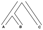
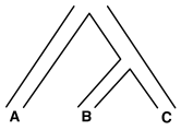
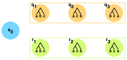
(a)	(b)	(c)

Figure 2: The two parental trees that represent the phylogenetic network of Fig. 1 and the corresponding PhyloNet-HMM. genomic regions that are not of introgressive descent evolve within the branches of the parental tree in (a), whereas genomic regions of introgressive descent evolve within the branches of the parental tree in (b). Regardless of which of the two parental trees a genomic region evolves, the region might still have phylogenetic switching, which is captured by different gene genealogies within the branches of each parental tree. (c) The corresponding PhyloNet-HMM (only states are shown). The three $q$ states correspond to genomic regions whose evolution follows the parental tree in (a), and there is a state for each of the three possible gene genealogies. The three $r$ states correspond to genomic regions whose evolution follows the parental tree in (b), and there is a state for each of the three possible gene genealogies. $s_{0}$ is the start state. See text for emission and transition probabilities.

To account for this case, we propose a hidden Markov model (HMM) for modeling the evolution of the three genomes. The HMM for this simple case would consist of 7 states: a start state $s_{0}$, and six additional states: $q_{i}$ ($1\leq i\leq 3$), corresponding to gene possible gene genealogies within one parental tree, and $r_{i}$ ($1\leq i\leq 3$), corresponding to gene possible gene genealogies within the other parental tree (see Fig. 2(c)). We denote by $g(q_{i})$ and $g(r_{i})$ the gene trees to which states $q_{i}$ and $r_{i}$ correspond, respectively (these gene trees are shown within the states in Fig. 2(c)).

In this model, transition between two $q$ states or two $r$ states corresponds to switching across recombination breakpoints. The probabilities of such transitions have to do with population parameters (e.g., population size, recombination rates, etc.). Transition from a $q$ state to an $r$ state indicates entering a introgressed region, while transition from an $r$ state to a $q$ state indicates exiting an introgressed region. The probabilities of such transitions have to do, in addition, with introgression and evolutionary forces (back-crossing, selection, etc.). Each state emits a triplet of letters that corresponds to a column in the three-genome sequence alignment. The probability of emitting such a triplet can be computed using a standard phylogenetic substitution model [24].

Following the approaches of [12, 25], the transition probabilities in our model do not represent parameters in an explicit evolutionary model of recombination and introgression. Our choice was made to ease analytical representation and to permit tractable computational inference. We contrast our choice with alternative approaches: examples include (in order of increasing tractability of computational inference at the cost of more simplifying assumptions) methods incorporating the coalescent-with-recombination model [26], the sequentially Markovian coalescent-with-recombination model [13] (which adds the single assumption that coalescence cannot occur between two lineages that do not share ancestral genetic material), and the discretized sequentially Markovian coalescent-with-recombination model [27] (which additionally discretizes time).

Assume that the probability of a site (or, locus) in the genome of B being introgressed is $\gamma$, then we follow the model of [11], and use this parameter to constrain the transition probabilities. Assume a site is emitted by state $q_{1}$ and consider the next site. If it is not in an introgressed region, then the HMM should stay in the $q$ states, with probability $1-\gamma$, and if it is in an introgressed region, it should switch, with probability $\gamma$, to an $r$ state. Thus, the transition probability from $q_{1}$ to any other $q_{i}$ ($1\leq i\leq 3$) state is $(1-\gamma)z(q_{i})$ and to any $r_{i}$ ($1\leq i\leq 3$) state is $\gamma z(r_{i})$, where $z(q_{i})$ is the probability of the gene tree $g(q_{i})$ given the parental tree in Fig. 2(a), and $z(r_{i})$ is the probability of the gene tree $g(r_{i})$ given the parental tree in Fig. 2(b). The $z$ quantities are computable under the coalescent using the technique of [28].

If we denote by $S$ the set $\{q_{1},q_{2},q_{3},r_{1},r_{2},r_{3}\}$ of (non-start) states, then a transition from the start state $s_{0}$ to a state $s\in S$ occurs according to the the normalized gene tree probability

$$t_{s}=\frac{z(s)}{\sum\limits_{s^{\prime}\in S}z(s^{\prime})}.$$

For $s\in S$, let $n_{s}=(1-\gamma)z(s)$ and $i_{s}=\gamma z(s)$. Then, the full transition probability matrix, with rows labeled $s_{0},q_{1},q_{2},q_{3},r_{1},r_{2},r_{3}$ and similarly for columns, is

$$\left[\begin{array}[]{ccccccc}0&t_{q_{1}}&t_{q_{2}}&t_{q_{3}}&t_{r_{1}}&t_{r_{2}}&t_{r_{3}}\\ 0&n_{q_{1}}&n_{q_{2}}&n_{q_{3}}&i_{r_{1}}&i_{r_{2}}&i_{r_{3}}\\ 0&n_{q_{1}}&n_{q_{2}}&n_{q_{3}}&i_{r_{1}}&i_{r_{2}}&i_{r_{3}}\\ 0&n_{q_{1}}&n_{q_{2}}&n_{q_{3}}&i_{r_{1}}&i_{r_{2}}&i_{r_{3}}\\ 0&i_{q_{1}}&i_{q_{2}}&i_{q_{3}}&n_{r_{1}}&n_{r_{2}}&n_{r_{3}}\\ 0&i_{q_{1}}&i_{q_{2}}&i_{q_{3}}&n_{r_{1}}&n_{r_{2}}&n_{r_{3}}\\ 0&i_{q_{1}}&i_{q_{2}}&i_{q_{3}}&n_{r_{1}}&n_{r_{2}}&n_{r_{3}}\\ \end{array}\right]$$

Given that

$$\sum_{i=1}^{3}z(q_{i})=\sum_{i=1}^{3}z(r_{i})=1,$$

it follows that the entries in each row of the matrix add up to $1$. Further, the HMM always starts in state $s_{0}$; that is the initial state probability distribution is given by $1$ for state $s_{0}$ and $0$ for every other state.

Once in a state $s\in S$, the HMM emits an observation $O_{t}$ where $1\leq t\leq K$. Emissions occur according to a substitution model $\theta$ (we used the generalized time-reversible (GTR) model [29]), yielding the emission probability

$$e_{s,\theta}(O_{t}) = P[O_{t}|x_{t}=s,\theta]$$

$$= P[O_{t}|g(s),b_{g(s)},\theta],$$

where $b_{g(s)}$ are the branch lengths of the gene tree associated with state $s_{i}$.

The PhyloNet-HMM model: The general case

Modeling a phylogenetic network in terms of a set of parental trees fails for most cases [30]. For example, if two individuals are sampled from species B in Fig. 1, then one allele of a certain locus in one individual may trace the left parent (to C), while another allele of the same locus but in the other individual may trace the right parent (to A). Neither of the two parental trees in Fig. 2 can capture this case. Similarly, if one individual is sampled per species, but multiple introgression events occur or divergence events follow the introgression, the concept of parental trees collapses [11].

To deal with the general case—where multiple introgressions could occur, multiple individuals could be sampled, and introgressed species might split and diverge (and even hybridize again later)—we propose the following approach that is based on MUL-trees [11].

The basic idea of the method is to convert the phylogenetic network $N$ into a MUL-tree $T$ and then make use of some existing techniques to complete the computation on $T$ instead of on $N$. A MUL-tree [31] is a tree whose leaves are not uniquely labeled by a set of taxa. Therefore, alleles of individuals sampled from one species, say $x$, can map to any of the leaves in the MUL-tree $T$ that are labeled by $x$. For network $N$ on taxa ${\mathscr{X}}$, we denote by $A_{x}$ the set of alleles sampled from species $x$ ($x\in{\mathscr{X}}$), and by $c_{x}$ the set of leaves in $T$ that are labeled by species $x$. Then an allele mapping is a function $f:(\cup_{x\in{\mathscr{X}}}A_{x})\rightarrow(\cup_{x\in{\mathscr{X}}}c_{x})$ such that if $f(a)=d$, and $d\in c_{x}$, then $a\in A_{x}$ [32]. Fig. 3 shows an example of converting a phylogenetic network into a MUL-tree along with all allele mappings when a single allele is sampled per species.

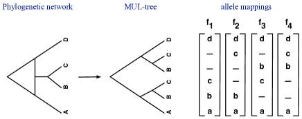
Figure 3: From a phylogenetic network to a MUL-tree. Illustration of the conversion from a phylogenetic network to a MUL-tree, along with all allele mappings associated with the case in which single alleles $a$, $b$, $c$ and $d$ were sampled from each of the four species $A$, $B$, $C$ and $D$, respectively.

The branch lengths and inheritance probabilities $\gamma$ are transferred from the phylogenetic network to the MUL-tree in a straightforward manner (see [11] for details).

Now, two changes to the PhyloNet-HMM given for the simple case above are required. While in the simple case above, we used two classes of states (the $q$ and $r$ states), in the general case, the PhyloNet-HMM will contain $k$ classes of states, where $k$ is the number of all possible allele mappings. As above, the transitions within a class of states corresponds to local phylogeny switching due to recombination and ILS, whereas transitioning between classes corresponds to introgression breakpoints. Second, the transition probabilities are now computed using the method of [11], since the methods of [28, 33] are not applicable to MUL-trees.

Learning the model and conducting inference

We adopted an expectation-maximization (EM) approach to infer model parameters $\lambda$ that maximize the likelihood of the model $P[O_{1},\ldots,O_{K}|\lambda]$. Here, $\lambda$ consists of the (1) parental tree branch lengths, (2) the gene genealogy branch lengths, (3) the substitution model parameters $\theta$, and (4) the parental tree switching probability, $\gamma$. Notice that that $z()$ values are completely determined by the parental tree branch lengths and gene tree topology; hence, they are not free parameters in this model.

The standard forward and backward algorithms [16] were used to compute the model likelihood for fixed $\lambda$. We used Brent’s method [17] as a univariate optimization heuristic during each E-M iteration. To reduce overfitting during optimization, branch length parameters were optimized for each topologically distinct parental tree, and similarly for each topologically distinct unrooted gene genealogy (since we use a reversible substitution model). States therefore “shared” branch length parameters based on topological equivalence of parental trees and gene genealogies.

To evaluate the effectiveness of our optimization heuristic, we utilized different starting points for our E-M search. We found that our heuristics were robust to the choice of starting point since the searches all converged to the same solution (data not shown). We found that the choice of starting point only affected search time.

After model parameter values were inferred using the E-M heuristic, Viterbi’s algorithm [16] was used to compute optimal paths and, thus, annotations of the genomes. More formally, Viterbi algorithm computes the path of states $\pi$ such that

$$\pi\leftarrow{\rm argmax}_{\pi^{\prime}}{\bf P}(x,\pi^{\prime}),$$

where $x$ is the sequence alignment.

Further, the forward and backward algorithms can be used to conduct posterior decoding and assess confidence for the states on a path $\pi$:

$${\bf P}(\pi_{i}=k|x)=\frac{f_{k}(i)b_{k}(i)}{{\bf P}(x)},$$

where $f_{k}(i)$ is the probability of the observed sequence alignment up to and include column $i$, requiring that $\pi_{i}=k$ (computable with the forward algorithm); $b_{k}(i)$ is the probability of the last $L-i$ columns ($L$ is the total number of columns in the alignment), requiring that $\pi=k$ (computable with the backward algorithm); and, ${\bf P}(x)$ is the probability of the alignment (computable with either the forward or backward algorithms).

We will show in the Results section the application of both Viterbi’s algorithm and the posterior decoding in detecting introgression in genomes.

Results/Discussion

We applied the PhyloNet-HMM framework to detect introgression in chromosome 7 in three sets of mice, as described above. Each data set consisted of two individuals from M. m. domesticus and two individuals from M. spretus. Thus the phylogenetic network is very simple, and has only two leaves, with a reticulation edge from M. spretus to M. m. domesticus; see Fig. 4(a).

Figure 4: The phylogenetic network used in our analyses and the two parental trees. The phylogenetic network (a) captures introgression from M. spretus to M. m. domesticus. The red and blue lines illustrate two possible gene genealogies involving no introgression (blue) and introgression (red). The parental tree in (b) captures genomic regions with no introgression, while the parental tree in (c) captures genomic regions of introgressive descent.

Similarly to the example in Fig. 1 and 2, the evolution of lineages within the species network can be equivalently captured by the set of parental trees in Fig. 4(b-c). Since in each data set we have four genomes, there are 15 possible rooted gene trees on four taxa. Therefore, for each data set, our model consisted of 15 $q$ states, 15 $r$ states, and one start state $s_{0}$, for a total of 31 states.

We use our new model and inference method to analyze two types of empirical data sets. The first type includes individuals of known introgressed origin, and our model recovers the introgressed genomic region reported in [2] (Fig. 5(b)). On the other hand, the second type consists of “control” individuals collected from geographically distant regions so as to minimize the chances of introgression (though, it is not possible to rule out that option completely). Our model detected no regions of introgressive descent in this dataset (Fig. 5(e) and (h)).

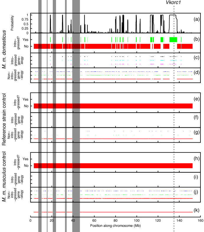
Figure 5: Introgression scans of chromosome 7 from three mouse genome data sets. Mus musculus domesticus samples data set (panels b-d), negative control scans of reference strains data set (panels e-g), and Mus musculus musculus samples (panels h-j). In panels (b), (e), and (h), genomic regions are classified as having introgressed origin or not based on parental-tree switching in a PhyloNet-HMM analysis. Panels (c), (f), and (i) show the rooted gene genealogy inferred for each locus classified as introgressed. Each distinct rooted gene genealogy is represented using a distinct color and row. Panels (d), (g), and (j) show the rooted gene genealogy inferred for the remaining loci (which were not classified as introgressed). Panel (k) shows loci sampled by the Mouse Diversity Array [18], which we used to genotype our samples. The dashed vertical line indicates the location of the Vkorc1 gene, which was shown by [2] to be a driver gene in an introgression event between (M. m. domesticus and Mus spretus) and leading to the spread of rodenticide resistance in the wild. The grey bars indicate regions with missing data. Panel (a) gives the results of posterior decoding on introgressed ($r$) states based on the results in Panel (b); see text for more details.

We ran PhyloNet-HMM to analyze the M. m. domesticus data set, which consisted of samples from a putative hybrid zone between M. m. domesticus and M. spretus (Figure 5(b-d). The data set contained sequences from chromosome 7, the chromosome containing the Vkorc1 gene. Vkorc1 is a gene implicated in the introgression event and the spread of rodenticide resistance in the wild [2].

Based on the pattern of recovered parental trees, the PhyloNet-HMM analysis detected introgression in the vicinity of the Vkorc1 gene from approximately 131 Mb to 138 Mb, reproducing the findings of [2]. The analysis also uncovered recombination and incomplete lineage sorting in the region, as evidenced by incongruence among the rooted gene genealogies that were ascribed to loci.

The PhyloNet-HMM analysis detected introgression in 12.0% of sites in chromosome 7. Notably, the analysis located similar regions in other parts of chromosome 7 which were not investigated by prior studies such as [2]. Examples include the region from 122 Mb to 125 Mb and the region from 113 Mb to 116 Mb. These introgressed regions contain about 300 genes, with two groups with significant gene ontology (GO) term enrichment: one with olfaction-related genes, and the other with immune-response related genes. It is worth mentioning that the method does detect ILS within introgressed regions and outside those regions as well; yet, it does not switch back and forth between these two cases repeatedly (which is an issue that plagues methods that assume independence across loci).

As described by our model above, if we sum the transition probabilities from any $q$ state to all $r$ states, we obtain a value for $\gamma$. We performed this computation for each $q$ state, and took the average of all $\gamma$ estimates based on each of the 15 $q$ states. Our model estimates the value of $\gamma$ as $0.008$. This can be interpreted as the probability of switching due to introgression, and can shed light on introgression parameters.

To assess confidence in these findings, we used a modified version of the posterior decoding. Recall that in our model, there are 15 states corresponding to the parental tree in Fig. 4(c): $r_{1},r_{2},\ldots,r_{15}$. As we are interested in assessing confidence in whether a column $i$ in the alignment $x$ falls within an introgressed region, we computed for column $i$ the quantity

$$p_{i}=\sum_{k\in\{r_{1},\ldots,r_{15}\}}{\bf P}(\pi_{i}=k|x).$$

This quantity, for all positions in chromosome 7, is shown in Fig. 5(a). Clearly, the introgressed regions indicated by green bars in Fig. 5(b) have very high support (close to 1), particularly the region around the Vkorc1 gene. Very few regions detected as introgressed by Viterbi’s algorithm have low support (close to 0.25). However, these regions are very short.

To further validate our approach, we repeated our scans on the reference strain control data set and the M. m. musculus control data set, which contained two sets of mice that were not known to hybridize (Figure 5(e-j)). In combination with the M. spretus samples from the previous scan, one control data set consisted of two individuals from an inbred laboratory strain that were nearly genetically identical, and the other control data set consisted of geographically and genetically distinct samples from M. m. musculus, which is not known to hybridize with M. spretus in the wild.

In both controls, PhyloNet-HMM did not detect introgression. In the M. m. musculus control data set, the analysis recovered signatures of recombination and ILS, based on local incongruence among inferred rooted gene genealogies. The scans of the laboratory strains in the reference strain control data set exhibited less local phylogenetic incongruence compared to the scans of the wild M. m. musculus samples, as expected by the genetic homogeneity of individuals from a single laboratory strain.

Conclusion

In this paper, we introduced a new framework, PhyloNet-HMM, for comparative genomic analyses aimed at detecting introgression. Our framework allows for modeling point mutations, recombination, and introgression, and can be trained to tease apart the effects of incomplete lineage sorting from those of introgression.

We implemented our model, along with standard HMM algorithms, and analyzed a data set of chromosome 7 from four mouse genomes where introgression was previously reported. Our analyses detected the reported introgression with high confidence, and detected other regions in the chromosome as well. Using the model, we estimated that about 12% of the sites in chromosome 7 in the an M. m. domesticus genome are of introgressive descent. Further, we ran the model on negative control data sets, and detected no introgression.

We described above how to extend the model to general data sets with arbitrary hybridization and speciation events, by using a MUL-tree technique. However, as larger (in terms of number of genomes) data sets become available, we expect the problem to become more challenging, particularly in terms of computational requirements. Furthermore, while the discussion so far has assumed that the set of states is known (equivalently, that the phylogenetic network is known), this is not the case in practice. This is a very challenging problem that, if not dealt with carefully, can produce poor results. In this work, we explored a phylogenetic network corresponding to a hypothesis provided by a practitioner. In general, the model can be “wrapped” by a procedure that iterates over all possible phylogenetic network hypotheses, and for each one the model can be learned as above, and then using model selection tests, an optimal model can be selected. However, this is prohibitive except for data sets with very small numbers of taxa. As an alternative, the following heuristic could be adopted instead: first, sample loci across the genome that are distant enough to guarantee that they are unlinked; second, use trees built on these loci to search for a phylogenetic network topology using techniques [34]; third, conduct the analysis as above. Of course, the phylogenetic network identified by the search might be inaccurate, in which case use of an ensemble of phylogenetic networks that are close to that one in terms of optimality may be beneficial.

Appendix

Table 1: Mouse samples and data sets.

Sample name	Origin	Gender	Source	Alias
Spanish-mainland-domesticus	Roca del Valles, Catalunya, Spain	Female	[19]	MWN1287
Georgian-domesticus	Adjaria, Georgia	Male	[19, 21]	DGA
A-spretus	Puerto Real, Cadiz Province, Spain	Male	This study	SPRET/EiJ
B-spretus	Sante Fe, Granada Province, Spain	Unknown	[20]	SEG/Pas
A-reference	Classical	Male	This study	C57BL/6J
B-reference	Classical	Female	[20]	C57BL/6J
A-musculus	Urumqi, Xinjiang, China	Male	[19]	Yu2097m
B-musculus	Hebukesaier, Xinjiang, China	Female	[19]	Yu2120f
Data set	Set of samples used
M. m. domesticus	Spanish-mainland-domesticus, Georgian-domesticus, A-spretus, B-spretus
Reference strain control	A-reference, B-reference, A-spretus, B-spretus
M. m. musculus control	A-musculus, B-musculus, A-spretus, B-spretus

We obtained new mouse samples and also used existing mouse samples from previous studies. The array CEL files for existing mouse samples are available online (http://cgd.jax.org/datasets/diversityarray/CELfiles.shtml and by request from the authors of [20]). The introgression scans examined patterns of local phylogeny switching involving an M. m. domesticus sample from the region of sympatry with two M. spretus strains and a baseline M. m. domesticus sample from far away. The control scans utilized the two M. spretus strains along with two other mice that were known to not have introgressed with M. spretus: either two individuals from the classical laboratory C57BL/6J strain, or two wild M. m. musculus mice.

References

- 1. Mallet J (2005) Hybridization as an invasion of the genome. TREE 20: 229-237.
- 2. Song Y, Endepols S, Klemann N, Richter D, Matuschka FR, et al. (2011) Adaptive introgression of anticoagulant rodent poison resistance by hybridization between old world mice. Current Biology 21: 1296 - 1301.
- 3. The Heliconious Genome Consortium (2012) Butterfly genome reveals promiscuous exchange of mimicry adaptations among species. Nature 487: 94–98.
- 4. Maddison W (1997) Gene trees in species trees. Systematic Biology 46: 523-536.
- 5. Green RE, Krause J, Briggs AW, Maricic T, Stenzel U, et al. (2010) A draft sequence of the Neandertal genome. Science 328: 710-722.
- 6. Eriksson A, Manica A (2012) Effect of ancient population structure on the degree of polymorphism shared between modern human populations and ancient hominids. Proceedings of the National Academy of Sciences 109: 13956-13960.
- 7. Staubach F, Lorenc A, Messer P, Tang K, Petrov D, et al. (2012) Genome patterns of selection and introgression of haplotypes in natural populations of the house mouse (Mus musculus). PLoS Genetics 8: e1002891.
- 8. Moody M, Rieseberg L (2012) Sorting through the chaff, nDNA gene trees for phylogenetic inference and hybrid identification of annual sunflowers (Helianthus sect Helianthus). Molecular Phylogenetics And Evolution 64: 145-155.
- 9. Nakhleh L (2013) Computational approaches to species phylogeny inference and gene tree reconciliation. Trends in Ecology & Evolution : to appear.
- 10. Durand EY, Patterson N, Reich D, Slatkin M (2011) Testing for ancient admixture between closely related populations. Molecular Biology and Evolution 28: 2239-2252.
- 11. Yu Y, Degnan JH, Nakhleh L (2012) The probability of a gene tree topology within a phylogenetic network with applications to hybridization detection. PLoS Genet 8: e1002660.
- 12. Hobolth A, Christensen OF, Mailund T, Schierup MH (2007) Genomic relationships and speciation times of human, chimpanzee, and gorilla inferred from a coalescent hidden Markov model. PLoS Genet 3: e7.
- 13. Dutheil JY, Ganapathy G, Hobolth A, Mailund T, Uyenoyama MK, et al. (September 2009) Ancestral population genomics: The coalescent hidden markov model approach. Genetics 183: 259-274.
- 14. Mailund T, Dutheil JY, Hobolth A, Lunter G, Schierup MH (2011) Estimating divergence time and ancestral effective population size of Bornean and Sumatran orangutan subspecies using a coalescent hidden Markov model. PLoS Genet 7: e1001319.
- 15. Mailund T, Halager AE, Westergaard M, Dutheil JY, Munch K, et al. (2012) A new isolation with migration model along complete genomes infers very different divergence processes among closely related great ape species. PLoS Genet 8: e1003125.
- 16. Rabiner LR (1989) A tutorial on hidden Markov models and selected applications in speech recognition. Proceedings of the IEEE 77: 257–286.
- 17. Brent RP (1973) Algorithms for Minimization without Derivatives. Mineola, New York: Dover Publications, 1–208 pp.
- 18. Yang H, Ding Y, Hutchins LN, Szatkiewicz J, Bell TA, et al. (2009) A customized and versatile high-density genotyping array for the mouse. Nat Meth 6: 663–666.
- 19. Yang H, Wang JR, Didion JP, Buus RJ, Bell TA, et al. (2011) Subspecific origin and haplotype diversity in the laboratory mouse. Nat Genet 43: 648–655.
- 20. Didion J, Yang H, Sheppard K, Fu CP, McMillan L, et al. (2012) Discovery of novel variants in genotyping arrays improves genotype retention and reduces ascertainment bias. BMC Genomics 13: 34.
- 21. Guénet JL, Bonhomme F (2003) Wild mice: an ever-increasing contribution to a popular mammalian model. Trends in Genetics 19: 24-31.
- 22. Scheet P, Stephens M (2006) A fast and flexible statistical model for large-scale population genotype data: Applications to inferring missing genotypes and haplotypic phase. The American Journal of Human Genetics 78: 629 - 644.
- 23. Meng C, Kubatko LS (2009) Detecting hybrid speciation in the presence of incomplete lineage sorting using gene tree incongruence: A model. Theor Popul Biol 75: 35-45.
- 24. Felsenstein J (2004) Inferring Phylogenies. Sinauer Associates, Sunderland, Massachusetts.
- 25. Westesson O, Holmes I (2009) Accurate detection of recombinant breakpoints in whole-genome alignments. PLoS Comput Biol 5: e1000318.
- 26. Husmeier D, Wright F (2004) Detection of recombination in DNA multiple alignments with hidden Markov models. Journal of Computational Biology 8: 401-427.
- 27. Li H, Durbin R (2011) Inference of human population history from individual whole-genome sequences. Nature 475: 493–496.
- 28. Degnan JH, Salter LA (2005) Gene tree distributions under the coalescent process. Evolution 59: 24-37.
- 29. Rodriguez F, Oliver J, Marin A, Medina J (1990) The general stochastic model of nucleotide substitution. Journal of Theoretical Biology 142: 485-501.
- 30. Yu Y, Than C, Degnan J, Nakhleh L (2011) Coalescent histories on phylogenetic networks and detection of hybridization despite incomplete lineage sorting. Systematic Biology 60: 138-149.
- 31. Huber K, Oxelman B, Lott M, Moulton V (2006) Reconstructing the evolutionary history of polyploids from multilabeled trees. Molecular Biology and Evolution 23: 1784-1791.
- 32. Yu Y, Degnan J, Nakhleh L (2012) The probability of a gene tree topology within a phylogenetic network with applications to hybridization detection. PLoS Genetics 8: e1002660.
- 33. Wu Y (2012) Coalescent-based species tree inference from gene tree topologies under incomplete lineage sorting by maximum likelihood. Evolution 66: 763-775.
- 34. Yu Y, Barnett RM, Nakhleh L (2013) Parsimonious inference of hybridization in the presence of incomplete lineage sorting. Systematic Biology 62: 738-751.