On the Origin of the 6.4 keV Line in the Galactic Center Region

Abstract

We analyse the 6.4 keV iron line component produced in the Galactic Center (GC) region by cosmic rays in dense molecular clouds (MCs) and in the diffuse molecular gas. We showed that this component, in principle, can be seen in several years in the direction of the cloud Srg B2. If this emission is produced by low energy CRs which ionize the interstellar molecular gas the intensity of the line is quite small, $<1$%. However, we cannot exclude that local sources of CRs or X-ray photons nearby the cloud may provide much higher intensity of the line from there. Production of the line emission from molecular clouds depends strongly on processes of CR penetration into them. We show that turbulent motions of neutral gas may generate strong magnetic fluctuations in the clouds which prevent free penetration of CRs into the clouds from outside. We provide a special analysis of the line production by high energy electrons. We concluded that these electrons hardly provide the diffuse 6.4 keV line emission from the GC because their density is depleted by ionization losses. We do not exclude that local sources of electrons may provide an excesses of the 6.4 keV line emission in some molecular clouds and even reproduce a relatively short time variations of the iron line emission. However, we doubt whether a single electron source provides the simultaneous short time variability of the iron line emission from clouds which are distant from each other on hundred pc as observed for the GC clouds. An alternative speculation is that local electron sources could also provide the necessary effect of the line variations in different clouds that are seen simultaneously by chance that seems, however, very unlikely.

1 Introduction

The origin of 6.4 keV emission from molecular clouds (MCs) of the Galactic Center (GC) has been discussed from 1993 (see Sunyaev et al., 1993), and it was concluded that this emission was produced by keV photons emitted by Srg A* about 100 yr ago (see e.g. last publications of Inui et al., 2009; Ponti et al., 2010; Terrier et al., 2010; Nobukawa et al., 2011; Capelli et al., 2012; Ryu et al., 2013; Clavel et al., 2013, and references therein). This line emission was observed first in the direction of the cloud Srg B2 (Koyama et al., 1996). The subsequent observations of the line and X-ray continuum emission from this cloud found its prominent time variability whose time characteristic corresponded to the period for which the front of primary photons from Sgr A* crossed the cloud (see e.g. Inui et al., 2009; Terrier et al., 2010). Analysis of the Chandra data provided by Clavel et al. (2013) showed that this activity of SgrA* can be presented as short X-ray flares whose duration is about 10 yr. In principle, past flares of Sgr A* can be found on time scales of ten thousand years (see Cramphorn & Sunyaev, 2002)

For the last ten years the 6.4 keV intensity of Sgr B2 has dropped down in about three times in comparison with its maximum value in 2000 (see Nobukawa et al., 2011). The background 6.4 keV emission for e.g. the cloud Sgr B2 is expected to be seen in several years when the front of primary Sgr A* photons leaves finally the cloud. Does it mean that in several years the line flux from Sgr B2 will drop down to zero?

The 6.4 keV emission from the GC clouds can also be provided by cosmic rays (CRs). Three aspects of the alternative iron line production by CRs have to be clarified:

• It is known that the GC medium is filled by relatively low energy CRs. As Indriolo et al. (2010) showed, CRs of MeV energies ionize the interstellar gas and are absorbed there. The density of these CRs in the GC can be derived from measurements of the absorption line of the ionised molecular hydrogen ($H_{3}^{+}$). Thus, Oka et al. (2005) and Goto et al. (2008, 2011) found an unusually high ionization rate in the GC, which is not observed in other parts of the Galactic Disk. The ionization rate, $\zeta$, is almost uniform throughout of the GC on scales about 200 pc, $\zeta\sim(1-3)\times 10^{-15}$ s^-1. This suggests a single and widespread mechanism of ionization there. Then the question is what is the level of the 6.4 keV line emission produced by these MeV CRs. Alternatively, the background flux of the 6.4 keV line in the GC can also be provided by a hypothetic injection of subrelativistic protons by a star accretion onto the central black hole (see Dogiel et al., 2009a). They estimated this flux for the molecular cloud Sgr B2 and found that in several years it might be about 15% of the maximum observed in 2000. Of course, these predictions are strongly model dependent and cannot be considered as reliable;

• The line emission from several clouds like the Arches cluster region, Sgr C, G0.162-0.217, GO.11-0.11 and others (see Fukuoka et al., 2009; Tsuru et al., 2010; Tatischeff et al., 2012; Yusef-Zadeh et al., 2013a) is unlikely due to photoionization because e.g. some of them do not show any time variability as expected in the photoionization model. The question is whether the line flux from these clouds is produced by background CRs or by CRs from local sources;

• Although the photon origin of the 6.4 keV line emission is widely accepted, Yusef-Zadeh et al. (2013a) developed a model of the line production by relativistic electrons which explained also the flux time variability from the GC clouds.

Below we provide investigations of the iron line generation by CRs in the GC.

2 6.4 keV Emission from Sgr B2 Produced by Subrelativistic Protons

We investigate first the case of ionization by protons. As we noticed above CRs ionize the molecular gas in the GC with the rate $\zeta\geq 3\times 10^{-15}$ s^-1 which is almost constant in the GC region. The rate of ionization by subrelativistic protons reads as

$$\zeta\simeq\int\limits_{I({\rm H_{2}})}^{E_{p}^{\rm max}}dE_{p}\sigma_{p}^{\rm ioni}(E_{p})n_{\rm p}(E_{p})v_{p}(E_{p})~{},$$ (1)

where $\sigma_{p}^{\rm ioni}$ is the cross-sections of ionization by protons taken e.g. from Tatischeff (2003), $n_{\rm p}(E_{p})$ is the spectrum of primary protons, $I({\rm H_{2}})$ is the ionization potentials of hydrogen, $E^{\rm max}_{p}$ is the maximum energy of primary protons, and $v_{p}$ is the velocities of primary protons. As in Dogiel et al. (2013) the contribution from knock-on electrons is neglected.

Parameters of the proton spectrum necessary for the observed ionization rate in the GC, $\zeta=3\times 10^{-15}$ s^-1, can be derived, if we take the proton spectrum as power-law, $n_{p}(E_{p})=KE_{p}^{\gamma}$, where $E_{p}$ is the kinetic energy of protons, $E_{p}=\sqrt{p^{2}c^{2}+(m_{p}c^{2})^{2}}-m_{p}c^{2}$. In Fig. 1 we presented the luminosity of protons in the GC region of the radius 200 pc and thickness 60 pc derived from Eq. (1).

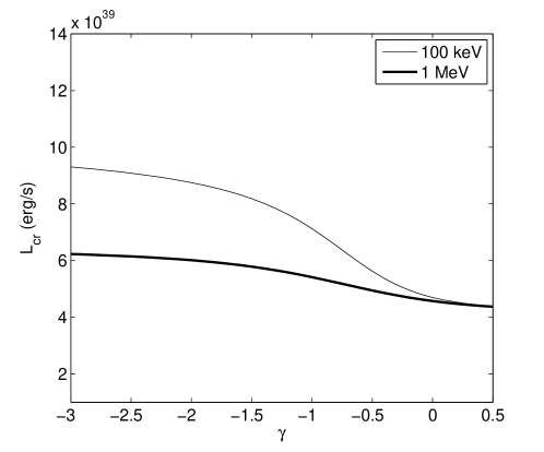
Figure 1: The luminosity of CR protons in the GC region,$L_{cr}$, necessary to provide the ionization rate $\zeta=3\times 10^{-15}$ s^-1 as a function of the proton spectral index $\gamma$. Thick line: for the range of protons 1 - 100 MeV, thin line: the range of protons 100 keV - 100 MeV

We see that the required proton luminosity in the GC region, $\leq 10^{40}$ erg s^-1, seems to be quite reasonable if supplied by SNs in the GC (see Crocker et al., 2011). As Cheng et al. (2007, 2011) and Dogiel et al. (2009c) showed, this luminosity of subrelativistic and relativistic CRs in the GC can also be provided by processes of star accretion onto the central black hole, though as we mentioned these estimates cannot be considered as reliable.

Then for the proton spectrum derived from Eq. (1) we can estimate an expected background level of the 6.4 keV flux from Sgr B2 provided by the protons when the front of Sgr A* photons leaves the cloud. The equation is

$$F_{6.4}\simeq\eta_{Fe}n_{H}V{\int\limits_{I({\rm Fe})}^{E_{p}^{\rm max}}}dE_{p}\sigma_{p}^{\rm Fe}(E_{p})n_{\rm p}(E_{p})v_{p}(E_{p})$$ (2)

where $\sigma_{p}^{\rm Fe}$ is the cross-section of iron ionization by protons (see Tatischeff, 2003), $\eta_{Fe}$ is the iron abundance, $I({\rm Fe~{}K})=7.1$ keV is the ionization potentials of iron, and $V$ is the cloud volume. The total mass of Sgr B2 is poorly known. In the volume of 42 pc diameter this mass ranges from $2\cdot 10^{5}$ to $7\cdot 10^{6}$ M_⊙ (Oka et al., 1998). For estimates we take the mass of $10^{6}$ M_⊙ and the fixed ionization rate in the GC $\zeta=3\times 10^{-15}$ s^-1. The background flux of the 6.4 keV line as a function of proton spectral index $\gamma$ and the minimum energy of protons, $E_{min}$, equaled 1 MeV (thick solid line) and 100 keV (thin solid line) is shown in Fig. 2.

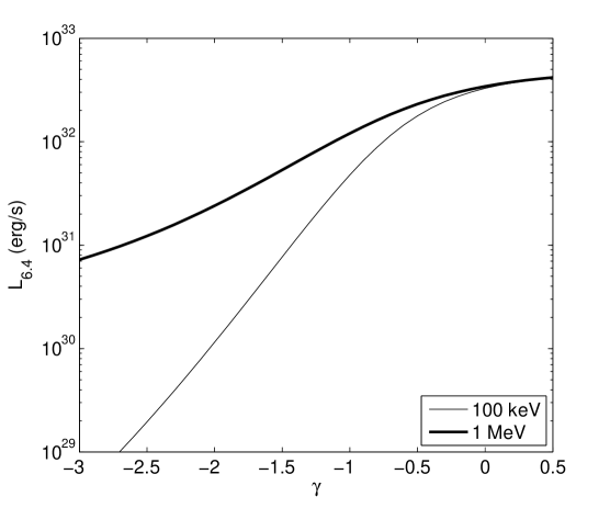
Figure 2: 6.4 keV flux from Sgr B2 generated by protons as a function of their spectral index $\gamma$. The spectrum parameters are the same as in Fig. 1.

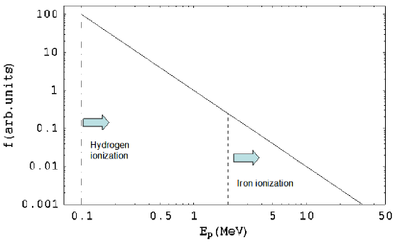
Figure 3: The energy ranges of subrelativistic protons which ionize the hydrogen gas and iron atoms.

For the fixed ionization rate $\zeta$ the expected 6.4 keV flux depends on the spectral index of protons and the cut-off energy of protons $E_{min}$, the steeper is the spectrum and the smaller is $E_{min}$, the less is the expected flux of the diffuse 6.4 keV flux from the GC region. This effect is illustrated in Fig. 3 where we showed the energy range of subrelativistic protons which ionize the hydrogen gas and iron atoms (see for the ionization cross-sections Tatischeff, 2003; Dogiel et al., 2013).

From Fig. 2 we can conclude that for steep spectra of protons we expect further decrease of the flux which will reach the level below $\leq 1$% of its maximal value measured in 2000, if there are no local sources of CRs in the Sgr B vicinity. For $\gamma<0.5$ the flux of background 6.4 keV line emission from Sgr B2 depends strongly on $E_{min}$ of the protons. We see from the figure that this flux is negligible if $E_{min}=100$ keV. This conclusion is in a full agreement with results obtained by Dogiel et al. (2013) (see Fig. 1 in that paper).

A relatively high flux of the 6.4 keV emission from Sgr B2 may mean that accretion processes generate, indeed, high energy subrelativistic protons in the GC as assumed by Dogiel et al. (2009a). In this case the spectrum of protons is extremely hard, $\propto E^{0.5}$, (see Dogiel et al., 2009b) providing a more effective ionization of iron than in the cases of steep proton spectra (see Fig. 2). Alternatively, there may be local sources of CRs or X-ray photons nearby Sgr B2.

3 Structure of magnetic fields inside the clouds and processes of CR propagation there

Although the model of photoionization by Sgr A* photons is widely accepted several molecular clouds in the GC do not fit with this interpretation, e.g. Arches cluster region, G0.162-0.21, GO.13-013 and others. Their fluxes are not time variable and the equivalent width of the 6.4 kev line does not correspond to ionization by photons (see, e.g. Fukuoka et al., 2009; Ponti et al., 2010; Yusef-Zadeh et al., 2013a). A nice example is the molecular cloud nearby the Arches cluster whose 6.4 keV emission may be generated by CRs. Its emission was analysed in details by Tatischeff et al. (2012), who showed that it was most likely produced by subrelativistic ions. Other cases were investigated by Goto et al. (2013) who assumed that molecular clouds in the central few parsecs region of the Galaxy are ionised by protons emitted by Sgr A*. Yusef-Zadeh et al. (2013b) suggested that the 6.4 keV flux from the cloud GO.13-013 is generated by electrons from local sources.

Estimates of the line emission from a molecular cloud depend strongly on the processes of CR penetration into the clouds. There are two limit cases:

• a) when CRs freely penetrate into the clouds. As Kulsrud & Pearce (1969) showed the MHD-waves are damped due to ion-neutral friction. Therefore, e.g. Morfill (1982); Yusef-Zadeh et al. (2013a) assumed that there are no MHD-waves for scattering inside the clouds. Just in this approximation we obtained above the estimations for Sgr B2;

• Another limit case is when a strong magnetic turbulence inside the clouds excited by chaotic motions of the neutral gas prevents CR penetration into the clouds (see Dogiel et al., 1987, 2005; Dogel^′ & Sharov, 1990). In this case the spatial diffusion coefficient inside the clouds, $D_{c}$, is much smaller than in the intercloud medium that leads to a depletion of CR density inside the clouds due to ionization losses and $p-p$ collisions. This effect may be seen from $\gamma$-ray observations of nearby molecular clouds (see Neronov et al., 2012) . Then the CR distribution in the clouds requires special calculations, as was done e.g. in Dogiel et al. (2009a). Below we discuss this case in more detail and take parameters of the Arches complex as an example.

The diffusion coefficient inside the clouds, $D_{c}$ is determined by the spectrum of magnetic fluctuations excited there. From observations it follows that the neutral gas of the clouds is strongly turbulent. The speed of turbulent motions reaches about 10 km s^-1. The turbulence has a power-law Kolmogorov-like spectrum in a very broad range of scales from supersonic Larson (1981) to subsonic Myers (1983) regions (see also the review of Hennebelle & Falgarone, 2012):

$$v(L)=1.1~{}L^{\alpha}(pc)~{}\mbox{km s${}^{-1}$ where $\alpha\simeq 0.3\div 0.5$}$$ (3)

where $v$ is the velocity of turbulent motions and $L$ is its scale ($0.01<L<300$ pc).

Though the ionization degree in the clouds is small, $x_{e}\leq 10^{-4}$, motions of the neutral gas component generate a turbulence of the ionized gas by friction, and thus excite fluctuations of magnetic fields. The system of equations for fluctuations of the ionized component velocity $u$ and magnetic fields $B$ is

$$\left({{\partial\textbf{u}}\over{\partial t}}+(\textbf{u}\cdot\nabla)\textbf{u}\right)={1\over\rho_{\rm i}}\left[-\nabla P_{\rm i}+{{\left(\nabla\times\textbf{B}\right)\times\textbf{B}}\over{4\pi}}\right]+\nu_{\rm i}\nabla^{2}\textbf{u}+$$

$$+{{\nu_{\rm i}}\over 3}\nabla\nabla\cdot\textbf{u}-\mu_{\rm in}(\textbf{u}-\textbf{v})\,,$$

$${{\partial\textbf{B}}\over{\partial t}}=\nabla\times(\textbf{u}\times\textbf{B}),~{}~{}{{\partial{\rho}}\over{\partial t}}+\nabla\cdot(\rho\textbf{u})=0,~{}~{}\nabla\cdot\textbf{B}=0\,,$$ (4)

where $v$ is the turbulent velocity of the neutral gas, $\rho_{\rm i}$, $\nu_{\rm i}$ etc. are characteristics of the ionized fraction of the gas and $\mu_{\rm in}$ is the frequency of collision between ionized ions and neutral hydrogen.

This set of equations was analysed by Dogiel et al. (1987, 2005) who showed that the energy of magnetic field fluctuations is concentrated at small scales ($L_{\nu}\sim 10^{13}$ cm) where dissipation processes are essential. In this case propagation of magnetized relativistic charged particles along spaghetti-like magnetic field lines can be described as diffusion with the coefficient $D_{c}\sim\pi cL_{\nu}/6$.

Later Istomin & Kiselev (2013) provided a more accurate analysis of these equations and took into account the influence of a large scale magnetic field onto the spectrum of magnetic turbulence. They assumed that magnetic field consists of a large scale average field and small scale magnetic fluctuations ${\bf B}=\textbf{B}_{0}+\textbf{b}$ and $\textbf{B}_{0}={const}$. For the correlator of magnetic fluctuations

$$\langle b_{i}(\textbf{x},t)b_{j}(\textbf{x+r},t)\rangle=2Q(r)\delta_{ij}+rQ^{\prime}(r)\left(\delta_{ij}-\frac{r_{i}r_{j}}{r^{2}}\right)$$ (5)

Istomin & Kiselev (2013) derived the equation which is

$$\frac{1}{2\tau_{\rm c}}\frac{\partial Q(r)}{\partial t}=\left[V(0)-V(r)+\frac{1}{\pi\rho_{\rm i}\mu_{\rm in}\tau_{\rm c}}\left(Q(0)+\frac{B_{0}^{2}}{6}\right)\right]\times$$

$$\left(Q^{\prime\prime}+\frac{4Q^{\prime}}{r}\right)-V^{\prime}Q^{\prime}-\frac{1}{r}\left(4V^{\prime}+rV^{\prime\prime}\right)\left(Q+\frac{B_{0}^{2}}{6}\right)$$ (6)

where $V(r)$ is a paired correlation function of turbulent velocities of neutral gas

$$\langle v_{i}(\textbf{x},t)v_{j}(\textbf{x+r},\bar{t})\rangle=$$

$$\left(2V(r)\delta_{ij}+rV^{\prime}(r)(\delta_{ij}-\frac{r_{i}r_{j}}{r^{2}})\right)\tau_{\rm c}\delta(t-\bar{t})$$ (7)

Here $f^{\prime}$ means $df/dr$ etc.

Figure 4: Correlation length of magnetic fluctuations $L_{corr}/L_{c}$ against the value of parameter $\beta$

Numerical calculations of Istomin & Kiselev (2013) showed that for small values of $B_{0}$ such as the parameter $\beta=B_{0}/(\tau_{c}\rho_{i}\mu_{in}v^{2})^{0.5}<<1$, the correlation length of magnetic fluctuations, $L_{corr}$, is much smaller than the cloud size $L_{c}$ (see Fig. 4) i.e. the energy of magnetic fields is concentrated at scales much smaller than the cloud size, and the structure of magnetic fields lines is strongly tangled. For typical clouds $L_{c}=1pc$, $v=1$ km s^-1, $n_{H}=10^{4}$cm^-3, $n_{i}=10^{-3}$cm^-3 - neutral and ion densities. For the gas density in the range from $10^{2}$ to $10^{6}$ cmC^-3 the magnetid field strength is in the limits from $B_{0}\sim 30\,\mu G$ to almost $1$ mG (see Crutcher et al., 2010). Then we obtain $\beta\leq 0.1$ and for the diffusion coefficient of CRs in the clouds we have $D_{c}\sim 10^{26}$cm²s^-1 i.e. $D_{c}<<D_{0}$, where $D_{0}\simeq 10^{28}-10^{29}$ cm²s^-1 is the spatial diffusion coefficient in the intercloud medium (see e.g. Berezinsky et al., 1990).

4 Hydrogen and iron ionization by CR protons inside molecular clouds

Using these parameters of CR propagation in molecular clouds we estimate the rate of ionization by protons for the Arches molecular complex as an example. The question is whether the observed iron emission from the Arches cluster region is produced:

1. by background CRs which ionise the diffused molecular gas in the GC,

2. or by CRs from local sources nearby the cloud.

For these two cases CR distribution, ${N}_{p}(E,x)$, inside the cloud can be described by the equation

$$\frac{\partial}{\partial E}\left(b(E)N_{p}\right)-D_{c}\frac{\partial^{2}}{\partial x^{2}}N_{p}=0\,,$$ (8)

whose rate of energy loses is determined by the ionization , which for subrelativistic protons can be taken in the form

$$\left(\frac{dE}{dt}\right)_{i}\equiv b(E)=-\frac{2\pi ne^{4}}{mc\beta(E)}\ln\Lambda(E)\,.$$ (9)

where $m$ is the electron mass, $v$ is the proton velocity, $\beta=v/c$, $\ln\Lambda$ is the Coulomb logarithm, and $x$ is the coordinate from the cloud surface to the cloud center.

The boundary conditions on the cloud surface ($x=0$) for these case are different:

$$N|_{x=0}=n_{c}(E)$$ (10)

in the case 1. Here $n_{c}(E)$ is the density of background protons, and

$$\left.\frac{\partial N}{\partial x}\right|_{x=0}=Q(E)$$ (11)

in the case 2, where $Q(E)$ is the luminosity of local CR sources at the cloud surface. In the both cases the second boundary condition is taken as

$$N|_{x=\infty}=0$$ (12)

For the time of energy losses

$$\tau_{c}(E,E_{0})=\int\limits_{E_{0}}^{E}\frac{dt}{b(t)}\,.$$ (13)

where $E_{0}$ is the initial energy of a particle, Eq. (8) can be transformed to the standard diffusion equation

$$\frac{\partial}{\partial\tau}\left(N^{\prime}\right)-D_{c}\frac{\partial^{2}}{\partial x^{2}}N^{\prime}=0\,,$$ (14)

where $N^{\prime}=\mid b(E)\mid N_{p}$. Solutions for these two cases can be obtained with the Green function presented e.g. in Morse & Feshbach (1953).

In the simplest case of free penetration the ionization rate in the Arches cloud can be estimated from the observed 6.4 keV flux which is $F_{6.4}=8.5\times 10^{-6}$ ph cm^-2s^-1. As in Tatischeff et al. (2012) we take for the estimates: the total mass of the gas equaled $6\times 10^{4}$ M_⊙, and the gas column density about $L_{H_{2}}\sim 10^{23}$cm^-2. With these parameters we obtain that the ionization rate inside the cloud is about $\zeta_{c}\leq 10^{-13}$ s^-1, i.e. the density of CR protons inside the Arches cloud should be in about 30 - 100 times higher than the CR background in the GC derived from the $H_{3}^{+}$ absorption lines. Thus, the 6.4 keV flux from the cloud is provided by CRs from nearby local sources.

If fluctuations of magnetic field prevent CR free penetration into the cloud, the particles fill the region about $x_{c}\sim\sqrt{D_{c}\tau(E)}$ nearby the cloud surface. Here $D_{c}$ is the diffusion coefficient inside the cloud. As numerical calculations show, the estimate of ionization rate inside the Arches cloud is absolutely the same as for the case of uniform CR density there, if $D_{c}=10^{28}$ cm²s^-1, i.e. protons fill almost uniformly the cloud volume. But if $D_{c}$ is as small as $10^{25}$ cm²s^-1, the CR density is strongly nonuniform in the cloud. The local ionization rate near the cloud surface is about $\zeta\sim 10^{-12}$s^-1 and drops to zero away from the surface. The ionization rate averaged over the cloud volume (that is observed from the IR absorption lines) is in this case about $\bar{\zeta}\sim 5\times 10^{-14}$s^-1.

Thus we conclude that local sources of CR protons/nuclei generate the observed 6.4 keV flux from the Arches molecular complex. The required luminosity of local CR sources (the lower limit in the thick target approximation) can be estimated as

$$L_{CR}(E>10~{}\mbox{MeV})\geq 4\pi R^{2}\frac{F_{6.4}}{\sigma_{Fe}\eta v}\left(\frac{dE}{dt}\right)_{i}\sim 10^{39}\mbox{erg s${}^{-1}$}\,,$$ (15)

where $F_{6.4}$ is the flux of 6.4 keV line from Arches, $E_{X}=6.4$ keV, $R=8$ kpc is the distance between the GC and Earth, $\eta$ is the iron abundance, $v$ is the proton velocity, $\sigma_{Fe}$ is cross-sections of iron ionization, respectively. The spectrum of CRs was supposed to be power-law, $E^{-2}$. We notice that this estimate is correct for the boundary condition (11) but not for (10)

The estimate (15) is in agreement with obtained by Tatischeff et al. (2012). We notice that a quite high luminosity of subrelativistic CRs is required in order to produce the line flux from the region of $\sim 3$ pc diameter.

5 Ionization by CR electrons in the intercloud medium, stationary component

We investigate separately the electron origin of the stationary component of the 6.4 keV line from the diffuse molecular gas in the GC region and the origin of the time-variable component from dense molecular clouds.

As Yusef-Zadeh et al. (2007) showed, there was a correlation between the spatial distribution of radio emission and the molecular gas in the GC. Parameters of the electron spectrum in the GC region can be estimated from the observed flux of radio emission produced by synchrotron losses of relativistic electrons. Yusef-Zadeh et al. (2013a) assumed that these electrons ionize diffuse hydrogen gas and generate also the 6.4 keV line. As follows from Oka et al. (2005) the rate of ionization is almost constant throughout the GC region; this means an almost uniform distribution of the electrons there.

Yusef-Zadeh et al. (2013a) derived parameters of these electrons from the observed nonthermal radio flux from the GC region $2^{\circ}\times 0.85^{\circ}$. The flux is about $\Phi_{\nu}\simeq 2450$ Jy at 325 MHz and the radio spectrum is $\nu^{-0.25}$ at frequencies $\nu<3.3$ GHz. They assumed that the spectrum of radioemitting electrons could be extrapolated into the region 100 keV - 1 GeV, and just the electrons with $E<1$ GeV ionized the GC molecular gas with the rate $\zeta\sim(1-3)\times 10^{-15}$ s^-1; this about the value derived by (see Oka et al., 2005). Then the question is whether these electrons can provide the diffuse 6.4 keV emission in the GC as observed by Uchiyama et al. (2012).

Parameters of the electron spectrum in the form $N_{e}(E)=KE^{-\gamma}$ can be estimated from the observed radio flux $\Phi_{\nu}$ (see e.g. Berezinsky et al., 1990)

$$\Phi_{\nu}=a(\gamma){e^{3}\over{mc^{2}}}\left({{3e}\over{4\pi m^{3}c^{5}}}\right)^{\frac{\gamma-1}{2}}\frac{VKH_{\perp}^{\frac{\gamma+1}{2}}}{R^{2}}\nu^{-\frac{\gamma-1}{2}}$$ (16)

where the constant $a(\gamma)=0.15$ for the electron spectral index $\gamma=1.5$, $V$ is the volume of $2^{\circ}\times 0.85^{\circ}$ GC region, $R\simeq 8$ kpc is the distance from the Sun to the GC, $H$ is the magnetic field strength in the GC. The values of $\nu$ and $\Phi_{\nu}$ are given above. For the magnetic field strength $H=10^{-5}$ G electrons with the energy $E\simeq 2.7$ GeV radiate at the frequency $\nu=325$ MHz.

However, the procedure of extrapolation is not trivial because the electron spectrum is determined by processes of their injection and energy losses. For the GC region filled with the diffuse molecular gas ($n=100$ cm^-3) and the magnetic field ($H=10^{-5}$ G) the synchrocompton losses are significant for energies above 250 GeV. Below this energy electrons lose their energy by bremsstrahlung and then by ionization at $E$ below 350 MeV. Therefore, for $E<250$ GeV we take the rate of energy losses in the form

$$\frac{dE}{dt}\equiv b_{0}(E)=\left(\frac{dE}{dt}\right)_{i}+\left(\frac{dE}{dt}\right)_{br}$$ (17)

The lifetime of electrons $T$ in the GC region is shown in Fig. 5.

Figure 5: The lifetime of electrons for the gas density $n_{H}=10^{4}$cm^-3. The lifetime of electrons is determined by ionization losses up to $E=350$ MeV. Above these energies electrons lose their energy by bremsstrahlung

In the most favorite case for the electron model of the GC ionization, electrons lose all their energy in the GC i.e. processes of electron escape from there are insignificant. Then the kinetic equation for the electron distribution function $f_{e}$ in the GC reads as

$$\frac{d}{dE}\left(b_{0}(E)f_{e}\right)=Q(E)$$ (18)

If the source function $Q(E)$ is power-law, $Q(E)=Q_{0}E^{-1.5}$ as derived from the radio data (the bremsstrahlung losses do not change the injection spectral index), then from Eqs. (16) - (18) we obtain the electron spectrum in the GC as shown in Fig. 6 by the solid line. The extrapolation of Yusef-Zadeh et al. (2013a) is shown in Fig. 6 by the dashed-dotted line.

Figure 6: The spectrum of electrons in the GC (solid line) as derived from Eq. (18). By the dashed-dotted line the extrapolation of electron spectrum into the range below 1 GeV with the spectral index $\gamma=1.5$ derived from the radiodata by Yusef-Zadeh et al. (2013a).

One can see that both the spectra are the same in the range of radioemitting electrons, i.e. above 1 GeV but below this energy they differ strongly from each other. Therefore, it is not surprising that the ionization rate calculated from Yusef-Zadeh et al. (2013a) approximation is about $\zeta\simeq 10^{-15}$ s^-1, while the ionization rate calculated from the spectrum derived from the kinetic equation (18) is only $\zeta\simeq 10^{-17}$ s^-1.

In this respect it is difficult to imagine that ionization by electrons can provide the necessary ionization rate of hydrogen and the diffuse flux of the 6.4 keV line in the interstellar GC region because the intensity of electrons in the energy range $<1$ GeV is strongly depleted by the ionization losses. Therefore we conclude that the electrons are unable to provide the necessary rate of ionization in the GC region, and especially the necessary intensity of the 6.4 keV line from there (see Dogiel et al., 2013).

6 Ionization by CR electrons in molecular clouds, time-variable emission

Low energy electrons lose their energy effectively by ionization losses. Thus, the lifetime of 100 keV electrons is about 10 years (see Fig. 5). This is about of the observed time variability of the 6.4 keV line and continuous emissions from some of the GC molecular clouds. In this respect the electron model can be considered as quite reasonable for local production of a flux of the 6.4 keV line from some of molecular clouds (see Yusef-Zadeh et al., 2013b) and even for interpretation of time variability of this flux as assumed by Yusef-Zadeh et al. (2013a). The question is whether this model is able to explain the observed simultaneous variability of the 6.4 keV emission with the characteristic time about $\geq 10$ yr for the clouds which are at distances about 100 pc from each other as follows from the analyses of Ponti et al. (2010); Ryu et al. (2013) and Clavel et al. (2013). It seems incredible that this simultaneous variability is due to independent local sources of electrons nearby the clouds. From the variability correlation we assume that there is a single time-variable source of electrons in the GC. As a source of electrons we can assume a SNR which emits electrons for about 3000 yr.

First, we mention an advantage of the photon model (see Introduction). Photons propagate along straight lines with the light speed. If a source of photons emits them for a finite period, then these photons provide an increase and decrease of the 6.4 keV line flux from a molecular cloud when the leading and back fronts of the photon flux cross the cloud. Since the effect of photon scattering is negligible the photons can provide the same short-time simultaneous variations of the line emission in distant from each other regions long after their ejection.

Unlike photons, CR propagation in the interstellar magnetic fields is described as diffusion due to scattering on magnetic fluctuations (see e.g. Berezinsky et al., 1990). Even for the diffusion coefficient as large as $D=10^{29}$ cm²s^-1 it takes about $\geq 10^{4}$ yr in order to reach a distance about 100 pc from the source. In the gas with the density $n=100$ cm^-3 only electrons with the initial energy $E\geq 10$ MeV can propagate over this distance (see Fig. 5).

We can present a source of electrons in the form

$$Q(E,\textbf{r},t)=KE^{-\gamma}\delta(\textbf{r})\theta(t)\theta(T-t)\,,$$ (19)

where $K$ is a constant, for the period of source activity we take $T=10$ yr that is most favourable injection time for the electron model, and $\theta(x)$ is the Heaviside step-function.

The non-stationary diffusion equation for electron has the form

$$\frac{\partial f_{e}}{\partial t}-\nabla D\nabla f_{e}+\frac{\partial}{\partial E}\left(b_{0}(E)f_{e}\right)=Q(E,\textbf{r},t)$$ (20)

where $b_{0}(E)$ is given by Eq. (17). The general solution of this equation was obtained by Syrovatskii (1959) (see also Berezinsky et al., 1990). This solution reads as

$$f_{e}(E,\textbf{r},t)=\frac{K}{\mid b_{0}(E)\mid}\int\limits_{E}^{E_{max}}dE_{0}\frac{E_{0}^{-\gamma}}{(4\pi D\tau(E,E_{0}))^{3/2}}\times$$

$$\exp\left[-\frac{\textbf{r}^{2}}{4D\tau(E,E_{0})}\right]\theta(\triangle t+T-\tau(E,E_{0}))\theta(\tau(E,E_{0})-\triangle t)$$ (21)

where $\triangle t$ is the time after the moment when the source ceases particle ejection, $b_{0}(E)$ is described by Eq. (17), $E_{max}$ is maximum energy of ejected electrons and,

$$\tau(E,E_{0})=\int\limits_{E_{0}}^{E}\frac{dz}{b_{0}(z)}\,.$$ (22)

From the solution (21) we can calculate a time-variable flux of the 6.4 keV line from a cloud which is at the distance 100 pc from the electron source

$$F_{6.4}^{e}(r=100~{}\mbox{pc},t)\simeq\eta_{Fe}n_{H}V\int\limits_{E_{e}}dE_{e}\sigma_{e}^{\rm Fe}(E_{e})f_{e}(E_{e},r=100~{}\mbox{pc},t)v_{e}$$ (23)

where $\sigma_{e}^{\rm Fe}$ is the cross-section of iron ionization by electrons (see Tatischeff, 2003), $\eta_{Fe}$ is the iron abundance, and $V$ is the cloud volume.

The results of calculations are shown in Fig. 7 for different values of $E_{max}$. As one can see from the figure the characteristic time of the line variations is $\geq 1000$ yr and does not reproduce the situation presented e.g. in Ponti et al. (2010).

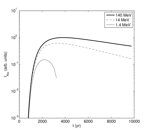
Figure 7: The flux of the 6.4 keV line at the distance 100 pc from the source for different maximum energy of ejected electrons $E_{max}$.

In this respect we find that the model of ionization by electrons has problems to explain the observed time variations of the 6.4 keV flux from the GC clouds.

7 Conclusion

The conclusions can be itemized as follows:

• We conclude that CRs may provide a background level of the 6.4 keV emission in the GC molecular clouds even when the front of photons ejected by Sgr A* leaves them. The density of CRs in the GC region can be estimated from the ionization rate of hydrogen in the GC which is derived from the observed IR absorption lines of $H_{3}^{+}$. The expected background level of the line emission from e.g. the cloud Sgr B2 depends on the spectral index of subrelativistic CRs and it is quite small for steep CR spectra, $<1$% of its maximum in 2000. If in several years this background level is higher than this value, then the reason may be due to ejection of protons by accretion onto the central black hole or other local sources of CRs or photons;

• Local sources of CRs may provide an excess of the 6.4 keV line emission in some of the GC molecular clouds. The required density of CRs depends strongly on processes of particle penetration into the clouds. The analysis of magnetic fields inside the clouds shows that strong small scale magnetic fluctuations may excite there by the turbulence of neutral gas, which prevents free penetration of charged particles into the clouds. Therefore CRs distribution there is strongly nonuniform. However, the CR luminosity of local sources needed for e.g. the observed 6.4 keV flux from the Arches complex is independent of how CRs are distributed there, and equals about $10^{39}$ erg s^-1;

• Our earlier analysis (Dogiel et al., 2013) showed that ionization of the diffuse hydrogen is provided by subrelativistic protons while the diffuse 6.4 keV line in the GC is generated by X-ray photons emitted by Sgr A*. An alternative interpretation was suggested by Yusef-Zadeh et al. (2013a) who assumed that the ionization is provided by background electrons with $E<1$ GeV whose spectrum was extrapolated from the radio data. We showed that the model of ionization by electrons is problematic because the intensity of electrons in the range $<1$ GeV is strongly depleted by ionization losses. However, we cannot exclude (rather arbitrarily) an upturn of the injection spectrum of electrons in the range below 1 GeV . Then one may expect a higher ionization rate in the GC than estimated in section 5. In any case, the local electron spectrum near a very compact region nearby the cloud GO.13-013 derived by Yusef-Zadeh et al. (2013b) from the radio data from 74 to 327 MHz, $\sim E_{e}^{-3.6}$, is much steeper than derived by Yusef-Zadeh et al. (2013a) from the diffuse radio emission in the GC. However. the analysis of Yusef-Zadeh et al. (2013b) showed strong spatial variations of the electron spectral index in this region, and it is unlikely to assume this spectrum in the whole GC region;

• In our opinion another problem of the electron interpretation is a relatively high luminosity of electrons needed for hydrogen ionization in the GC region. As Yusef-Zadeh et al. (2013a) showed the energy supply of electrons necessary for the 6.4 keV line flux from the GC is about $10^{41}$ erg s^-1 that is one order of magnitude higher than the total CR luminosity in the Galaxy and three orders of magnitude higher than the total electron luminosity of the Galaxy (see Strong et al., 2010). It seems that there are no known sources which are able to sustain such an electron population throughout the Central Molecular Zone (CMZ);

• We do not exclude that local sources of electrons may provide an excesses of the 6.4 keV line emission in some molecular clouds and even reproduce a relatively short time variations of the iron line emission ($\sim 10$ yr) (see Yusef-Zadeh et al., 2013a, b). However, if interpretation of the 6.4 keV time variability of e.g Ponti et al. (2010); Ryu et al. (2013); Clavel et al. (2013) is correct, then the electron model is unable to reproduce the simultaneous short time variability of the iron line emission from clouds which are distant from each other by  hundred pc. Alternatively we can speculate that a random distribution of local electron sources could also provide the necessary effect of the line variations in different clouds that are seen by chance. However, this interpretation seems to be very unlikely.

• In our opinion the photon model of Ponti et al. (2010); Ryu et al. (2013); Clavel et al. (2013) reproduces naturally these spatial and temporal characteristics of the 6.4 keV emission in the GC. The photon model has two important advantages: the front of primary photons occupies a very extended region 100 yr after the explosion, and its spatial distribution may have very sharp leading and back fronts that reproduces easily the 10 yr temporal variations of the 6.4 keV emission from GC molecular clouds.

References

- Berezinsky et al. (1990) Berezinsky, V.S., Bulanov, S.V., Dogiel, V.A., Ginzburg, V.L., & Ptuskin, V.S.: 1990, Astrophysics of Cosmic Rays, (ed.V.L.Ginzburg), North Holland.
- Capelli et al. (2012) Capelli, R., Warwick, R. S., Porquet, D., Gillessen, S., & Predehl, P. 2012, A&A, 545, 35
- Cheng et al. (2007) Cheng, K.-S., Chernyshov, D. O. & Dogiel, V. A. 2007, A&A, 473, 351.
- Cheng et al. (2011) Cheng, K.-S., Chernyshov, D. O., Dogiel, V. A., Ko, C.-M., & Ip, W.-H. 2011, ApJ, 731, L17
- Clavel et al. (2013) Clavel, M., Terrier, R., Goldwurm, A. et al. 2013, arXiv1307.3954
- Cramphorn & Sunyaev (2002) Cramphorn, C. K. & Sunyaev R. A. 2002, A&A, 389, 252
- Crocker et al. (2011) Crocker, R. M., Jones, D. I., Aharonian, F. et al. 2011, MNRAS, 413, 763
- Crutcher et al. (2010) Crutcher, R.M., Wandelt, B., Heiles, C., Falgarone, E., & Troland, T.H. 2010, ApJ, 725, 466
- Dalgarno et al. (1999) Dalgarno, A., Yan, M., & Liu, W.-H. 1999, ApJS, 125, 237
- Dogiel et al. (1987) Dogiel, V. A., Gurevich, A. V., Istomin, Ia. N., & Zybin, K. P. 1987, MNRAS, 228, 843
- Dogel′ & Sharov (1990) Dogel′, V. A. & Sharov, G. S. 1990, A&A, 229, 259
- Dogiel et al. (2005) Dogiel, V. A., Gurevich, A. V., Istomin, Ya. N., & Zybin, K. P. 2005, Ap&SS, 297, 201
- Dogiel et al. (2009a) Dogiel, V., Cheng, K.-S., Chernyshov, D. et al. 2009a, PASJ, 61, 901
- Dogiel et al. (2009b) Dogiel, V., Chernyshov, D., Yuasa, T. et al. 2009b, PASJ, 61, 1099
- Dogiel et al. (2009c) Dogiel, V. A., Tatischeff, V., Cheng, K. S. et al. 2009c, A&A, 508, 1
- Dogiel et al. (2011) Dogiel, V., Chernyshov, D., Koyama, K., Nobukawa, M., & Cheng, K.-S. 2011, PASJ, 63, 535
- Dogiel et al. (2013) Dogiel, V., Chernyshov, D., Tatischeff, V., Cheng, K.-S., & Terrier, R. 2013, ApJL, 771, 43
- Fukuoka et al. (2009) Fukuoka, R., Koyama, K., Ryu, S. G., & Tsuru Go, T. 2009, PASJ, 61, 593
- Geballe (2012) Geballe, T. R. 2012, Phil. Trans. R. Soc. A 370, 5151
- Goto et al. (2008) Goto, M., Usuda, T., Nagata, T. et al. 2008, ApJ, 688, 306
- Goto et al. (2011) Goto, M., Usuda, T. Geballe, Th. R. 2011, PASJ, 63, L13
- Goto et al. (2013) Goto, M., Indriolo, N., Geballe, T. R., & Usuda, T. 2013, arXiv1305.3915
- Hennebelle & Falgarone (2012) Hennebelle, P. & Falgarone, E. 2012, A&ARv, 20, 55
- Indriolo et al. (2010) Indriolo, N., Blake, G. A., Goto, M., et al. 2010, ApJ, 724, 1357
- Inui et al. (2009) Inui, T., Koyama, K., Matsumoto, H., & Tsuru Go, T. 2009, PASJ, 61, 241
- Istomin & Kiselev (2013) Istomin, Ya. N. & Kiselev, A. M. 2013, arXiv1309.6110
- Koyama et al. (1996) Koyama, K., Maeda, Y., Sonobe, T. et al. 1996, PASJ, 48, 249
- Kulsrud & Pearce (1969) Kulsrud, R. & Pearce, W. P. 1969, ApJ, 156, 445
- Larson (1981) Larson, R. B. 1981, MNRAS, 194, 809
- Morfill (1982) Morfill, G. E. 1982, ApJ, 262, 749
- Morse & Feshbach (1953) Morse, P. M., & Feshbach, H. 1953, Methods of theoretical physics, International Series in Pure and Applied Physics (New York: McGraw-Hill)
- Myers (1983) Myers, P. C. 1983, ApJ, 270, 105
- Neronov et al. (2012) Neronov, A., Semikoz, D. V. & Taylor, A. M. 2012, PhRvL, 108e1105
- Nobukawa et al. (2011) Nobukawa, M., Ryu, S. G., Tsuru Go, T., & Koyama, K. 2011, ApJL, 739, L52
- Oka et al. (1998) Oka, T., Hasegawa, T., Hayashi, M., Handa, T., & Sakamoto, S. 1998, ApJ, 493, 730
- Oka et al. (2005) Oka, T., Geballe, Th. R., Goto, M., Usuda, T., & McCall, B. J. 2005, ApJ, 632, 882
- Oka (2006) Oka, T. 2006, PNAS, 103, 12235
- Ponti et al. (2010) Ponti, G., Terrier, R., Goldwurm, A., Belanger, G., & Trap, G. 2010, ApJ, 714, 732
- Ryu et al. (2013) Ryu, S. G., Nobukawa, M., Nakashima, S. et al. 2013, PASJ, 65, 33
- Strong et al. (2010) Strong, A. W., Porter, T. A., Digel, S. W. et al. 2010, ApJ, 722, L58
- Sunyaev et al. (1993) Sunyaev, R. A., Markevitch, M., & Pavlinsky, M. 1993, ApJ, 407, 606
- Syrovatskii (1959) Syrovatskii, S. I. 1959, Soviet Astronomy, 3, 22
- Tatischeff (2003) Tatischeff, V. 2003, EAS, 7, 79
- Tatischeff et al. (2012) Tatischeff, V., Decourchelle, A., & Maurin, G. 2012, A&A, 546, 88
- Terrier et al. (2010) Terrier, R., Ponti, G., Belanger, G. et al. 2010, ApJ, 719, 143
- Tsuru et al. (2010) Tsuru, T. G., Uchiyama, H., Nobukawa, M. et al. 2010, astro-ph 1007.4863
- Uchiyama et al. (2012) Uchiyama, H., Nobukawa, M., Tsuru Go, T., & Koyama, K. 2012, PASJ 65, 19
- Yusef-Zadeh et al. (2007) Yusef-Zadeh, F., Wardle, M. & Roy, S. 2007, ApJ, 656, 847
- Yusef-Zadeh et al. (2013a) Yusef-Zadeh, F., Hewitt, J. W., Wardle, M. et al. 2013a, ApJ, 762, 33
- Yusef-Zadeh et al. (2013b) Yusef-Zadeh, F., Wardle, M., D. Lis, D. et al. 2013b, JPCA, 117, 9404