A note on dark matter and dark energy

Abstract

Since the geometry of our universe seems to depend very little on baryonic matter, we consider a variational principle involving only dark matter and dark energy which in addition make them depend on each other. There are no adjustable parameters or scalar fields with appropriate equations of state. No quintessence. For a pressure-less, three-flat FRW model, the cosmological “constant” is now a function of time, positive by definition and always small. It’s time derivative or rather its associated parameter $w$ is always negative and close to minus one. The most interesting point is that the age of the universe and $w$ itself are correlated. Moreover, this rather unsophisticated model provides a very limited range for both these quantities and results are in surprising agreement with observed values. The problem of vacuum energy remains what it was; the problem of coincidence is significantly less annoying.



PACS numbers 98.80.Jk    98.80.Es    95.36.+x

1 Equations and solutions

(i) Basics

Planck 2013 results XVI [8], confirming previous observations [4], [5], [9], present us with an image of the universe whose energy is almost entirely dominated by two unrelated and still mysterious components, dark matter which causes cosmic attraction and dark energy responsible for cosmic repulsion. Baryonic matter is in for less than 5%.

In “Searching for insight” [6] Lynden Bell wrote I still have hopes that thoughts based on Mach’s Principle may lead us to a definite prediction of the cosmical repulsion. This note is about such a Machian taught. The principle is simple, consequences straightforward with predictions well within the limits of observations. Short comings and other comments are given at the end.

In a 1991 paper, Tseytlin [11] presented the following ansatz for a classical low energy effective Action, “…not a fundamental Action which should be quantised…” says Tseytlin referring to “dual-symmetric string theory and consistency with standard (inflationary) cosmology” to justify this action

$$S=\frac{\int_{\cal B}\left(-\frac{1}{\kappa}R+{\cal L}_{m}\right)\sqrt{-g}d^{4}x}{\int_{\cal B}\sqrt{-g}d^{4}x}~{}~{}~{}~{},~{}~{}~{}~{}\kappa=\frac{8\pi G}{c^{4}}.~{}$$ (1.1)

Notations are standard, ${\cal L}_{m}$ is here the Lagrangian density of dark matter. Baryonic matter is neglected. The boundary of spacetime ${\cal B}$ is a closed hypersurface which in Tseytlin englobes the “the volume of spacetime”. The variational principle applied to this Action provides Einstein’s equations with a boundary dependent cosmological term that is self consistently related to the dark matter Lagrangian density:

$$R^{\mu\nu}-{\textstyle\frac{1}{2}}g^{\mu\nu}R=\kappa T^{\mu\nu}+g^{\mu\nu}\Lambda~{}~{}~{}{\rm where}~{}~{}~{}\Lambda={\textstyle\frac{1}{2}}\kappa\frac{\int_{\cal B}\left(\frac{\partial{\cal L}_{m}}{\partial g_{\mu\nu}}g_{\mu\nu}-{\cal L}_{m}\right)\sqrt{-g}d^{4}x}{\int_{\cal B}\sqrt{-g}d^{4}x}.~{}$$ (1.2)

To demand that $\Lambda$ be a constant amounts to ask for all solutions of Einstein-de Sitter equations to satisfy an additional global constraint within the boundaries of the domain. This may be a lot to ask. Moreover for isolated systems boundaries are usually taken far away from the sources of gravity but in homogeneous cosmological spacetimes the source is everywhere. We shall therefore let $\Lambda$ depend on the boundaries. It is not easy to see what else can be done.

In classical mechanics the Lagrangian is integrated from some starting point to the current time $t$ and the result is varied to get the equations of motion. We shall do the same here choosing the current time to be the cosmic time. The future is not involved. As a result $\Lambda$ will in general depend on time and the local conservation law of dark matter will not hold but rather a combination of dark matter and dark energy is conserved.

(ii) The simplest cosmological model

This complicates, of course, Einstein’s general relativity considerably. However, application to FRW spacetimes is of relative simplicity. As a matter of illustration we consider a pressure-less 3-flat spacetime with positive dark energy density $\rho$. The dark matter Lagrangian ${\cal L}_{m}=-2\rho$. Take boundaries at time $t_{1}$ and at $t>t_{1}$; equations (1.2) reduce to

$$3\frac{\dot{a}^{2}}{a^{2}}=\kappa\rho+\Lambda~{}~{},~{}~{}\left[a^{3}(\kappa\rho+\Lambda)\right]^{{\bf.}}-\Lambda(a^{3})^{{\bf.}}=0~{}~{},~{}~{}\Lambda(t,t_{1})=\frac{1}{2}~{}\frac{\int^{t}_{t_{1}}\kappa\rho a^{3}dt}{\int^{t}_{t_{1}}a^{3}dt}.~{}$$ (1.3)

or, in close to standard notations,

$${\cal H}^{2}:=\left(\frac{H}{H_{0}}\right)^{2}=\Omega_{m}+\Omega_{\Lambda}~{},~{}\Omega_{\Lambda}={\cal H}^{2}+{\textstyle\frac{2}{3}}{\cal H}^{\prime},$$ (1.4)

and

$$\Omega_{\Lambda}\!\!\int_{\tau_{1}}^{\tau}\alpha^{3}d\tau+\int_{\tau_{1}}^{\tau}{\textstyle{\frac{1}{3}}}{\cal H}^{\prime}\alpha^{3}d\tau=0.$$ (1.5)

$H$ is the expansion rate at any moment, the prime indicates a derivative with respect to $\tau=H_{0}t$, ($\tau_{0}=0$), and

$$\alpha:=\frac{a}{a_{0}}=e^{\int_{0}^{\tau}{\cal H}d\tau}.$$ (1.6)

The first of equations (1.3) is standard FRW$\Lambda$ cosmology. The second equation has been considered and discussed, according to [7], by Bronstein [1] in 1933. Equation (1.5) is new and deserves some attention because it looks rather like an integral solution of a differential equation with a starting value $\tau_{1}$. Notice that if $\rho>0$, $\Omega_{\Lambda}>0$ by definition.

(iii) A differential form of the integral equation

Since $\tau_{1}$ is arbitrary any other arbitrary time $\tau_{2}$ leads to an equation like this

$$\Omega_{\Lambda}\!\!\int_{\tau_{2}}^{\tau}\alpha^{3}d\tau+\int_{\tau_{2}}^{\tau}{\textstyle{\frac{1}{3}}}{\cal H}^{\prime}\alpha^{3}d\tau=c_{1}\Omega_{\Lambda}+c_{2}.~{}$$ (1.7)

$c_{1}$ and $c_{2}$ are functions of $\tau_{2}$. One can eliminate those constants with two successive derivations. A third derivative eliminates $\tau_{2}$ as well as $\alpha$, thanks to (1.6) $\alpha^{\prime}=\alpha{\cal H}$, leading to a third order differential equation for the expansion rate ${\cal H}(\tau)$,

$$({\cal H}^{2}+{\cal H}^{\prime}){\cal H}^{\prime\prime\prime}-9{\cal H}{\cal H}^{\prime}\left({\cal H}^{3}+2{\cal H}{\cal H}^{\prime}+{\cal H}^{\prime\prime}\right)-{\textstyle\frac{5}{3}}{{\cal H}^{\prime\prime}}^{2}+3{{\cal H}^{\prime}}^{3}=0.$$ (1.8)

Solutions of equation (1.8) are solutions of equation (1.7) but not necessarily of (1.5). In particular, the point (or points) at some $\tau=\tau_{3}$ where $({\cal H}^{2}+{\cal H}^{\prime})=0$, is obviously a singularity of (1.8). At that point either ${\cal H}^{\prime\prime}=\frac{12}{5}{\cal H}^{3}$ or ${\cal H}^{\prime\prime}=3{\cal H}^{3}$. $\tau=\tau_{1}$ is also a point where $({\cal H}^{2}+{\cal H}^{\prime})=0$ but ${\cal H}^{\prime\prime}=\frac{12}{5}{\cal H}^{3}$ only. It is interesting to note that ${\cal H}^{\prime\prime\prime}$ at $\tau_{3}$ with ${\cal H}^{\prime\prime}=3{\cal H}^{3}$ is undefined and higher order derivatives at that point depend on the choice of ${\cal H}^{\prime\prime\prime}$. This is not the case at $\tau_{1}$ where ${\cal H}^{\prime\prime\prime}=-\frac{324}{35}{\cal H}^{4}$ and all higher order derivatives are uniquely defined.

Suppose we have a solution ${\cal H}(\tau)$ of (1.7) which satisfies appropriate initial conditions. A first derivative of that equation gives a sort of first integral that defines $c_{1}(\tau_{2})$

$$c_{1}(\tau_{2})=\int_{\tau_{2}}^{\tau}\alpha^{3}d\tau+\frac{{\cal H}^{2}+{\cal H}^{\prime}}{\Omega_{\Lambda}^{\prime}}\alpha^{3}.~{}~{}$$ (1.9)

Inserting this $c_{1}(\tau_{2})$ into (1.7) gives a second first integral

$$c_{2}(\tau_{2})=\Omega_{\Lambda}(\tau)\left[\int_{\tau_{2}}^{\tau}\alpha^{3}d\tau-c_{1}(\tau_{2})\right]+\int_{\tau_{2}}^{\tau}{\textstyle{\frac{1}{3}}}{\cal H}^{\prime}\alpha^{3}d\tau.$$ (1.10)

Equations (1.9) and (1.10) provide a test of the quality of the numerical integration: the right hand sides must be $\tau-$independent. Moreover the equations confirm that the solution of (1.8) is also solution of (1.7) and they also give a set of functions of $\tau_{2}$ which leads in principle to the value of $\tau_{1}$ since $c_{2}(\tau_{1})=c_{2}(\tau_{1})=0$.

This being said, two analytic properties of the integral equation (1.7), as well as of the differential equation (1.8), are readily discovered and of interest. If at some $\tau\rightarrow\tau_{i}$, ${\cal H}\rightarrow A/(\tau-\tau_{i})$ and if for $\tau\rightarrow\infty$, ${\cal H}\rightarrow B/\tau$ the asymptotic forms are necessarily these:

$$\lim_{\tau\rightarrow\tau_{i}}{\cal H}=\frac{2/3}{\tau-\tau_{i}}~{}~{}~{}{\rm and}~{}~{}~{}\lim_{\tau\rightarrow\infty}{\cal H}=\frac{(2+\sqrt{3})/3}{\tau}.$$ (1.11)

Thus near the singularity, $a\varpropto(\tau-\tau_{i})^{2/3}$, like in the simplest cosmological model, with or without a cosmological constant, but later on $a\varpropto\tau^{(2+\sqrt{3})/3}\simeq\tau^{1.244}$ which is quite different.

(iv) A first order differential equation

(1.8) is reducible to a first order differential equation in terms of

$$z:=\frac{\Omega_{\Lambda}}{{\cal H}^{2}}~{}~{}~{}{\rm and}~{}~{}~{}u(z):=\frac{dz}{d\log{\cal H}};~{}~{}~{}{\rm setting}~{}~{}~{}u^{\prime}:=\frac{du}{dz}~{}~{}~{},~{}~{}~{}K_{\pm}:=\pm 2\sqrt{3}-3,~{}$$ (1.12)

(1.8) becomes

$$(1-z)(1-3z)uu^{\prime}+2(2-z)u^{2}+(1-z)(5-z)u-2z(K_{+}-z)(K_{-}-z)=0.$$ (1.13)

Also (for the first limit see below)

$$\lim_{\tau\rightarrow\tau_{i}}z=0~{}~{}~{},~{}~{}~{}\lim_{\tau\rightarrow\tau_{3}}z={\textstyle{\frac{1}{3}}}~{}~{}~{}~{}{\rm and}~{}~{}~{}~{}\lim_{\tau\rightarrow\infty}z=K_{\pm}\simeq 0.464.$$ (1.14)

Corresponding to $\tau_{3}$ here $z={\textstyle{\frac{1}{3}}}$. Again at $z={\textstyle{\frac{1}{3}}}$, $u$ equals either $-\frac{4}{15}$ where $u^{\prime}=\frac{26}{35}$ or $u=-\frac{2}{3}$ where $u^{\prime}$ is not defined.

It is interesting to note that (1.13) has a singularity at $(0,0)$ through which all regular solutions $u(z)$ must pass with a slope $u^{\prime}(0)$ that is either equal to $-2$ or $-3$. The line with a slope $u^{\prime}(0)=-3$ does not go through either of the values of $u$ at $z=\frac{1}{3}$ but that with $u^{\prime}(0)=-2$ goes through $(\frac{1}{3},-\frac{2}{3})$ and one readily finds the unique regular solution: $u=-2z$. This solution is not a solution of the integral equation (1.7) but it is of interest as we shall see because if $u=-2z$, $\Omega_{\Lambda}$ is a positive constant say ${\Omega_{\Lambda}}_{c}$ and

$${\cal H}(\tau)=\frac{\sqrt{{\Omega_{\Lambda}}_{c}}}{\tanh\left[\frac{3}{2}\sqrt{{\Omega_{\Lambda}}_{c}}(\tau-\tau_{i})\right]}.~{}$$ (1.15)

If this holds up to the singular point $\tau=\tau_{3}$ where $({\cal H}^{2}+{\cal H}^{\prime})=0$ we get

$${\Omega_{\Lambda}}_{c}=\frac{4\left(\operatorname{arctanh}\frac{1}{\sqrt{3}}\right)^{2}}{9\left(\tau_{3}-\tau_{i}\right)^{2}}.~{}$$ (1.16)

It so happens that $\Omega_{\Lambda}(\tau)$ for $0\leq z\leq{\textstyle{\frac{1}{3}}}$ or $\tau_{i}\leq\tau\leq\tau_{3}$, is quite close to ${\Omega_{\Lambda}}_{c}$ as we shall see.

(v) w

The parameter $w$ is a measure of the time derivative of the expansion rate. It is defined in Peebles and Ratra [7]; in our notations,

$$\Omega_{\Lambda}^{\prime}=-3{\cal H}\Omega_{\Lambda}(1+w)~{}~{}~{}{\rm near}~{}~{}~{}\tau_{0}=0.~{}$$ (1.17)

From what we said about ${\Omega_{\Lambda}}_{c}$ follows that for $\tau\leq\tau_{3}$, $w\simeq-1$ since $\Omega_{\Lambda}\simeq{\Omega_{\Lambda}}_{c}$. Later on, we may use (1.17) to calculate $w_{0}$.

(vi) Initial conditions

Now for experimental values of some parameters and initial conditions for the equations. At the time of this calculations, we took the cosmological parameters from a Nasa table on the Web. They differ slightly from values given in Planck 2013 [8]:

$$t_{U0}\simeq 13.75~{}{\rm Gyears}~{},~{}H_{0}\simeq 70.4~{}{\rm~{}kms^{-1}Mpc^{-1}}~{},~{}\Omega_{m0}\simeq 0.272~{},~{}{\Omega_{\Lambda}}_{0}\simeq 0.728.~{}$$ (1.18)

From Planck 2013, formula (94a) [8],

$$-1.73\lesssim w_{0}\lesssim-0.32.~{}$$ (1.19)

The initial conditions for equation (1.8), suggested by recent observations, are thus

$${\cal H}_{0}=1~{}~{}~{},~{}~{}~{}{\cal H}^{\prime}_{0}=-0.408~{}~{}~{},~{}~{}~{}-1\lesssim{\cal H}_{0}^{\prime\prime}\lesssim 3.62.~{}$$ (1.20)

For equation (1.13),

$$z_{0}=0.728~{}~{}~{},~{}~{}~{}-5.36\lesssim u_{0}\lesssim 2.18.~{}$$ (1.21)

Domains of interest are $\tau_{i}\leq\tau\leq\infty$ and $0\leq z\leq 1$ and especially $\tau_{3}\leq\tau\leq 0$. The calculated age of the universe will be

$$t_{U}=-\tau_{i}/H_{0}\simeq-\tau_{i}\times 13.9~{}~{}{\rm Gyears}~{}~{}$$ (1.22)

2 Results and comments

(i) Numerical results

The time scale is the inverse of the expansion rate today $1/H_{0}$. Here is a reminder of the different times encountered, this may be helpful. $\tau_{1}$ is the arbitrary time introduced in (1.3) to which we shall come back below. The big bang singularity is at $\tau_{i}$. The time $\tau_{2}\geq\tau_{i}$ is arbitrary and plays no other role than to verify that solutions of the differential equation (1.8) are also solutions of the integral equation (1.7). $\tau_{3}$ is a time at which the differential equation (1.8) is singular. For $\tau_{i}<\tau<\tau_{3}$ the expansion rate is practically constant. And today is $\tau_{0}=0$. This being said, Mathematica uses iteration methods which deal quite well with the singularity at $\tau_{3}$ of equation (1.8). Unfortunately it does less well with equation (1.13) at $z={\textstyle{\frac{1}{3}}}$. The expansion rate ${\cal H}(\tau)$ does not differ much from standard FRW$\Lambda$ cosmology as can be seen in Figure 1.

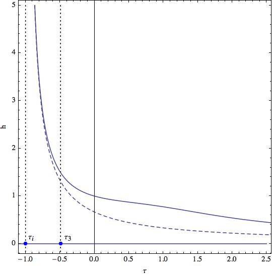
Figure 1: A typical example of the expansion rate or ${\cal H}$ as a function of time $\tau$ for $t_{U}\simeq 13.9$ Gyears (this is for $\tau_{i}\simeq-1)$ and $w_{0}\simeq-0.962$. The dashed curve represents the usual $\frac{2}{3}/(\tau-\tau_{i})$ law of standard FRW$\Lambda$ cosmology. The asymptotic continuations follow the laws given in (1.11). The vertical doted lines are at $\tau_{i}\simeq-1$ and $\tau_{3}\simeq-0.5.$

An example of $\Omega_{\Lambda}$ as a function of $\tau$ is shown in figure 2. Notice that $\Omega_{\Lambda}\simeq{\Omega_{\Lambda}}_{c}>{\Omega_{\Lambda}}_{0}$, for $\tau\leq\tau_{3}$. For $\tau>\tau_{3}$, $\Omega_{\Lambda}$ decreases going down to zero at future infinity.

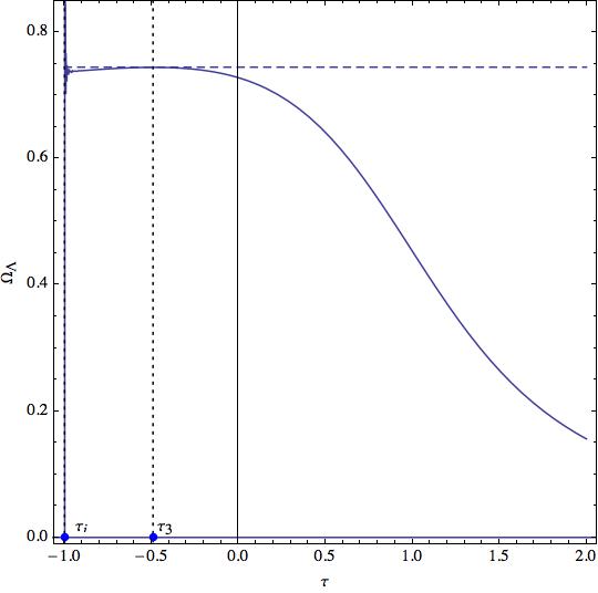
Figure 2: A typical example for $\Omega_{\Lambda}$ as a function of $\tau$ for $t_{U}\simeq 13.9$ Gyears and $w_{0}\simeq-0.962$. The dashed horizontal line is $\Omega_{\Lambda}={\Omega_{\Lambda}}_{c}$ The asymptotic continuations for $\tau\rightarrow\infty$ is $\Omega_{\Lambda}\rightarrow 1/(3K_{+}\tau^{2})\simeq 0.718/\tau^{2}$. Notice the oscillations of $\Omega_{\Lambda}$ where $\tau\rightarrow\tau_{i}$. This is a Mathematica feature due to the fact that $\Omega_{\Lambda}$ is equal to a difference of two quantities both of which become equal but infinite. Perhaps ${\Omega_{\Lambda}}_{i}\rightarrow 0$ brutally.

Perhaps the most interesting feature of the model is that reasonable configurations, that is for $\rho\geq 0$, exist only for a limited range of values of $w_{0}$ which depends on $t_{U}$ as shown in Figure 3:

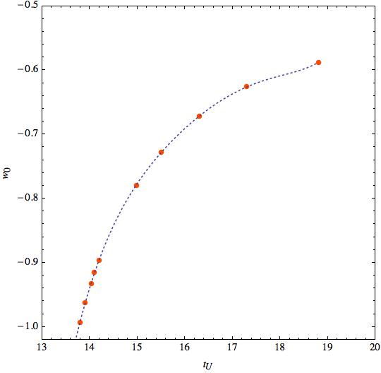
Figure 3: The time derivative today ${\Omega_{\Lambda}}^{\prime}_{0}$ or rather its associated parameter $w_{0}$ as a function of the age of the universe $t_{U}$ in Gyears. Present day measurement is about the last point on the bottom left. The continuous dotted line is a polynomial fit of order $5$.

$$~{}~{}~{}~{}13.8\lesssim t_{U}\lesssim 29.5~{}~{}~{}~{},~{}~{}~{}-0.993\lesssim w_{0}\lesssim-0.535.$$

Accordingly at present, with $t_{U0}\simeq 13.75$ Gyears the prediction is $w_{0}\simeq-0.99$.

(i) Problems with the model

One problem is that $c_{1}(\tau_{2})$ and $c_{2}(\tau_{2})$ go to zero at $\tau_{1}<\tau_{i}$ as can be seen in Figure 4.

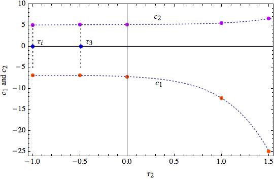
Figure 4: $c_{1}$ and $c_{2}$ as functions of $\tau_{2}$. The dotted lines are polynomial fittings of order $5$.

Unfortunately, Mathematica cannot reach beyond the singularity. This may not be a serious flaw from a physical point of view. Given $\tau_{1}$ and $h(\tau_{1})$, equation (1.5) has smooth numerical solutions. However, none were found with the energy density $\rho$ always positive. Another problem is that equations (1.2) are no more Einstein’s equations. It is plausible that Einstein’s equations with their purely local conservation of the matter energy momentum tensor are not valid at cosmological scales.

(iii) Conclusion

Equations (1.2) are in some respects appealing. Results are surprisingly close to observations with such a primitive model. No adjustable parameters, no scalar fields coming from nowhere, no “quintessence”. The cosmological “constant” varies mildly, is positive and remains small. Both $\Omega_{\Lambda}$ and $\Omega_{m}$ become and stay of the same order of magnitude at any later time and tend to zero in the future. The coincidence problem is far less acute. The model predicts a relation between $w_{0}$ and $t_{U0}$ which is remarkably close to observations. For those reasons, the present unusual variational principle deserved some attention.

Finally a referee of the editorial board brought to our attention a paper by Kaloper and Padilla [3] whose motivations are light years away from ours but whose starting point involves as here the 4-volume of spacetime time to remove the disturbing effect of the vacuum energy on the cosmological constant. The authors need a finite space which leads inevitably to a final crunch. We took spacetime to be flat for simplicity. A closed spacetime would certainly be more in tune with Mach’s principles.

Acknowledgments

I thank Nathalie Deruelle for her insight into the properties of equation (1.7) which is much appreciated. I also thank Donald Lynden-Bell for his enthusiasm with the differential equations which was illuminating in many ways and very helpful.

References

- [1] Bronstein M 1933 On the expanding universe Phys. Z. Sowjetunion 3 73
- [2] Davidson A and Rubin S 2009 Zero cosmological constant from normalised general relativity Class. Quantum Grav. 26 235019 (Preprint: arXiv:gr/qc 0905.0661)
- [3] Kaloper N and Padilla W 2013 Sequestering the standard model vacuum energy Preprint: arXiv:1309.6562v1 [hep-ph] 25 September 2013
- [4] Komatsu et al 2011 Seven year Wilkinson Microwave Anisotropy Probe (WMAP) observations: cosmological interpretation ApJS 192 18
- [5] Larson et al 2011 Seven year Wilkinson Microwave Anisotropy Probe (WMAP) observations: power spectra and WMAP-derived parameters ApJS 192 16
- [6] Lynden Bell D 2010 Searching for insight Annu. Rev. Astro. Astrophys. 48 1 (see p. 6)
- [7] Peebles P J E and Ratra B 2003 The cosmological constant and dark energy Rev. Mod. Phys. 75 559
- [8] Planck Collaboration 2013 Planck 2013 results. XVI. Cosmological parameters A & A Submitted, Preprint: arXiv:1303.5076v1 [astro-ph.CO] 20 Mars 2013
- [9] Riess et al 2011 A 3% solution: Determination of the Hubble Constant with the Hubble Space Telescope and wide field camera 3 ApJ 730 119
- [10] Schutz B F and Sorkin R 1077 Variational aspects of relativistic field theories, with applications to perfect fluids Ann. of Phys. 107 1
- [11] Tseytlin A A 1991 Duality-symmetric string theory and the cosmological-constant problem Phys. Rev. L. 66 545