Oblique propagation of dust ion-acoustic solitary waves in a magnetized dusty pair-ion plasma

Abstract

We investigate the propagation characteristics of electrostatic waves in a magnetized pair-ion plasma with immobile charged dusts. It is shown that obliquely propagating (OP) low-frequency (in comparison with the negative-ion cyclotron frequency) long-wavelength “slow” and “fast” modes can propagate, respectively, as dust ion-acoustic (DIA) and dust ion-cyclotron (DIC)-like waves. The properties of these modes are studied with the effects of obliqueness of propagation $(\theta)$, the static magnetic field, the ratios of the negative to positive ion masses $(m)$ and temperatures $(T)$ as well as the dust to negative-ion number density ratio $(\delta)$. Using the standard reductive perturbation technique, we derive a Korteweg-de Vries (KdV) equation which governs the evolution of small-amplitude OP DIA waves. It is found that the KdV equation admits only rarefactive solitons in plasmas with $m$ well below its critical value $m_{c}~{}(\gg 1)$ which typically depends on $T$ and $\delta$. It is shown that the nonlinear coefficient of the KdV equation vanishes at $m=m_{c}$, i.e., for plasmas with much heavier negative ions, and the evolution of the DIA waves is then described by a modified KdV (mKdV) equation. The latter is shown to have only compressive soliton solution. The properties of both the KdV and mKdV solitons are studied with the system parameters as above, and possible applications of our results to laboratory and space plasmas are briefly discussed.

I Introduction

Typical plasmas consisting of electrons and ions or similar particles with large-mass difference essentially cause temporal as well as spatial variations of collective plasma phenomena. However, the space-time parity can be maintained in pair-ion plasmas with equal mass or a slightly different masses. Plasmas containing positive and negative ions not only found in naturally occurring plasmas, but are also used for technological applications. In many industries, e.g., in integrated-circuit fabrication, since the deposited film is strongly damaged by a high-energy electron, a plasma source having no energetic electrons is required. For this purpose, a radio-frequency plasma source has also been developed yabe1994 . Pure pair-ion plasmas with equal mass and temperature have been generated in the laboratory, and three kinds of electrostatic modes, namely the ion-acoustic wave (IAW), the intermediate-frequency wave (IFW), and the ion plasma wave (IPW), have been experimentally observed using fullerene as an ion source pair-ion-experiment . Later, a criterion for the description of pure pair-ion plasmas has been investigated by Saleem saleem-pair-ion . Recently, there has been a growing interest in investigating the properties of electrostatic waves in pair-ion plasmas in linear and nonlinear regimes (See, e.g., pair-ion1 ; pair-ion2 ; pair-ion3 ; pair-ion4 ; pair-ion5 ; pair-ion-charging-theory ; pair-ion-charging-experiment ; pair-ion-instability ). To mention few, Misra et al. pair-ion1 had investigated the propagation of dust ion-acoustic (DIA) solitary waves and shocks (SWS) in an unmagnetized dusty negative-ion plasma. They found that the SWS exist with negative potential when dusts are positively charged. Rosenberg and Merlino pair-ion-instability studied the ion-acoustic instability in a dusty negative-ion plasma. The theory of dust-acoustic solitons in unmagnetized pair-ion-electron plasmas has been investigated through the description of Korteweg-de Vries (KdV) equation pair-ion2 . More recently, the linear and nonlinear properties of both small- and large-amplitude DIA solitary waves in an unmagnetized pair-ion plasma with immobile charged dusts have been studied pair-ion5 . It has been shown that pair-ion plasmas with positively charged dusts support DIA solitons only of the rarefactive type. There are, however, a number of recent works dealing with the nonlinear properties of solitary waves solitary-sultana ; williams2013 ; sultana2010 ; mamun2002 ; kourakis2004a ; kourakis2004b ; paul2013 ; mamun1998 ; saini2008 ; bandyopadhyay1999 , electrostatic ion-cyclotron waves ion-cyclotron-shukla shocks shocks1 in other plasma environments.

The presence of negative ions in the Earth’s D and lower E regions at altitudes about $73-90$ km narcisi1971 as well as in Titan’s atmosphere coates2007 have been detected. These negative ions act as a precursors for the formation of massive charged dust particles, which, e.g., in a processing reactor can contaminate the product choi1993 . The in situ measurements of charged particles in the polar mesosphere under nighttime conditions revealed the existence of positively charged dusts which are dominated by both positive and negative ions, and few percentage of electrons in-situ-Rapp . Also, it has been shown that such positively charged dust particles are due to the presence of sufficiently heavy and numerous negative ions (i.e., $m_{n}>300$ amu and $n_{n0}\gtrsim 50n_{e0}$, where $m_{n}$ is the negative-ion mass, and $n_{e0}$, $n_{n0}$ are, respectively, the number densities of electrons and negative ions) in-situ-Rapp . Furthermore, it has been observed that the dust particles injected into a pair-ion plasma (e.g., $K^{+}/SF_{6}^{-}$ plasmas) can become positively charged when $n_{n0}\gtrsim 500n_{e0}$ pair-ion-charging-experiment ; pair-ion-charging-theory . On the other hand, there has been a number of observations to detect solitary structures in space plasma environments. To mention few, the Viking spacecraft and Freja satellite have indicated the presence of electrostatic solitary structures in the Earth’s magnetosphere dovner1994 . Williams et al. williams2006 have reported the observations of solitary waves by the Cassini spacecraft in the vicinity of Saturn’s magnetosphere (with ambient magnetic fields $\sim 0.1-8000$ nT). It has also been suggested that the turbulence in Earth’s magnetosheath may account for the observations of many solitary pulses observed there pickett2004 . It is thus of great interest and importance to extend the theory of ion waves pair-ion-experiment ; pair-ion-charging-experiment in magnetized pair-ion plasmas with a background of positively charged dusts.

In this wok, we consider a dusty pair-ion plasma in presence of an external magnetic field, and use a three-dimensional fluid model for the propagation of DIA waves obliquely to the magnetic field. We show that apart from the usual DIA and dust ion-cyclotron (DIC) modes, which appear for wave propagation parallel and perpendicular to the magnetic field, there also exist obliquely propagating very low-frequency (compared to the negative-ion cyclotron frequency) long-wavelength fast and slow modes, which are similar to DIC and DIA waves. Using the standard reductive perturbation technique, we derive KdV and modified KdV (mKdV) equations to describe the evolution of nonlinear DIA waves in plasmas with $m<m_{c}$ and $m\sim m_{c}$ respectively, where $m$ is the mass ratio between negative and positive ions and $m_{c}$ is its critical value. It is shown that the KdV and mKdV equations admit rarefactive and compressive solitons in plasmas with $m>1$ and $m\gg 1$ respectively.

II Basic Equations

We consider the propagation of electrostatic waves in a magnetized collisionless dusty plasma consisting of singly charged adiabatic positive and negative ions, and positively charged dusts. The latter are assumed to be of uniform size and immobile, since we are concerned with the occurrence of DIA and DIC waves, whose phase speeds are much larger than the ion- and dust-thermal speeds, on a time scale much shorter than the dust plasma and dust gyroperiods. Thus, the charged dust grains do not have time to respond to the DIA and DIC oscillations, and subsequently there are insignificant dust number density perturbations. However, the effects of the positively charged dusts then appear through the modification of the charge neutrality condition:

$$n_{p0}+z_{d}n_{d0}=n_{n0},$$ (1)

where $n_{j0}$ is the unperturbed number density of species $j$ ($j$=$p$, $n$, $d$, respectively, stand for positive ions, negative ions, and static charged dusts), $z_{d}$ $(>0)$ is the unperturbed dust charge state.

We consider a hydrodynamic model in which the negative ion fluids are heavier than the positive ions, and negative ion number density is much larger than that of electrons so that dusts become positively charged pair-ion-charging-experiment ; pair-ion1 ; pair-ion5 . Thus, the dominant higher mobility species in the plasma are the positive ions. In DIA and DIC waves, since the thermal motion of ions can not keep up with the wave, both positive and negative ions are adiabatically compressed, and we assume the adiabatic compression of the ion fluids pair-ion1 ; pair-ion5 . Furthermore, since the negative ion number density is larger than that of the positive ions [Eq. (1)] in presence of positively charged dusts, the phase speed of the DIA wave is somewhat enhanced in comparison with that of the ion-acoustic waves in pair-ion plasmas without charged dusts. The wave propagation is considered in an arbitrary direction with respect to the static magnetic filed $\mathbf{B}=B_{0}\hat{z}$, and ions are magnetized.

The basic equations for the dynamics of positive and negative ions in presence of the static magnetic field are

$$\frac{\partial n_{j}}{\partial t}+\nabla\cdot(n_{j}\mathbf{v}_{j})=0,$$ (2)

$$\frac{d\mathbf{v}_{j}}{dt}=\frac{q_{j}}{m_{j}}\left(\mathbf{E}+\mathbf{v}_{j}\times\frac{1}{c}B_{0}\hat{z}\right)-\frac{\nabla P_{j}}{m_{j}n_{j}},$$ (3)

$$\nabla\cdot\mathbf{E}=4\pi e(n_{p}-n_{n}+z_{d}n_{d0}),$$ (4)

where $d\mathbf{v}_{j}/dt\equiv\partial/\partial t+\mathbf{v}_{j}\cdot\nabla$, and $n_{j}$, $\mathbf{v}_{j}$, and $m_{j}$, respectively, denote the number density, velocity, and mass of $j$-species particles [$j=p(n)$ stands for positive (negative) ions]. Also, $q_{p}=e$, $q_{n}=-e$, $e(>0)$ being the elementary charge, and $\mathbf{E}=-\nabla\phi$ with $\phi$ denoting the electrostatic potential.

Equations (2) to (4) can be recast in terms of dimensionless variables. Thus, we normalize the physical quantities according to $\phi\rightarrow e\phi/k_{B}T_{p}$, $n_{j}\rightarrow n_{j}/n_{j0}$, $v_{j}\rightarrow v_{j}/c_{s}$, where $c_{s}=\sqrt{k_{B}T_{p}/m_{n}}=\omega_{pn}\lambda_{D}$ is the ion-acoustic speed with $\omega_{pn}=\sqrt{4\pi n_{n0}e^{2}/m_{n}}$ and $\lambda_{D}=\sqrt{k_{B}T_{p}/4\pi n_{n0}e^{2}}$ denoting, respectively, the negative-ion plasma frequency and the plasma Debye length. Here, $T_{j}$ is the thermodynamic temperature of j-species ions and $k_{B}$ is the Boltzmann constant. The space and time variables are normalized by $\lambda_{D}$ and $\omega^{-1}_{pn}$ respectively. In Eq. (3), we consider the adiabatic pressure law as pair-ion1 ; pair-ion5 $P_{j}/P_{j0}=(n_{j}/n_{j0})^{\gamma}$ with $P_{j0}=n_{j0}k_{B}T_{j}$ for each ion-species $(j=p,n)$, and the adiabatic index $\gamma=5/3$ $[=(2+D)/D$, $D$ being the number of degrees of freedom]. It is to be mentioned that in the propagation of very low-frequency waves (in comparison with the negative-ion cyclotron frequency), the phase speed $v_{p}$ of the DIA waves is to be much higher than the thermal speed $v_{tn}$ of negative ions as well as much lower than the positive-ion thermal speed $v_{tp}$, i.e., $v_{tn}\ll v_{p}\ll v_{tp}$, in order to avoid the wave damping due to the resonance with positive or negative ions. This feature can be verified from the linear dispersion relation to be obtained in the next section.
Thus, from Eqs. (2) to (4), we obtain the following set of equations in dimensionless form:

$$\frac{\partial n_{j}}{\partial t}+\nabla\cdot(n_{j}\mathbf{v}_{j})=0,$$ (5)

$$\frac{d\mathbf{v}_{j}}{dt}= -\zeta_{j}\left(\frac{m_{n}}{m_{j}}\nabla\phi-\mathbf{v}_{j}\times\omega_{cj}\hat{z}\right)$$ (6)

$$-\frac{5}{3}\frac{m_{n}T_{j}}{m_{j}T_{p}}n^{-{1/3}}_{p}\nabla n_{j},$$

$$\nabla^{2}\phi=n_{n}-\mu n_{p}-\delta,$$ (7)

together with the charge neutrality condition given by

$$\mu+\delta=1,$$ (8)

where $\zeta_{p}=1$, $\zeta_{n}=-1$, $\omega_{cj}=eB_{0}/cm_{j}\omega_{pn}$ is the cyclotron frequency for the $j$-th species of ions, normalized by the negative-ion plasma frequency, $\mu=n_{p0}/n_{n0}$, and $\delta=z_{d}n_{d0}/n_{n0}$.

III Dispersion relation: Linear waves

In the linearization process (very small-amplitude limit), we split-up the physical quantities into its unperturbed and perturbed parts according to $n_{j}=1+n_{j1}$, $\mathbf{v}_{j}=\mathbf{v}_{j1}$, $\phi=\phi_{1}$. The perturbations are then considered to vary as $\varpropto\exp(i\mathbf{k}\cdot\mathbf{r}-i\omega t)$, i.e., in the form of oscillations with wave frequency $\omega$ and wave number $k$. Thus, Fourier analyzing Eqs. (5)-(7) we obtain (omitting the subscripts $1$)

$$-\omega n_{j}+\mathbf{k}\cdot\mathbf{v}_{j}=0,$$ (9)

$$-\omega\mathbf{v}_{p}+i\left(\mathbf{v}_{p}\times\omega_{cp}\hat{z}\right)+m\mathbf{k}\left(\phi+\frac{5}{3}n_{p}\right)=0,$$ (10)

$$-\omega\mathbf{v}_{n}-i\left(\mathbf{v}_{n}\times\omega_{cn}\hat{z}\right)+\mathbf{k}\left(-\phi+\frac{5}{3}Tn_{n}\right)=0,$$ (11)

$$n_{n}-\mu n_{p}+k^{2}\phi=0,$$ (12)

where we denote $m=m_{n}/m_{p}$ and $T=T_{n}/T_{p}$ as the mass and temperature ratios of negative to positive ions. Taking dot product of Eq. (10) with $\mathbf{k}$, and using Eq. (9) we obtain

$$n_{p}\left(-\omega^{2}+\frac{5}{3}mk^{2}\right)+mk^{2}\phi+i\omega_{cp}\left(k_{x}v_{py}-k_{y}v_{px}\right)=0,$$ (13)

From the $x$- and $y$-components of Eq. (10), we solve for $v_{px}$ and $v_{py}$ to yield the following expressions

$$v_{px}=m\left[\frac{\omega k_{x}+i\omega_{cp}k_{y}}{\omega^{2}-\omega^{2}_{cp}}\right]\left(\phi+\frac{5}{3}n_{p}\right),$$ (14)

$$v_{py}=m\left[\frac{\omega k_{y}-i\omega_{cp}k_{x}}{\omega^{2}-\omega^{2}_{cp}}\right]\left(\phi+\frac{5}{3}n_{p}\right).$$ (15)

Substituting the expressions from Eqs. (14) and (15) into Eq. (13), we obtain the following expression for the perturbed number density of positive ions

$$n_{p}=\frac{mA_{p}}{B_{p}}\phi,$$ (16)

where $A_{p}$ and $B_{p}$ are given by

$$A_{p}=\omega^{2}k^{2}-\omega^{2}_{cp}k^{2}_{z},$$ (17)

$$B_{p}=\omega^{2}\left(\omega^{2}-\frac{5}{3}mk^{2}\right)-\omega^{2}_{cp}\left(\omega^{2}-\frac{5}{3}mk_{z}^{2}\right).$$ (18)

Proceeding in the same way as for $n_{p}$ of positive ions, we obtain from Eqs. (9) and (11) the similar expression for the negative ions as

$$n_{n}=-\frac{A_{n}}{B_{n}}\phi,$$ (19)

where $A_{n}$ and $B_{n}$ are given by

$$A_{n}=\omega^{2}k^{2}-\omega^{2}_{cn}k^{2}_{z},$$ (20)

$$B_{n}=\omega^{2}\left(\omega^{2}-\frac{5}{3}Tk^{2}\right)-\omega^{2}_{cn}\left(\omega^{2}-\frac{5}{3}Tk_{z}^{2}\right).$$ (21)

Next, substituting the expressions for $n_{n}$ and $n_{p}$ from Eqs. (16) and (19) into Eq. (12), and assuming that the perturbation $\phi$ is nonzero, we obtain the following linear dispersion relation:

$$\sum_{j=p,n}{\frac{\left(m_{n}n_{j0}/m_{j}n_{n0}\right)f_{cj}}{\omega^{2}\left(1-g_{cj}\right)-5k_{z}^{2}v^{2}_{tj}/3}}=1,$$ (22)

where $f_{cj}=k^{2}_{z}/k^{2}-\omega^{2}/\omega^{2}_{cj}$ and $g_{cj}=\left(\omega^{2}-{5}k^{2}v^{2}_{tj}/3\right)/\omega^{2}_{cj}$ in which $v_{tj}=\sqrt{k_{B}T_{j}/m_{j}}/c_{s}$ is the thermal velocity for $j$-species of ions, normalized by $c_{s}$. Note, however, that the second term of $f_{cj}$, and $g_{cj}$ appear due to the effects of the static magnetic field and the velocity perturbations transverse to it. By disregarding these effects, and considering one-dimensional wave propagation (Hence replacing the factor $5/3$ by $3$ as the contribution from the thermal adiabatic pressure in one-dimensional propagation), one can recover the dispersion relation for dust ion-acoustic waves in unmagnetized plasmas (See Eq. (9) of Ref. pair-ion5 ). The dispersion relation (22) thus generalizes and extends the work of Ref. pair-ion5 to provide some new wave modes that were not reported before. From this dispersion relation, we not only recover the usual DIA and DIC modes, but also some other low-frequency (compared to the negative-ion cyclotron frequency) long-wavelength DIA and DIC-like modes. On the left-side of Eq. (22), the first (second) term is the contribution from positive (negative) ion fluids whose equilibrium are under the electrostatic force, the Lorentz force, and the adiabatic pressure, whereas the nonzero value $1$ on the right-hand side is from the higher-order dispersive effects due to separation of charged particles (Deviation from quasi-neutrality in the perturbed state). From the dispersion relation (22) we find, in particular, that in order to avoid the wave damping for very low-frequency waves ($\omega^{2}\ll\omega^{2}_{cn}\ll\omega^{2}_{cp}$ with $g_{cj}\ll 1$) due to the resonance with either the positive or negative ions, the phase speed of the wave is to be much higher than the negative-ion thermal speed $v_{tn}$ and much lower than the positive-ion thermal speed $v_{tp}$. Such wave damping may arise in an unmagnetized pair-ion plasma pair-ion5 or plasmas with one group of ions ppcf-sultana . The dispersion equation (22) is of degree eight in $\omega$, and, in general, can give eight wave modes. However, we will be interested to study the properties of some useful wave modes as mentioned above at some interesting limiting cases as discussed below.

First of all, in the quasineutrality limit (valid for long-wavelength modes) and in the low-frequency approximation, i.e., $\omega^{2}\ll\omega^{2}_{cn}\ll\omega^{2}_{cp}$, we obtain from Eq. (22) the following wave modes

$$\omega^{2}\approx\frac{1}{2}\left(\frac{m\mu}{\omega^{2}_{cp}}+\frac{1}{\omega^{2}_{cn}}\right)^{-1}\left[\alpha_{1}+\alpha_{2}k^{2}\pm\sqrt{\left(\alpha_{1}-\alpha_{2}k^{2}\right)^{2}+\frac{20}{3}m\mu(m-T)\left(\frac{1}{\omega^{2}_{cn}}-\frac{1}{\omega^{2}_{cp}}\right)k^{2}\cos^{2}\theta}\right],$$ (23)

where

$$\alpha_{1}=\left(1+m\mu\right)\cos^{2}\theta,\hskip 5.0pt\alpha_{2}=\frac{5}{3}m\left(\frac{\mu T}{\omega^{2}_{cp}}+\frac{1}{\omega^{2}_{cn}}\right),$$ (24)

and ${k_{z}}={k}\cos\theta$, $\theta$ being the angle between the magnetic field and the wave vector. The upper (plus) and lower (minus) signs in Eq. (23) represent, respectively, the electrostatic low-frequency fast and slow waves which propagate obliquely to the external magnetic field. The phase velocities of these waves approach a maximum value in the long-wavelength limits.

Figure 1 shows the characteristics of the low-frequency fast and slow modes [Eq. (23)] by the effects of (i) the obliqueness of wave propagation $(\theta)$, (ii) the static magnetic field $(\omega_{cp})$, (iii) the negative to positive-ion mass ratio $(m)$, (iv) the immobile positively charged dusts $(\delta)$ and (v) the negative to positive ion temperature ratio $(T)$. We find that the obliquely propagating slow (lower branch) and fast modes (upper branch) correspond, respectively, to the DIA and DIC-like waves. Below we discuss the properties of these modes separately.

(i) Effect of oblique wave propagation: The effect of the propagation angle $\theta$ on the linear properties of the low-frequency modes are shown in Fig. 1. It is found that increasing the angle with respect to the magnetic field leads to a decrease in the frequency $\omega$ of both the fast (upper branch) and slow (lower branch) modes along with the modification of their phase speeds. Furthermore, the effect of $\theta$ on the fast mode is significant for $k\rightarrow 0$, while its effect on the slow mode is noticeable for $k\gtrsim 0.03$. It is also seen that the frequency gap between the modes decreases with increasing the angle $\theta$. An opposite trend of increasing the frequency gap by the effect of $\theta$ was found for oblique electron-acoustic waves in a magnetized kappa-distributed electron-ion plasma ppcf-sultana .

(ii) Magnetic field effect: The influence of the magnetic field strength (characterized by $\omega_{cj},~{}j=p,n$) on the wave modes is shown in Fig. 1. Both the weaker $(\omega_{cj}<1)$ and the stronger $(\omega_{cj}>1)$ magnetic fields increase the frequency gap between the modes. However, a significant increase in the frequency of the DIC waves (upper branch), and hence a significant increase of the frequency gap between the modes, is seen to occur for stronger magnetic fields. It is also found that the phase speed of the DIA modes remain constant as $k\rightarrow 0$. These interesting features of DIA and DIC-like modes have not been observed before in pair-ion plasmas pair-ion1 ; pair-ion2 ; pair-ion3 ; pair-ion4 ; pair-ion5

(iii) Effect of negative to positive ion mass ratio: The effects of the mass ratio $m$ on the fast or DIC (upper branch) and slow or DIA (lower branch) modes are shown in Fig. 1. Interestingly, as $m$ increases, i.e., as the mass difference between the ions increases, the wave frequency of the fast mode increases for a wave number exceeding a critical value (This value is different for different values of $m$), otherwise it decreases as $k\rightarrow 0$. On the other hand, the mass ratio $m$ has almost the similar influence on the slow modes as in Fig. 1 (lower curves).

(iv) Effect of immobile charged dusts: Figure 1 shows the effect of the presence of positively charged dusts in the background plasma. It is found that increasing the concentration of charged dusts $\delta$ (hence decreasing the positive- to negative-ion density ratio $\mu$ to maintain the charge neutrality) leads to an increase in the frequency $\omega$ of the upper mode (DIC), and a frequency decrease in the lower DIA mode. This occurs when the wave number exceeds its critical value $k_{c}$ lying in $0.2<k<0.3$. However, for $k<k_{c}$, the opposite trend occurs for both the modes along with the modification of their phase speeds. As a result, the frequency gap between the modes for $k>k_{c}$ $(k<k_{c})$ is found to increase (decrease). Thus, the presence of immobile charged dusts not only modifies the wave frequency and the phase speed, but also reduces the frequency gap between the DIA and DIC-like modes, which can not be observed in pure pair-ion plasmas with equal mass and temperature pair-ion-experiment ; saleem-pair-ion ; pair-ion2 ; pair-ion3 . However, some different features of increasing the frequency gap (not the decreasing trend) between DIA and DIC modes were found, e.g., for oblique propagation of electron-acoustic waves in a magnetized plasma without charged dusts ppcf-sultana .

(v) Effect of negative to positive ion temperature ratio: The effects of the thermal pressures of ions on both the fast (upper branch) and slow (lower branch) modes are exhibited in Fig. 1. It is seen that the temperature ratio $T$ of negative to positive ions has stronger influence with increasing the frequency of the DIA mode (lower branch) than the DIC (upper branch) mode. In the latter, the change of wave frequency with $T$ is noticeable for wave numbers satisfying $k\gtrsim 0.25$. Furthermore, as in Fig. 1, the increase (decrease) of the frequency gap between the modes at short (long)-wavelengths is seen to occur.

From the results (iii) and (v), one may thus conclude that the properties of the DIA and DIC modes in pair-ion plasmas with different mass and temperatures of ions are quite distinctive to those found in pair-ion plasmas with equal mass and temperature of ions pair-ion-experiment ; saleem-pair-ion ; pair-ion2 ; pair-ion3 .

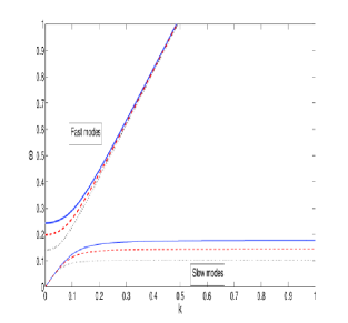
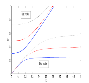
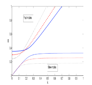
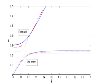
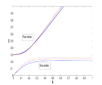
Figure 1: Effects of (a) the obliqueness of propagation $(l_{z})$, (b) the external magnetic field $(\omega_{cp})$, (c) the ratio of negative and positive ion masses $(m)$ (d) positively charged dusts $(\delta)$ and (e) the negative to positive ion temperature ratio $(T)$ on the low-frequency modes given by Eq. (23) are shown. In each subfigure, the upper (three thick lines) and the lower (three thin lines) curves, respectively, correspond to the fast (DIC-like) and slow (DIA) modes. Subfigure (a): Different values of the propagation angle $\theta$ are $\theta=\pi/6$ (solid line), $\pi/4$ (dashed line), and $\pi/3$ (dotted line); the fixed parameter values are $T=0.7,~{}\delta=0.1,~{}m=3$, and $\omega_{cp}=0.5$. Subfigure (b): Different values of $\omega_{cp}$ are $\omega_{cp}=0.5$ (solid line), $\omega_{cp}=0.8$ (dashed line), and $\omega_{cp}=1.2$ (dotted line); the fixed parameter values are $T=0.5,~{}m=2$, $\theta=\pi/6$ and $\delta=0.1$. Subfigure (c): Different values of $m$ are $m=1.5$ (solid line), $m=2.0$ (dashed line), and $m=3$ (dotted line); the fixed parameter values are $T=0.7$, $\delta=0.1$, $\theta=\pi/6$ and $\omega_{cp}=0.5$. Subfigure (d): Different values of $\delta$ are $\delta=0.05$ (solid line), $\delta=0.5$ (dashed line), and $\delta=0.9$ (dotted line); the fixed parameter values are $T=0.5,~{}m=2$, $\theta=\pi/6$ and $\omega_{cp}=0.5$. Subfigure (e): Different values of $T$ are $T=0.1$ (solid line), $T=0.5$ (dashed line), and $T=0.9$ (dotted line); the fixed parameter values are $m=2$, $\delta=0.1$, $\theta=\pi/6$ and $\omega_{cp}=0.5$.

Secondly, for wave propagation along the magnetic filed we have $k_{x}$, $k_{y}\longrightarrow 0$; $k_{z}=k_{\parallel}\neq 0$. In this case, the transverse velocity components of the ion fluids vanish [See Eqs. (14), (15) and similar equations for negative ions, not shown], and particles will have velocities only along the magnetic field. Thus, we have electrostatic DIA wave modes, the dispersion relation of which is obtained from Eq. (22) as

$$\omega^{2}=\frac{1}{2}\left[1+m\mu+\frac{5}{3}(m+T)k^{2}_{\parallel}\pm\sqrt{\left(m\mu-1+\frac{5}{3}(m-T)k^{2}_{\parallel}\right)^{2}+4m\mu}\right].$$ (25)

The upper and lower signs in Eq. (25), respectively, correspond to the fast and slow DIA modes that are modified by the different mass and temperatures of ions as well as the presence of positively charged dusts. In particular, for plasmas with equal mass and temperature of ions, i.e., $m=T=1$, and with no dust, i.e., $\mu=1$, the slow wave becomes dispersionless with a phase speed independent of the wave number $k$, while the fast mode propagates similar to the high-frequency (in comparison with the plasma oscillation frequency) electron-acoustic waves in an unmagnetized electron-ion plasma. In the quasineutrality limit (valid for long-wavelength modes), Eq. (22) reduces to

$$\omega=k_{\parallel}\sqrt{\frac{5}{3}m\left(\frac{1+T\mu}{1+m\mu}\right)}.$$ (26)

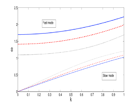
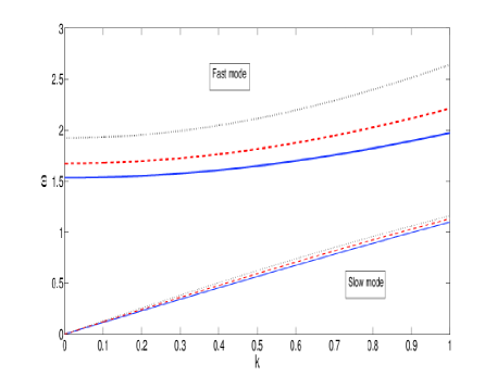
Figure 2: Effects of (a) positively charged dusts $(\delta)$ and (b) the ratio of negative and positive ion masses $(m)$ on the DIA modes given by Eq. (25) are shown. In each subfigure, the upper (three thick lines) and the lower (three thin lines) curves, respectively, correspond to the fast and slow DIA modes. For the subfigures (a) and (b), different values of the parameters $\delta$ and $m$, as well as the corresponding fixed parameter values are considered as the same as in Figs. 1 and 1 respectively.

From Eqs. (25) and (26), we find that the electrostatic waves, while propagating parallel to the static magnetic field, are purely longitudinal acoustic-like waves (similar to the case of no magnetic field) with its frequency being independent of the magnetic field, and they are dispersive due to the effects of charge separation (deviation from quasineutrality) of the ion fluids. The phase velocities of these waves increase with the wave number and are greater than the acoustic speed for the ion fluids. Furthermore, these waves become dispersionless in the long-wavelength limits, and propagate with a constant phase speed.

It may be instructive to analyze the properties of the DIA modes [Eq. (25)], which typically depend on the plasma parameters, namely $\delta,~{}T$ and $m$. The features are shown in Fig. 2. Figure 2 shows that as the charged dust concentration increases (i.e., the positive to negative ion density ratio decreases), the frequency of the slow mode (lower branch) increases, while for the fast modes it decreases significantly. Furthermore, increasing the dust density leads to reducing the frequency gap between the modes. It is also seen that the effect of $\delta$ is significant for both the short and long-wavelength fast modes, while its effect on the long-wavelength slow modes is comparatively weak. In contrast to the properties of the fast modes in Fig. 2 with the effect of $\delta$, Fig. 2 shows that as the mass ratio $m$ increases, the frequencies of both the fast and slow modes increase along with the increase in the frequency gap between the modes. It is evident from Eq. (26) and from the lower branches of Fig. 2 that the phase velocity of the DIA mode remains constant as $k\rightarrow 0$, i.e., in the long-wavelength limit. Furthermore, it is found that (not shown in the figure) the effect of the temperature ratio $T$ on the fast DIA modes is almost negligible, while it increases the frequency of the slow modes similar to that observed in Fig. 2.

Lastly, we consider the wave propagation perpendicular to the magnetic filed, i.e., propagation for $k_{z}\longrightarrow 0$, $k^{2}_{x}+k^{2}_{y}=k^{2}_{\perp}\neq 0$. In this case, ions have velocity components only transverse to the magnetic field. The dispersion Eq. (22) then reduces to

$$\omega^{2}=\frac{1}{2}\left[1+m\mu+\omega^{2}_{cp}+\omega^{2}_{cn}+\frac{5}{3}(m+T)k^{2}_{\perp}\pm\sqrt{\left(m\mu-1+\omega^{2}_{cp}-\omega^{2}_{cn}+\frac{5}{3}(m-T)k^{2}_{\perp}\right)^{2}+4m\mu}\right].$$ (27)

This represents a DIC wave modified by the effects of the external magnetic field, different mass and temperature of the ion fluids as well the presence of static charged dusts. Note that in the limit of vanishing-magnetic field, Eq. (27) trivially recovers the same form as Eq. (25) for modified DIA waves. In the quasineutrality limit, Eq. (27) reduces to the following DIC mode

$$\omega^{2}=\frac{\omega^{2}_{cp}+m\mu\omega^{2}_{cn}}{1+m\mu}+{\frac{5}{3}m\left(\frac{1+T\mu}{1+m\mu}\right)k^{2}_{\perp}}.$$ (28)

In particular, for $m=T=1$ and $\omega_{cp}=\omega_{cn}=\omega_{c}$, we recover from Eq. (28) the following ion-cyclotron mode similar to that appears in magnetized electron-ion plasmas with Boltzmann distributed electrons:

$$\omega^{2}=\omega_{c}^{2}+\frac{5}{3}k^{2}_{\perp}.$$ (29)

The factor $5/3$ appears due to the adiabatic pressure of ion fluids in three-dimensional configuration.

The properties of the DIC modes given by Eq. (27) are shown in Fig. 3 for a set of parameters as in Fig. 1. It is found that in contrast to the features of the slow mode (lower branch), as $\delta$ increases or the density ratio $\mu$ decreases to maintain the quasineutrality, the frequency of the DIC mode decreases significantly [See Fig. 3]. The influence of the magnetic field (represented by $\omega_{cj}$) is depicted in Fig. 3. A stronger magnetic field increases the frequency of both the fast and slow modes. In contrast to Fig. 3, Fig. 3 shows that the effect of increasing the mass ratio $m$ is to increase (decrease) the frequency of the fast (slow) modes. This change of frequency (increase) with different values of $m$ is significant for the fast modes, however, the slow wave frequency tends to approach a constant value for $k\gtrsim 1$. In each of the subfigures, a significant modification in the wave phase speed is seen to occur. Also, as $k\rightarrow 0$, the DIC frequency is found to remain almost constant with $k$, while the same increases as $k\rightarrow 1$. Furthermore, it is found that (not shown in the figure) the ion temperatures do not have any significant effect on the fast mode as well as the long-wavelength slow modes. However, a significant increase in the wave frequency of the slow modes for $k\gtrsim 0.3$ is seen to occur for comparatively higher values of $T$.

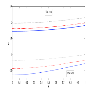
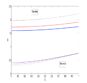
Figure 3: Effects of (a) positively charged dusts $(\delta)$, (b) the external magnetic field $(\omega_{cp})$, and (c) the ratio of negative and positive ion masses $(m)$ on the DIC modes given by Eq. (27) are shown. In each subfigure, the upper (three thick lines) and the lower (three thin lines) curves, respectively, correspond to the fast and slow DIC modes. For the subfigures (a) to (c), different values of the parameters $\delta,~{}\omega_{cp}$, and $m$, as well as the corresponding fixed parameter values are considered as the same as in Figs. 1, 1 1 respectively.

IV Derivation of KdV equation

In the linear analysis, we have neglected some interesting physics contained in the second-order perturbation terms like $n_{j1}v_{j1}$ etc. or some higher-order terms. These are, indeed, important when the wave grows in amplitude. In this section, we are interested to consider the nonlinear propagation (oblique to the magnetic field) of small but finite amplitude electrostatic DIA waves in a magnetized dusty pair-ion plasma. We follow the standard reductive perturbation technique in which the stretched coordinates are defined as misra-samanta-jpp

$$\begin{split}\xi&=\epsilon^{1/2}({\hat{\kappa}}\cdot\mathbf{r}-Mt)\\ &=\epsilon^{1/2}(l_{x}x+l_{y}y+l_{z}z-Mt),\\ &\tau=\epsilon^{3/2}t,\end{split}$$ (30)

where $\epsilon$ is a small scaling parameter $(\lesssim 1)$ measuring the weakness of perturbations and $M$ is the nonlinear wave speed (relative to the rest frame), normalized by $c_{s}$, to be determined later. Also, $\hat{\kappa}$ is the unit vector along the direction of the wave propagation with $l_{x}$, $l_{y}$, $l_{z}$ denoting its direction cosines along $x$, $y$ and $z$ axes respectively. The dynamical variables are expanded as misra-samanta-jpp

$$\begin{split}n_{j}&=1+\epsilon n_{j}^{(1)}+\epsilon^{2}n_{j}^{(2)}+\cdots,\\ v_{jx,y}&=\epsilon^{3/2}v_{jx,y}^{(1)}+\epsilon^{2}v_{jx,y}^{(2)}+\cdots,\\ v_{jz}&=\epsilon v_{jz}^{(1)}+\epsilon^{2}v_{jz}^{(2)}+\cdots,\\ \phi&=\epsilon\phi^{(1)}+\epsilon^{2}\phi^{(2)}+\cdots.\end{split}$$ (31)

Note that in the expansions (31), the first-order perturbations for the transverse velocity components of the ion fluids appear in higher-orders of $\epsilon$ than that for the parallel components. For the nonlinear DIA waves, this anisotropy is introduced due to the fact that the ion gyro-motion (perpendicular to the magnetic field) is treated as a higher-order effect than the motion parallel to the magnetic field mi-bains-pop ; zk-misra-pop .

Next, we substitute the expressions from Eqs. (30) and (31) into Eqs. (5)-(7), and equate different powers of $\epsilon$. Thus, from Eq. (5), equating successively the coefficients of $\epsilon^{3/2}$, $\epsilon^{2}$ and $\epsilon^{5/2}$, we obtain

$$n^{(1)}_{j}=\frac{l_{z}}{M}v^{(1)}_{jz},$$ (32)

$$v^{(1)}_{jx}=-\frac{l_{y}}{l_{x}}v^{(1)}_{jy},$$ (33)

$$-M\frac{\partial n^{(2)}_{j}}{\partial\xi}+\frac{\partial n^{(1)}_{j}}{\partial\tau}+l_{x}\frac{\partial v^{(2)}_{jx}}{\partial\xi}+l_{y}\frac{\partial v^{(2)}_{jy}}{\partial\xi}+l_{z}\frac{\partial v^{(2)}_{jz}}{\partial\xi}$$

$$+l_{z}\frac{\partial\left({n^{(1)}_{j}}{v^{(1)}_{jz}}\right)}{\partial\xi}=0.$$ (34)

From the $x$ and $y$-components of Eq. (6) for positive ions, and equating the coefficients of $\epsilon^{3/2}$ and $\epsilon^{2}$, we successively obtain

$$0=-ml_{x,y}\frac{\partial\phi^{(1)}}{\partial\xi}\pm\omega_{cp}v^{(1)}_{p(y,x)}-\frac{5}{3}ml_{x,y}\frac{\partial n^{(1)}_{p}}{\partial\xi},$$ (35)

$$M\frac{\partial v^{(1)}_{p(x,y)}}{\partial\xi}=\mp\omega_{cp}v^{(2)}_{p(y,x)}.$$ (36)

Next, from the $z$-component of Eq. (6) for positive ions, and equating the coefficients of $\epsilon^{3/2}$ and $\epsilon^{5/2}$, we, respectively, obtain

$$v^{(1)}_{pz}=\frac{ml_{z}}{M}\left(\phi^{(1)}+\frac{5}{3}n^{(1)}_{p}\right),$$ (37)

$$-M\frac{\partial v^{(2)}_{pz}}{\partial\xi}+\frac{\partial v^{(1)}_{pz}}{\partial\tau}+l_{z}v^{(1)}_{pz}\frac{\partial v^{(1)}_{pz}}{\partial\xi}=$$

$$ml_{z}\left[-\frac{\partial\phi^{(2)}}{\partial\xi}+\frac{5}{9}\left(n^{(1)}_{p}\frac{\partial n^{(1)}_{p}}{\partial\xi}-3\frac{\partial n^{(2)}_{p}}{\partial\xi}\right)\right].$$ (38)

Similarly, from the $x$ and $y$-components of Eq. (6) for negative ions, and equating the coefficients of $\epsilon^{3/2}$ and $\epsilon^{2}$, we successively obtain

$$0=l_{x,y}\frac{\partial\phi^{(1)}}{\partial\xi}\mp\omega_{cn}v^{(1)}_{n(y,x)}-\frac{5}{3}Tl_{x,y}\frac{\partial n^{(1)}_{n}}{\partial\xi},$$ (39)

$$M\frac{\partial v^{(1)}_{n(x,y)}}{\partial\xi}=\pm\omega_{cn}v^{(2)}_{n(y,x)}.$$ (40)

Also, from the $z$-component of Eq. (6) for negative ions, and equating the coefficients of $\epsilon^{3/2}$ and $\epsilon^{5/2}$, we obtain

$$v^{(1)}_{nz}=-\frac{l_{z}}{M}\left(\phi^{(1)}-\frac{5}{3}Tn^{(1)}_{n}\right),$$ (41)

$$-M\frac{\partial v^{(2)}_{nz}}{\partial\xi}+\frac{\partial v^{(1)}_{nz}}{\partial\tau}+l_{z}\left(v^{(1)}_{nz}\frac{\partial v^{(1)}_{nz}}{\partial\xi}-\frac{\partial\phi^{(2)}}{\partial\xi}\right)$$

$$=\frac{5}{9}Tl_{z}\left(n^{(1)}_{n}\frac{\partial n^{(1)}_{n}}{\partial\xi}-3\frac{\partial n^{(2)}_{n}}{\partial\xi}\right).$$ (42)

Furthermore, from the Poisson’s equation, i.e., Eq. (7), and equating the coefficients of $\epsilon$ and $\epsilon^{2}$, we successively have

$$n^{(1)}_{n}=\mu n^{(1)}_{p},$$ (43)

$$\frac{\partial^{2}\phi^{(1)}}{\partial\xi^{2}}=n^{(2)}_{n}-\mu n^{(2)}_{p}.$$ (44)

First-order perturbations and nonlinear wave speed

From Eqs. (32), (37) and (41), after eliminating $v^{(1)}_{jz}$ we have

$$n^{(1)}_{j}=\pm l^{2}_{z}\lambda_{j}\phi^{(1)},$$ (45)

where the $\pm$ stand for positive $(j=p)$ and negative ions $(j=n)$. Also, $\lambda_{p}={3m}/\left({3M^{2}-5ml^{2}_{z}}\right)$ and $\lambda_{n}=3/\left({3M^{2}-5Tl^{2}_{z}}\right)$. For typical plasma parameters with $m>1$ and $T<1$, the coefficients $\lambda_{p}$ and $\lambda_{n}$ are both positive for $M^{2}>5ml^{2}_{z}/3$. The latter will be validated from the expression of $M$, to be obtained shortly. This implies that the first-order density perturbations corresponding to the positive and negative ion fluids are of opposite in sign. The same also applies to the perturbations of the velocity components of the ion fluids [See the expressions (47) below]. From Eqs. (35), (39) and (45), after eliminating $n_{j}^{(1)}$, we obtain $(j=p,n)$

$$v^{(1)}_{j(x,y)}=\mp l_{y,x}\frac{M^{2}\lambda_{j}}{\omega_{cj}}\frac{\partial\phi^{(1)}}{\partial\xi},$$ (46)

where the $\mp$ stand for $x$ and $y$-components. Also, from Eqs. (32) and (45), we have

$$v^{(1)}_{jz}=\pm Ml_{z}\lambda_{j}\phi^{(1)}.$$ (47)

We note that Eq. (46) satisfies Eq. (33) as required. Then from Eqs. (43) and (45), we obtain the expression for the wave speed in the moving frame of reference as

$$M=l_{z}\sqrt{\frac{5}{3}m\left(\frac{1+\mu T}{1+\mu m}\right)}.$$ (48)

From the expression of $\lambda_{p}$, it is clear that $M^{2}\neq{5}ml^{2}_{z}/3$, so $T\neq m$, i.e., the temperature ratio and the mass ratio can not assume the same value. This implies that the present nonlinear theory may not be valid for plasmas with equal mass and temperature of different ion fluids (i.e., the case of $M=T=1$). However, one may consider for laboratory and space plasmas (e.g., as in Ref. pair-ion5 ) that $T<1$ and $m>1$ for which $M^{2}>{5}ml^{2}_{z}/3$. The latter is satisfied for $\lambda_{j}>0$ as mentioned before. Note that Eq. (48) represents the phase speed of the obliquely propagating DIA wave in the $\xi-\tau$ frame of reference, which may correspond to the low-frequency long-wavelength slow mode given by Eq. (23). Interestingly, for $l_{z}=1$, i.e., for wave propagation parallel to the magnetic field, Eq. (48) becomes exactly the same as Eq. (26). We also find that the value of $M$ can be either $>1$ or $<1$ depending on the plasma parameters we consider. For example, for laboratory plasmas as in Table 1, i.e., for $m=3.74$, $T=0.125$, $\mu=0.65$, we can obtain $M=0.7$ or $M=1.12$ when $l_{z}=0.5$ or $l_{z}=0.8$. On the other hand, for space plasma environments as in Table 2, i.e., for $m=10.7$, $T=1$, $\mu=0.5$, we have $M=0.41$ and $1.03$ for $l_{z}=0.2$ and $0.5$ respectively. It is seen that increasing (decreasing) the values of the parameters leads to an increase (decrease) in the value of $M$.

Second-order perturbations

From Eqs. (36) and (40) using Eq. (46) we obtain

$$v^{(2)}_{j(x,y)}=\pm l_{x,y}\frac{M^{3}\lambda_{j}}{\omega^{2}_{cj}}\frac{\partial^{2}\phi^{(1)}}{\partial\xi^{2}},$$ (49)

where the $\pm$ stand for positive $(j=p)$ and negative ions $(j=n)$. Next, from Eq. (34) we eliminate $v_{j}^{(2)}$ using Eq. (49), and use Eq. (32) to substitute the expressions for $n_{j}^{(1)}$ in terms of $\phi_{j}^{(1)}$ in the resulting equation. Thus, we obtain for positive and negative ions as

$$\frac{\partial n^{(2)}_{j}}{\partial\xi}\mp\lambda_{j}l^{2}_{z}\frac{\partial\phi^{(2)}}{\partial\xi}=\pm\lambda_{j}^{2}\frac{Mm_{j}}{m_{n}}\left[M^{2}\frac{\left(1-l^{2}_{z}\right)}{\omega^{2}_{cj}}\frac{\partial^{3}\phi^{(1)}}{\partial\xi^{3}}\right.$$

$$\left.+2l_{z}^{2}\frac{\partial\phi^{(1)}}{\partial\tau}\pm\lambda_{j}Ml^{4}_{z}\left(27-\frac{5m_{n}T_{j}l^{2}_{z}}{m_{j}T_{p}M^{2}}\right)\phi^{(1)}\frac{\partial\phi^{(1)}}{\partial\xi}\right],$$ (50)

where the upper (lower) sign stands for $j=p~{}(j=n)$.

KdV equation

Substituting the expressions for $\partial n_{j}^{(2)}/\partial\xi$, $j=p,n$, to be obtained from Eq. (50) into Eq. (44), and noting that coefficient of $\phi^{(2)}$ vanishes by Eq. (48), we obtain the following KdV equation

$$\frac{\partial\Phi}{\partial\tau}+A\Phi\frac{\partial\Phi}{\partial\xi}+B\frac{\partial^{3}\Phi}{\partial\xi^{3}}=0,$$ (51)

where $\Phi\equiv\phi^{(1)}\lesssim 1$, such that $\epsilon\phi^{(1)}<1$. The coefficients of nonlinearity and dispersion are, respectively, given by

$$A =\frac{1}{2\sqrt{1}5}\frac{l_{z}}{(m-T)}\sqrt{\frac{m}{(1+\mu m)(1+\mu T)}}$$

$$\times\left[\left(1+\mu^{2}T\right)\left(1+\mu m\right)-9\left(1+\mu^{2}m\right)\left(1+\mu T\right)\right],$$

$$B =\frac{5\sqrt{5}}{6\sqrt{3}}l_{z}\sqrt{m}\frac{(1+\mu T)^{3/2}}{(1+\mu m)^{5/2}}$$ (53)

$$\times\left[\frac{\mu(m-T)^{2}}{(1+\mu T)^{2}}+\frac{(1-l^{2}_{z})(1+m^{3}\mu)}{\omega_{cp}\omega_{cn}}\right].$$

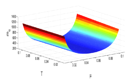
Figure 4: Typical variations of the critical mass $m_{c}$ are shown with respect to the density and the temperatures ratios $\mu$ and $T$.

Inspecting on the expressions for $A$ and $B$ we find that $B$ is always positive. However, $A\gtreqqless 0$ according to when $m\gtreqqless m_{c}$, where $m_{c}$ is a critical value of $m$ given by

$$m_{c}=\frac{8+\mu T(9-\mu)}{\mu\left[1-\mu(9+8\mu T)\right]}.$$ (54)

In order that $m_{c}>0$, we must have $T<T_{c}\equiv(1-9\mu)/8\mu^{2}<1$ and $\mu<1/9$. For typical plasma parameters (See Tables 1 and 2) with $m>1$ and $T<T_{c},\mu<1/9$, the values of $m_{c}$ become much larger than unity (e.g., for $\mu=T=0.1$, we have $m_{c}=879.2$), and so the dispersion coefficient $A$ is always negative for $m\ll m_{c}$. Thus, typical laboratory and space plasmas as in Tables 1 and 2 with a pair of ions may support only rarefactive DIA solitons. On the other hand, for $m\sim m_{c}$ the KdV equation (51) fails to describe the evolution of DIA waves. In this case, one has go for higher-order corrections to derive a modified KdV equation which may admit a compressive DIA soliton solution in plasmas with $m\gg 1$, i.e., with much heavier negative ions than positive ones rosenberg2009 . Typical variations of $m_{c}$ with respect to $\mu$ and $T$ are shown in Fig. 4. It is clear that for a fixed $\mu$ as $T$ increases, the value of $m_{c}$ increases. However, for a fixed $T$, $m_{c}$ decreases (increases) in the subinterval $0.01\lesssim\mu\lesssim 0.07$ $(0.07<\mu\lesssim 0.11)$. Furthermore, the case of $m\gg m_{c}$ for which $A>0$ may not be relevant for the present study. We also note that this critical value of $m$ may not appear in a magnetized pair-ion plasma without stationary charged dusts, because in this case, the term in the square brackets in the expression of $A$ becomes $-8(1+m)(1+T)$, i.e., negative. Thus, in magnetized pure pair-ion plasmas, there may exist DIA solitary waves with only the negative potential.

A stationary solitary solution of Eq. (51) can be obtained by applying a transformation $\eta=\xi-U_{0}\tau$ to Eq. (51), where $U_{0}$ is the constant phase speed normalized by $c_{s}$, and imposing the boundary conditions for localized perturbations, namely, $\phi$, $d\phi/d\xi$, $d^{2}\phi/d\xi^{2}\rightarrow 0$ as $\xi\rightarrow\pm\infty$, as

$$\Phi=\Phi_{m}\text{sech}^{2}(\eta/w),$$ (55)

where $\Phi_{m}=3U_{0}/A$ is the finite amplitude and $w=\sqrt{4B/U_{0}}$ is the finite width of the soliton with $B>0$.

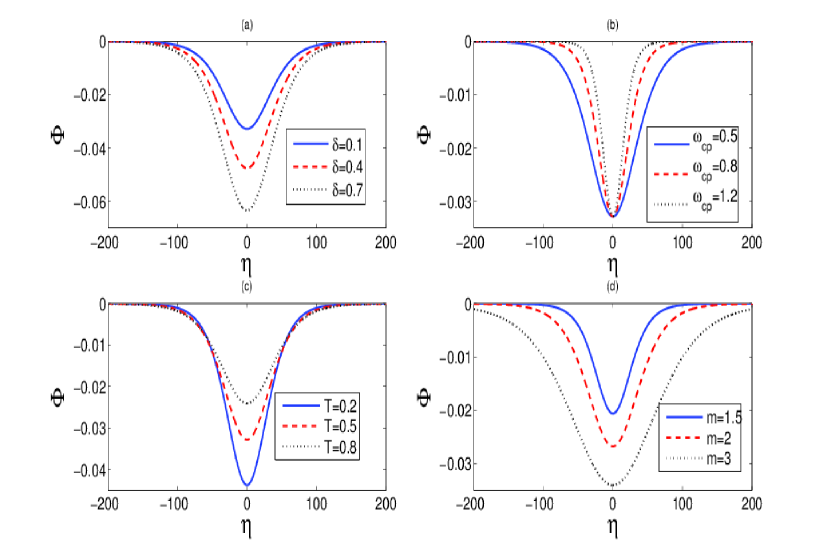
Figure 5: Stationary soliton solution [Eq. (55)] of the KdV equation (51) at $\tau=0$, and with $U_{0}=0.2$ is plotted against $\eta$. Subplots (a) to (d), respectively, show the effects of (a) positively charged dusts $(\delta)$, (b) the external magnetic field $(\omega_{cp})$, (c) the negative to positive ion temperature ratio $(T)$, and (d) the ratio of negative and positive ion masses $(m)$. The corresponding fixed parameter values are as in subfigures. 1, 1, 1 and 1 respectively.

Relying on the coefficients $A$ and $B$ of the KdV equation (51), we study the properties of the rarefactive solitons (55) (See Fig. 5) for different values of the parameters as in Fig. 1. It is found that, for fixed values of the mass ratio $m=2$, the temperature ratio $T=0.5$, and the magnetic field given by $\omega_{cp}=0.5$, as the charged dust concentration increases, both the amplitude and width of the soliton increases. Figure 5(b) shows that the magnetic field has influence only on the width of the soliton, since the effect of $B_{0}$ is only entered into the dispersion coefficient $B$. A stronger magnetic field reduces the width, while the amplitude remains constant. The influences of the temperature ratio $(T)$ on the amplitude and width of the soliton are shown in Fig. 5(c). It is found that the amplitude decreases significantly, while the width increases as the value of $T$ increases. A significant decrease in the amplitude as well as a significant increase in the width of the solitons are found with increasing values of the mass ratio $m$ [Fig. 5(d)]. Furthermore, since both the nonlinear and dispersion coefficients $A$ and $B$ are proportional to the obliqueness parameter $l_{z}$, its effect is to decrease (increase) the amplitude (width) of the DIA soliton.

V Derivation of mKdV equation

In the previous section we noticed that when $m=m_{c}$, the nonlinear coefficient of the KdV equation (51) vanishes, i.e., $A=0$. In this situation, Eq. (51) fails to describe the evolution of small-amplitude DIA waves. Thus, for values of $m\sim m_{c}$, we derive a modified KdV equation using the same reductive perturbation technique as in the previous section. We also take the same stretched coordinates for space and time. However, the dependent variables are expanded in a different manner as

$$\begin{split}n_{j}&=1+\epsilon^{1/2}n_{j}^{(1)}+\epsilon n_{j}^{(2)}+\epsilon^{3/2}n_{j}^{(3)}+\cdots,\\ v_{jx,y}&=\epsilon v_{jx,y}^{(1)}+\epsilon^{3/2}v_{jx,y}^{(2)}+\epsilon^{2}v_{jx,y}^{(3)}+\cdots,\\ v_{jz}&=\epsilon^{1/2}v_{jz}^{(1)}+\epsilon v_{jz}^{(2)}+\epsilon^{3/2}v_{jz}^{(3)}+\cdots,\\ \phi&=\epsilon^{1/2}\phi^{(1)}+\epsilon\phi^{(2)}+\epsilon^{3/2}\phi^{(3)}+\cdots.\end{split}$$ (56)

We substitute the expansions (56) and the stretched coordinates (30) into Eqs. (5)-(7), and equate different powers of $\epsilon$ successively. In the lowest orders of $\epsilon$, i.e., $\epsilon$ and $\epsilon^{1/2}$ we obtain the same expressions for the first-order perturbations and the nonlinear wave speed $M$ as Eqs. (45)-(48). However, from Eq. (5) equating the coefficients of $\epsilon^{3/2}$ and $\epsilon^{2}$, we successively obtain

$$Mn^{(2)}_{j}-l_{z}v^{(2)}_{jz}=l_{x}v^{(1)}_{jx}+l_{y}v^{(1)}_{jy}+l_{z}n^{(1)}_{j}v^{(1)}_{jz},$$ (57)

$$-M\frac{\partial n^{(3)}_{j}}{\partial\xi}+\frac{\partial n^{(1)}_{j}}{\partial\tau}+l_{x}\frac{\partial}{\partial\xi}\left(n^{(1)}_{j}v^{(1)}_{jx}+v^{(2)}_{jx}\right)$$

$$+l_{y}\frac{\partial}{\partial\xi}\left(n^{(1)}_{j}v^{(1)}_{jy}+v^{(2)}_{jy}\right)$$

$$+l_{z}\frac{\partial}{\partial\xi}\left(n^{(1)}_{j}v^{(2)}_{jz}+n^{(2)}_{j}v^{(1)}_{jz}+v^{(3)}_{jz}\right)=0.$$ (58)

Next, from the $x$ and $y$-components of Eq. (6) for positive ions, and equating the coefficients of $\epsilon^{3/2}$, we have

$$M\frac{\partial v^{(1)}_{p(x,y)}}{\partial\xi} =ml_{x,y}\frac{\partial\phi^{(2)}}{\partial\xi}\mp\omega_{cp}v^{(2)}_{p(y,x)}+\frac{5}{3}ml_{x,y}\frac{\partial n^{(2)}_{p}}{\partial\xi}$$ (59)

$$-\frac{5}{18}ml_{x,y}\frac{\partial(n^{(1)}_{p})^{2}}{\partial\xi},$$

where the $\mp$ stand for the $x$ and $y$-components respectively. Furthermore, from the $z$-component of Eq. (6) for positive ions, equating the coefficients of $\epsilon^{3/2}$ and $\epsilon^{2}$ we have

$$-Mv^{(2)}_{pz}+\frac{l_{z}}{2}(v^{(1)}_{pz})^{2}=-ml_{z}\phi^{(2)}$$

$$+\frac{5}{3}ml_{z}\left[\frac{1}{6}\left(n^{(1)}_{p}\right)^{2}-n^{(2)}_{p}\right],$$ (60)

$$-M\frac{\partial v^{(3)}_{pz}}{\partial\xi}+\frac{\partial v^{(1)}_{pz}}{\partial\tau}+\left(l_{x}v^{(1)}_{px}+l_{y}v^{(1)}_{py}\right)\frac{\partial v^{(1)}_{pz}}{\partial\xi}$$

$$+l_{x}\frac{\partial(v^{(1)}_{pz}v^{(2)}_{pz})}{\partial\xi}=-ml_{z}\frac{\partial\phi^{(3)}}{\partial\xi}$$

$$+\frac{5}{9}ml_{z}\left[\frac{\partial(n^{(1)}_{p}n^{(2)}_{p})}{\partial\xi}-3\frac{\partial n^{(3)}_{p}}{\partial\xi}-\frac{2}{9}\frac{\partial(n^{(1)}_{p})^{3}}{\partial\xi}\right].$$ (61)

Similar expressions for the negative ions can also be obtained. Thus, from the $x$ and $y$-components of Eq. (6), equating the coefficients of $\epsilon^{3/2}$, we successively obtain

$$-M\frac{\partial v^{(1)}_{n(x,y)}}{\partial\xi}=l_{x,y}\frac{\partial\phi^{(2)}}{\partial\xi}\mp\omega_{cn}v^{(2)}_{n(y,x)}-\frac{5}{3}Tl_{x,y}\frac{\partial n^{(2)}_{n}}{\partial\xi}$$

$$+\frac{5}{18}Tl_{x,y}\frac{\partial(n^{(1)}_{p})^{2}}{\partial\xi},$$ (62)

where the $\mp$ stand for the $x$ and $y$-components respectively. From the $z$-component of Eq. (6) equating the coefficients of $\epsilon^{3/2}$ and $\epsilon^{2}$ we have

$$-\frac{M}{l_{z}}v^{(2)}_{nz}+\frac{1}{2}\left(v^{(1)}_{nz}\right)^{2}=\phi^{(2)}+\frac{5}{3}T\left[\frac{1}{6}\left(n^{(1)}_{n}\right)^{2}-n^{(2)}_{n}\right],$$ (63)

$$-M\frac{\partial v^{(3)}_{nz}}{\partial\xi}+\frac{\partial v^{(1)}_{nz}}{\partial\tau}+\left(l_{x}v^{(1)}_{nx}+l_{y}v^{(1)}_{ny}\right)\frac{\partial v^{(1)}_{nz}}{\partial\xi}$$

$$+l_{x}\frac{\partial(v^{(1)}_{nz}v^{(2)}_{nz})}{\partial\xi}=ml_{z}\frac{\partial\phi^{(3)}}{\partial\xi}$$

$$+\frac{5}{9}Tl_{z}\left[\frac{\partial(n^{(1)}_{n}n^{(2)}_{n})}{\partial\xi}-3\frac{\partial n^{(3)}_{n}}{\partial\xi}-\frac{2}{9}\frac{\partial(n^{(1)}_{n})^{3}}{\partial\xi}\right].$$ (64)

Furthermore, from Eq. (7) equating the coefficients of $\epsilon$ and $\epsilon^{3/2}$ we obtain

$$n^{(2)}_{n}=\mu n^{(2)}_{p},$$ (65)

$$\frac{\partial^{2}\phi^{(1)}}{\partial\xi^{2}}=n^{(3)}_{n}-\mu n^{(3)}_{p}.$$ (66)

Second-order perturbations

From Eqs. (57), (60) and (63) solving for $n^{(2)}_{j}$ and $v^{(2)}_{jz}$ $(j=p,n)$, and substituting the corresponding first-order quantities from Eqs. (45) and (46) wherever necessary, we obtain

$$n^{(2)}_{j}=\zeta_{j}\lambda_{j}l_{z}^{2}\phi^{(2)}+\frac{m_{j}}{2m_{n}}\lambda^{3}_{j}l_{z}^{4}\left(3M^{2}-\frac{5}{9}\frac{m_{n}T_{j}}{m_{j}T_{p}}l^{2}_{z}\right)(\phi^{(1)})^{2},$$ (67)

$$v^{(2)}_{jz} =3\zeta_{j}M\lambda_{j}l_{z}\phi^{(2)}$$ (68)

$$+\frac{M}{18}\frac{m_{j}}{m_{n}}\lambda^{3}_{j}l_{z}^{3}\left(9M^{2}+25\frac{m_{n}T_{j}}{m_{j}T_{p}}l^{2}_{z}\right)(\phi^{(1)})^{2},$$

where $\zeta_{p}=1$ and $\zeta_{n}=-1$. Similarly, we solve for $v^{(2)}_{jx}$ and $v^{(2)}_{jy}$, $j=p,n$, from Eqs. (59) and (62) to obtain

$$v^{(2)}_{jx}= -\frac{m_{n}l_{y}}{m_{j}\omega_{cj}}\left(1+\frac{5T_{j}}{3T_{p}}l_{z}^{2}\lambda_{j}\right)\frac{\partial\phi^{(2)}}{\partial\xi}+\zeta_{j}M^{3}l_{x}\frac{\lambda_{j}}{\omega^{2}_{cj}}\frac{\partial^{2}\phi^{(1)}}{\partial\xi^{2}}$$ (69)

$$-\zeta_{j}\frac{5l_{y}}{54}\frac{T_{j}}{T_{p}}\frac{l_{z}^{4}\lambda^{2}_{j}}{\omega_{cj}}\left[\lambda_{j}\left(27M^{2}-5\frac{m_{n}T_{j}}{m_{j}T_{p}}l_{z}^{2}\right)-3\frac{m_{n}}{m_{j}}\right]$$

$$\times\frac{\partial(\phi^{(1)})^{2}}{\partial\xi},$$

$$v^{(2)}_{jy}= \frac{m_{n}l_{x}}{m_{j}\omega_{cj}}\left(1+\frac{5T_{j}}{3T_{p}}l_{z}^{2}\lambda_{j}\right)\frac{\partial\phi^{(2)}}{\partial\xi}+\zeta_{j}M^{3}l_{y}\frac{\lambda_{j}}{\omega^{2}_{cj}}\frac{\partial^{2}\phi^{(1)}}{\partial\xi^{2}}$$ (70)

$$+\zeta_{j}\frac{5l_{x}}{54}\frac{T_{j}}{T_{p}}\frac{l_{z}^{4}\lambda^{2}_{j}}{\omega_{cj}}\left[\lambda_{j}\left(27M^{2}-5\frac{m_{n}T_{j}}{m_{j}T_{p}}l_{z}^{2}\right)-3\frac{m_{n}}{m_{j}}\right]$$

$$\times\frac{\partial(\phi^{(1)})^{2}}{\partial\xi}.$$

mKdv equation

We eliminate $v^{(3)}_{jz}$ and $n^{(3)}_{j}$ from Eqs. (58), (61), (64) and (66) and note that the coefficients of $\phi^{(3)}$ and $\partial\left(\phi^{(1)}\phi^{(2)}\right)/\partial\xi$ vanish, respectively, by means of Eq.(48) and the critical condition $A=0$. Thus, one obtains the following mKdV equation

$$\frac{\partial\Phi}{\partial\tau}+A^{\prime}\Phi^{2}\frac{\partial\Phi}{\partial\xi}+B\frac{\partial^{3}\Phi}{\partial\xi^{3}}=0,$$ (71)

where $\Phi\equiv\phi^{(1)}$. The dispersion coefficient is the same as in Eq. (51), however, the coefficient of nonlinearity which appears as a higher-order effect, is given by

$$A^{\prime}= \frac{1}{10}\frac{l_{z}}{\mu^{3}}\left[\frac{3}{5}m(1+\mu T)\right]^{1/2}\frac{(1+\mu m)^{3/2}}{(m-T)^{3}}$$ (72)

$$\times\left[\frac{45}{2}\left(\frac{1+\mu T}{1+\mu m}\right)\left(\mu^{4}m^{2}-1\right)+3\left(\mu^{4}mT-1\right)\right.$$

$$\left.+\frac{1}{2}\frac{\left(\mu^{4}T^{2}-1\right)(1+\mu m)}{1+\mu T}\right.$$

$$\left.+\frac{2}{3}\frac{\mu(1+\mu^{3}T)(m-T)}{1+\mu T}\right].$$

Equation (71) describes the evolution of DIA waves in pair-ion plasmas in the critical condition $m\sim m_{c}\gg 1$, i.e., in plasmas containing much heavier negative ions than the positive ions. A stationary soliton solution of Eq. (71) is obtained by applying a transformation $\eta=\xi-U_{0}\tau$ as

$$\Phi=\Psi~{}\text{sech}\left(\eta/W\right),$$ (73)

where $\Psi=6U_{0}/A^{\prime}$ is the amplitude and $W=\sqrt{B/U_{0}}$ is the width of the mKdV soliton with $B>0$. Inspecting on the coefficients $A^{\prime}$ and $B$ we find that for typical values of the parameters with $m\sim m_{c}\gg 1$, $\omega_{cp}\sim 1$, $T<T_{c}<1$ and $\mu<1/9$, we have $A<1$ and $B\gg 1$. Since soliton formation is due to a nice balance between the nonlinear and the dispersion coefficients, one should not expect $B\gg A$. Thus, in order to have appreciable values of $A$ and $B$, we consider $\omega_{cp}\gg 1$. Figure 6 shows the characteristic features of the mKdV soliton with the variations of (a) $\delta$, (b) $\omega_{cp}$ and (c) $T$. We find that as $\delta$ increases, the amplitude of the soliton increases, while the width decreases for $\delta\lesssim 0.91$. As in the case of KdV solitons, the effect of the external magnetic field, characterized by $\omega_{cp}$, is to decrease the soliton width only, since $A$ is independent of $\omega_{cp}$. We also find that as the temperature ratio $T$ increases, the width increases, while the amplitude of the soliton decreases. Similar to the KdV solitons, the effects of $l_{z}$ is to decrease (increase) the amplitude (width) of the mKdV DIA solitons.

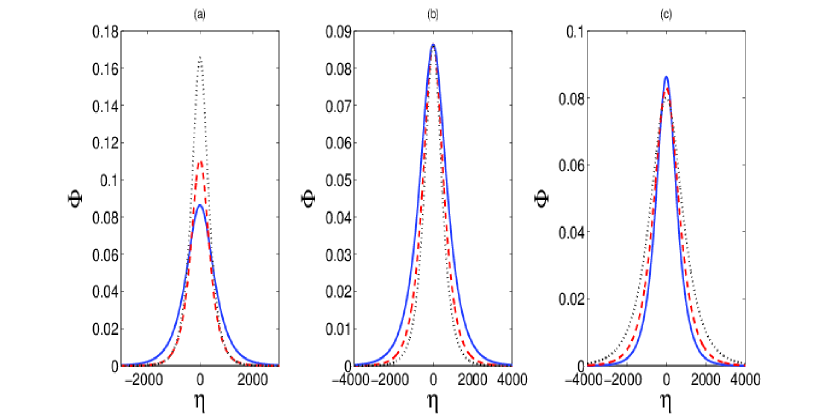
Figure 6: Stationary soliton solution [Eq. (73)] of the mKdV equation (71) at $\tau=0$, and with $U_{0}=0.001$ is shown with the variations of (a) $\delta$: $\delta=0.9$ (solid line), $0.91$ (dashed line) and $0.92$ (dotted line); the other parameter values are $T=0.1$, $l_{z}=0.8$, $\omega_{cp}=200$ and $m=m_{c}-10$ (b) $\omega_{cp}$: $\omega_{cp}=150$ (solid line), $200$ (dashed line) and $250$ (dotted line); the other parameter values are $\delta=0.9$, $T=0.1$, $l_{z}=0.8$ and $m=m_{c}-10$ (c) $T$: $T=0.1$ (solid line), $0.3$ (dashed line) and $0.5$ (dotted line); the other parameter values are $\delta=0.9$, $l_{z}=0.8$, $\omega_{cp}=200$ and $m=m_{c}-10$.

VI Discussion and conclusion

We have investigated the characteristics of small-amplitude electrostatic perturbations propagating obliquely to the external magnetic field in an electron-free dusty pair-ion plasma.

Table 1: Laboratory plasma parameters

$m_{p}$	$39m_{\text{proton}}=6.5\times 10^{-23}$ g
$m_{n}$	$146m_{\text{proton}}=2.4\times 10^{-22}$ g
$T_{p}$	$0.2~{}$ev$=2321~{}$K
$T_{n}$	$0.025~{}$ev$=290.12~{}$K
$n_{n0}$	$2\times 10^{9}$ cm-3
$n_{p0}$	$1.3\times 10^{9}$ cm-3
$n_{d0}$	$2\times 10^{6}$ cm-3
$\phi_{s}$	$0.1$ v$=3.3\times 10^{-4}$ statv
$R$	$5.04~{}\mu$m$=5.04\times 10^{-4}~{}$cm
$z_{d}$	$\sim R\phi_{s}/e\sim 350$
$B_{0}$	$0.3~{}$T$=3000~{}$G

Table 2: Space plasma parameters

$m_{p}$	$28m_{\text{proton}}=4.7\times 10^{-23}$ g
$m_{n}$	$300m_{\text{proton}}=5.02\times 10^{-22}$ g
$T_{p}$	$200~{}$K
$T_{n}$	$200~{}$K
$n_{n0}$	$2\times 10^{6}$ cm-3
$n_{p0}$	$10^{6}$ cm-3
$z_{d}n_{d0}$	$10^{6}$ cm-3
$\phi_{s}$	$0.7$ v$=2.3\times 10^{-3}$ statv
$R$	$0.6~{}$nm$=6\times 10^{-8}~{}$cm
$B_{0}$	$0.5~{}$G

In the linear regime (i.e., the very small-amplitude limit), we have Fourier analyzed the basic (linear) equations, and found that low-frequency (in comparison with the ion-cyclotron frequency) long-wavelength oblique slow and fast modes can propagate as dust ion-acoustic (DIA) and dust ion-cyclotron (DIC)-like waves. The properties of these waves are studied with the effects of (i) obliqueness of propagation angle with the magnetic field $(\theta)$, (ii) charged dust impurity in the plasma $(\delta)$, (iii) the static magnetic field $(\omega_{cp})$, (iv) the adiabatic ion temperature ratio $(T)$, and (v) the ion mass ratio $(m)$ (See Fig. 1). We show that the frequency gap between the two fast and slow modes decrease as $k\rightarrow 0$ by the effects of $\delta$ and $T$. The frequencies of these modes are significantly altered under the influence of the external magnetic field and different masses of ions $(m\neq 1)$. Furthermore, a simultaneous increase in the frequencies of both the modes is observed for higher values of the temperature ratio $T$, and the magnetic field characterized by $\omega_{cp}$. Also, for a wave number higher than its critical value, an opposite trend of change in the frequencies of the modes is seen to occur by the effects of $\delta$ and the mass ratio $m$ $(>1)$. A similar analysis has also been carried out for the characteristics of DIA and DIC modes [Figs. 2 and 3, which, in particular, appear for wave propagation parallel and perpendicular to the magnetic field.

In the nonlinear theory, special emphasis is given to study the oblique propagation of electrostatic solitary waves. The transverse velocity perturbations of the ion fluids are assumed to be of higher-order effects than that for the parallel components. Such anisotropy is introduced because, the ion gyro-motion is treated as a higher-order effect than the motion along the magnetic field. Thus, we are interested to consider the nonlinear propagation of DIA solitary waves (instead of DIC waves). A standard reductive perturbation technique is used to derive a KdV equation which describes the evolution of electrostatic DIA perturbations. We have shown that the phase speed of the nonlinear wave in the moving frame of reference corresponds to that of the obliquely propagating low-frequency linear DIA mode. Furthermore, it is found that the dispersion coefficient $B$ of the KdV equation is always positive, while the nonlinear coefficient $A$ can be negative or positive depending on whether the mass ratio $m$ is below or above its critical value $m_{c}$. The latter typically depends on the temperature ratio $T$ and the density ratio $\mu$. It is found that for appreciable values of $m_{c}~{}(>0)$, the conditions $T<T_{c}\equiv(1-9\mu)/8\mu^{2}<1$ and $\mu<1/9$ must be satisfied, and thus, one finds $m_{c}\gg 1$. The latter corresponds to plasmas with much heavier negative ions than the positive ones $(m\gg 1)$. However, for typical laboratory and space plasma parameters as in Tables 1 and 2, $m\ll m_{c}$ and so the KdV equation admits only raraefactive DIA solitons. The formation of compressive solitary waves may be possible for $m\gg m_{c}$, however, those plasma regimes may not be relevant in laboratory and space environments. On the other hand, for values of $m$ close to $m_{c}$, i.e., $m\sim m_{c}\gg 1$, the KdV equation fails to describe the evolution of DIA solitons. In this case, we have derived a modified KdV equation which is shown to admit only compressive DIA solitons in pair-ion plasmas with much heavier negative ions than the positive ones. It is to be noted that the critical mass $m_{c}$ for which the nonlinear coefficient $A$ changes its sign may not appear in a magnetized pair-ion plasma without any charged dust impurity. In this case solitary waves may exist with only the negative potential. Thus, charged dust grains in the background plasma play important roles for the existence of compressive or rarefactive solitons.

Table 3: Frequency estimates for laboratory plasmas

Wave	$k\lambda_{D}/\lambda$ (cm)	$\omega_{\text{fast}}/2\pi$ (kHz)	$\omega_{\text{slow}}/2\pi$ (kHz)
	$0.01/4.7$	$48.5$	$10.5$
Oblique	$0.2/0.23$	$366$	$28.6$
	$0.7/0.07$	$125.7$	$28.6$
	$0.01/4.7$	$1.4\times 10^{3}$	$9.4$
DIA	$0.2/0.23$	$1.5\times 10^{3}$	$187.2$
	$0.7/0.07$	$1.8\times 10^{3}$	$551.8$
	$0.01/4.7$	$1.4\times 10^{3}$	$68.5$
DIC	$0.2/0.23$	$1.5\times 10^{3}$	$124.8$
	$0.7/0.07$	$1.6\times 10^{3}$	$363.2$

Table 4: Frequency estimates for space plasmas

Wave	$k\lambda_{D}/\lambda$ (cm)	$\omega_{\text{fast}}/2\pi$ (kHz)	$\omega_{\text{slow}}/2\pi$ (kHz)
	$0.01/4.7$	$31.2$	$0.16$
Oblique	$0.2/0.23$	$626.1$	$0.16$
	$0.7/0.07$	$2.2\times 10^{3}$	$0.16$
	$0.01/4.7$	$1.9\times 10^{3}$	$15.6$
DIA	$0.2/0.23$	$2\times 10^{3}$	$273$
	$0.7/0.07$	$2.7\times 10^{3}$	$826.7$
	$0.01/4.7$	$1.9\times 10^{3}$	$7.8$
DIC	$0.2/0.23$	$1.95\times 10^{3}$	$158.3$
	$0.7/0.07$	$2.2\times 10^{3}$	$522.5$

We, however, mention that the present nonlinear theory of DIA waves is not valid for $T=m$, i.e, when the ratios assume equal values (in particular, for pair-ion plasmas with equal mass and temperature, i.e., $m=T=1$). The stationary soliton solutions of the KdV and mKdV equations are obtained, and their properties are analyzed numerically. It is found that the influence of the external magnetic field is to make the soliton narrower in reducing its width without any change in the amplitude. Similar to the effects of charged dusts, the ion-temperature ratio has also the effect to decrease the soliton amplitude along with a slight increase in its width. The effect of the mass ratio on the soliton profile is almost similar to that of $T$, however, a significant change in the width is seen to occur.

Our theoretical results may be used for experimental verification. For example, we may consider a laboratory plasma pair-ion-charging-experiment ; pair-ion-instability [See Table 1] in which the light positive ions are singly ionized potassium $K^{+}$ and the heavy negative ions are $SF_{6}^{-}$. Thus, the negative to positive ion mass ratio is $m\approx 146/39\approx 3.74$, the negative to positive ion temperature ratio is $T\approx 1/8=0.125$, the negative ion number density is $n_{n0}\sim 2\times 10^{9}$ cm^-3, so that $\mu<1$. Also, according to Kim and Merlino pair-ion-charging-experiment , when $n_{p0}\sim 500n_{e0}$, where $n_{e0}$ is the electron number density, dusts can be positively charged to a surface potential $\phi_{s}\sim 0.1$ V. For a grain of radius $R=5~{}\mu$m, the charge state $z_{d}\sim R\phi_{s}/e\sim 350$. Thus, if $n_{n0}\sim 10^{3}n_{e0}$ and $n_{p0}\sim 650n_{e0}$, so that $\mu=0.7$, then the charge neutrality condition $n_{p0}+z_{d}n_{d0}=n_{n0}$ requires $n_{d0}\sim 2\times 10^{6}$ cm^-3. Suppose that the plasma is immersed in a magnetic field of strength $B_{0}\sim 0.3~{}$T, then for $T_{p}=0.2~{}$ev and $T_{n}=T_{p}/8$, we have, $T=0.12$, $v_{tp}/c_{s}=1.9$, $v_{tn}/c_{s}=0.35$, $\omega_{cp}/\omega_{pn}=0.15$, $\omega_{cn}/\omega_{pn}=0.04$, $\lambda_{D}=0.0074~{}$cm, $\omega_{pn}=4.9\times 10^{6}~{}$s^-1, $c_{s}=3.6\times 10^{5}~{}$cm$/$s. Thus, one can estimate frequencies of different kind of wave modes at different wavelengths $(\lambda=2\pi/k)$ as in Table 3. Alternatively, one can also have similar estimates from the graphical representations of the wave modes as in Figs. 1 to 3. Furthermore, considering the plasma parameters as in Table 1, one can also calculate the nonlinear wave speed given by Eq. (48), the nonlinear and dispersion coefficients $A$ and $B$, as well as the amplitudes and width of the solitons.

On the other hand, Rapp et al. in-situ-Rapp suggested that the presence of sufficiently heavy and numerous negative ions (i.e., $m_{n}>300$ amu and $n_{n0}\gtrsim 50n_{e0}$) can explain their observations of positively charged dusts in the Earth’s mesosphere between 80 and 90 km. Thus, for space plasma environments [See Table 2], e.g., a dusty region at an altitude of about 95 km, we can have $T_{p}\sim T_{n}\sim 200$ K, $m_{n}/m_{p}=300/28\approx 10.7$, $n_{n0}\sim 2\times 10^{6}$ cm^-3, $n_{p0}\sim 10^{6}$ cm^-3, $z_{d}n_{d0}\sim 10^{6}$ cm^-3. Thus, for a magnetic field strength $B_{0}\sim 0.5$ G, we calculate $T=1$, $v_{tp}/c_{s}=3.3$, $v_{tn}/c_{s}=1$, $\omega_{cp}/\omega_{pn}=0.002$, $\omega_{cn}/\omega_{pn}=1.5\times 10^{-4}$, $\lambda_{D}=0.07~{}$cm, $\omega_{pn}=1.1\times 10^{5}~{}$s^-1, $c_{s}=7.4\times 10^{3}~{}$cm$/$s. The frequency estimations of different modes at different wavelength are shown in Table 4. As above we can also estimate the nonlinear wave speed and the soliton characteristics for space plasma parameters as in Table 4.

To conclude, we have studied the effects of immobile positively charged dusts, the obliqueness of propagation, the external magnetic field, the pressure gradient forces and different masses of ions, and their significance for the excitation of oblique DIA and DIC-like waves as well as the nonlinear evolution of KdV and mKdV DIA solitons in magnetized dusty pair-ion plasmas including the case with much heavier negative ions. The theoretical results may be useful for the observation of different kind of wave modes including DIA and DIC waves together with their coupling as well as the nonlinear evolution of DIA solitary waves and solitons in laboratory and space plasmas, e.g., in the Earth’s mesosphere, a magnetized dusty negative-ion plasma region at an altitude of about $95$ km in-situ-Rapp . The results may also be applied to other plasma environments comprising magnetized multi-ions with positively charged dusts, and the parameters satisfy $m\gg 1$ and $T,~{}\mu<1$.

It is to be noted that the inclusion of the effects of ion-dust collisions, ion-drag forces due to positive and negative ions on the charged dusts, as well as the ion-kinematic viscosities in the present model could be another problem of interest, but beyond the scope of the present investigation. Furthermore, the electrostatic disturbances in magnetized pair-ion plasmas with the dynamics and charging of massive dusts could be an another interesting piece of work. However, the processes of charging of dust particles, especially in space plasmas, e.g., in mesospheric nanoparticles are much more complicated that hitherto assumed in-situ-Rapp . Thus, more in situ, laboratory, and theoretical investigations are needed to study the size distribution and charging properties of mesospheric nanoparticles, and their significance for the propagation of DIA waves and other nonlinear phenomena.

References

- (1) E. Yabe and K. Takahashi, Appl. Phys. Lett. 65, 694 (1994).
- (2) W. Oohara, D. Date, and R. Hatakeyama, Phys. Rev. Lett. 95, 175003 (2005).
- (3) H. Saleem, Phys. Plasmas 14, 014505 (2007).
- (4) A. P. Misra, N. C. Adhikary, and P. K. Shukla, Phys. Rev. E 86, 056406 (2012).
- (5) H. U. Rehman, Chin. Phys. Lett. 29, 65201 (2012).
- (6) S. Ghosh, N. Chakrabarti, M. Khan, and M. R. Gupta, PRAMANA-J. Phys. 80, 283 (2013).
- (7) S. Mahmood, H. U. Rehman, and H. Saleem, Phys. Scr. 80, 035502 (2009).
- (8) A. P. Misra and N. C. Adhikary, Phys. Plasmas 20, 102309 (2013).
- (9) N. D’Angelo, J. Phys. D: Appl. Phys. 37, 860 (2004).
- (10) S. -H. Kim and R. L. Merlino, Phys. Plasmas 13, 052118 (2006).
- (11) M. Rosenberg and R. L. Merlino, Planet. Space Sci. 55, 1464 (2007).
- (12) S. E. Cousens, S. Sultana, I. Kourakis, V. V. Yaroshenko, F. Verheest, and M. A. Hellberg, Phys. Rev. E 86, 066404 (2012).
- (13) G. Williams and I. Kourakis, Plasma Phys. Control. Fusion 55, 055005 (2013).
- (14) S. Sultana, I. Kourakis, N. S. Saini, and M. A. Hellberg, Phys. Plasmas 17, 032310 (2010).
- (15) A. A. Mamun, P. K. Shukla, and L. Stenflo, Phys. Plasmas 9, 1474 (2002).
- (16) I. Kourakis and P. K. Shukla, Phys. Rev. E 69, 036411 (2004).
- (17) I. Kourakis and P. K. Shukla, Eur. Phys. J. D 28, 109 (2004).
- (18) A. Paul, G. Mandal, A. A. Mamun, and M. R. Amin, Phys. Plasmas 20, 104505 (2013).
- (19) A. A. Mamun, Phys. Plasmas 5, 322 (1998).
- (20) N. S. Saini and I. Kourakis, Phys. Plasmas 15, 123701 (2008).
- (21) A. Bandyopadhyay and K. P. Das, J. Plasma Phys. 62, 255 (1999).
- (22) P. K. Shukla, Phys. Rev. E 87, 015101 (2013).
- (23) M. Dutta, S. Ghosh, and N. Chakrabarti, Phys. Rev. E 86, 066408 (2012).
- (24) R. S. Narcisi, A. D. Bailey, L. Della Lucca, C. Sherman, and D. M. Thomas, J. Atmos. Terr. Phys. 33, 1147 (1971).
- (25) A. J. Coates, F. J. Crary, G. R. Lewis, D. T. Young, J. H. Waite Jr., and E. C. Sittler Jr., Geophys. Res. Lett. 34, L22103 (2007).
- (26) S. J. Choi and J. M. Kushner, J. Appl. Phys. 74, 853 (1993).
- (27) M. Rapp, J. Hedin, and I. Strelnikova, M. Friedrich, J. Gumbel, and F.-J. Lübken, Geophys. Res. Lett. 32, L23821 (2005).
- (28) P. O. Dovner, A. I. Eriksson, R. Boström, and B. Holback, Geophys. Res. Lett. 21, 1827 (1994).
- (29) J. D. Williams, L.-J. Chen, W. S. Kurth, D. A. Gurnett, and M. K. Dougherty, Geophys. Res. Lett. 33, L06103 (2006).
- (30) J. S. Pickett, L.-J. Chen, S. W. Kahler, O. Santolík, D. A. Gurnett, B. T. Tsurutani, and A. Balogh, Ann. Geophys. 22, 2515 (2004).
- (31) S. Sultana, I. Kourakis, and M. A. Helberg, Plasma Phys. Control. Fusion 54, 105016 (2012).
- (32) A. P. Misra, S. Samanta, and A. R. Chowdhury, J. Plasma Phys. 74, 197 (2008).
- (33) A. S. Bains, A. P. Misra, N. S. Saini, and T. S. Gill, Phys. Plasmas 17, 012103 (2010).
- (34) A. P. Misra and A. R. Chowdhury, Phys. Plasmas 13, 062307 (2006).
- (35) M. Rosenberg and R. L. Merlino, J. Plasma Phys. 75, 495 (2009).