Provable Security of Networks

We propose a security hypothesis that a network is secure, if any deliberate attacks of a small number of nodes will never generate a global failure of the network, and a robustness hypothesis that a network is robust, if a small number of random errors will never generate a global failure of the network. Based on these hypotheses, we propose a definition of security and a definition of robustness of networks against the cascading failure models of deliberate attacks and random errors respectively, and investigate the principles of the security and robustness of networks. We propose a security model such that networks constructed by the model are provably secure against any attacks of small sizes under the cascading failure models, and simultaneously follow a power law, and have the small world property with a navigating algorithm of time complex $O(\log n)$. It is shown that for any network $G$ constructed from the security model, $G$ satisfies some remarkable topological properties, including: (i) the small community phenomenon, that is, $G$ is rich in communities of the form $X$ of size poly logarithmic in $\log n$ with conductance bounded by $O(\frac{1}{|X|^{\beta}})$ for some constant $\beta$, (ii) small diameter property, with diameter $O(\log n)$ allowing a navigation by a $O(\log n)$ time algorithm to find a path for arbitrarily given two nodes, and (iii) power law distribution, and satisfies some probabilistic and combinatorial principles, including the degree priority theorem, and infection-inclusion theorem. These properties allow us to prove that almost all communities of $G$ are strong, where a community is strong if the seed (or hub) of the community cannot be infected by the collection of its neighbor communities unless some node of the community itself is targeted or has already been infected, and more importantly that there exists an infection priority tree $T$ of $G$ such that infections of a strong community must be triggered by an edge in the infection priority tree $T$, and such that the infection priority tree $T$ has height $O(\log n)$. By using these principles, we show that a network $G$ constructed from the security model is secure for any attacks of small scales under both the uniform threshold and random threshold cascading failure models. Our security theorems show that networks constructed from the security model are provably secure against any attacks of small sizes, for which natural selections of homophyly, randomness and preferential attachment are the underlying mechanisms. We also show that networks generated from the preferential attachment (PA, for short) model satisfy a threshold theorem of robustness of networks with a constant threshold so that the networks constructed from the PA model cannot be even robust against random errors of small sizes under the uniform threshold cascading failure model. We design and implement an experiment which shows that overlapping communities undermine security of networks. Our results here explore that security of networks can be achieved theoretically by structure of networks, that there is a tradeoff between the role of structure and the role of thresholds in security of networks, and that neither power law nor small world property is an obstacle of security of networks. The proofs of our results provide a general framework to analyze security of networks.

Network security has been a fundamental issue from the very beginning of network science due to its great importance to all the applications of networks such as the internet, social science, biological science, and economics etc. In the last few years, security of networks has become an urgent challenge in network applications.

Clearly, security depends on attacks of networks. Typical attacks include both physical attack of removal of nodes or edges and cascading failure models of attacks, similar to that of viruses spreading. In the case of physical attacks of removal of nodes to destroy the global connectivity of networks, it was shown  (?) that many networks, including the world-wide-web, the internet, social networks, are extremely vulnerable to intentional attacks of removal of a small fraction of high degree nodes, but at the same time display a high degree of robustness against random errors.

The second type of attacks is the cascading failure model, see for instance  (?),  (?),  (?),  (?). This model captures the behaviors of spreading of information, of viruses on computer networks, of news on internet, of ideas on social networks, and of influence in economic networks etc. There are different definitions of diffusions in networks in the literature. Here we investigate the threshold cascading failure model which was formulated in social studies, and used in simulating the epidemic spread in networks  (?). In this model, the members have a binary decision and are influenced by their neighbors in scenarios such as rumor spreading, disease spreading, voting, and advertising etc. This model of cascading behavior has been studied in physics, sociology, biology, and economics  (?),   (?),  (?),   (?).

Blume et al. studied the algorithmic aspect of the threshold cascading failure model on regular graphs of different patterns, particularly on cliques and trees  (?). Kempe et al. considered the influence maximization problem for the linear threshold model and gave a $(1-\frac{1}{e})$-approximation algorithm based on the sub-modularity of influence functions  (?).

In the present paper, we propose a theory of security of complex networks. First of all, we need to understand what exactly factors of networks determine the security of the networks. We found that security of a network, $G$ say, depends on the following objects:

• Strategies of attacks

• Topological structure of the network

• Probabilistic principles

• Combinatorial principles

• The sizes of attacks

• The cost of failures

• Thresholds of vertices, for cascading failure models

A theory is to investigate the mathematical relationships among these objects.

1 Security and Robustness Hypotheses

In this section, we introduce the basic definitions for us to quantitatively analyze the security and robustness of networks.

We define the threshold cascading failure model as follows.

Definition 1.1

(Infection set) Let $G=(V,E)$ be a network. Suppose that for each node $v\in V$, there is a threshold $\phi(v)$ associated with it. For an initial set $S\subset V$, the infection set of $S$ in $G$ is defined recursively as follows:

1. Each node $x\in S$ is called infected.

2. A node $x\in V$ becomes infected, if it has not been infected yet, and $\phi(x)$ fraction of its neighbors have been infected.

We use ${\rm inf}_{G}(S)$ to denote the infection set of $S$ in $G$.

The cascading failure models depend on the choices of thresholds $\phi(v)$ for all $v$. We consider two natural choices of the thresholds. The first is random threshold cascading, and the second is uniform threshold cascading.

Definition 1.2

(Random threshold) We say that a cascading failure model is random, if for each node $v$, $\phi(v)$ is defined randomly and uniformly, that is, $\phi(v)=r/d$, where $d$ is the degree of $v$ in $G$, and $r$ is chosen randomly and uniformly from $\{1,2,\cdots,d\}$.

Definition 1.3

(Uniform threshold) We say that a cascading failure model is uniform, if for each node $v$, $\phi(v)=\phi$ for some fixed number $\phi$.

To compare the two strategies of physical attacks and cascading failure models of attacks, we introduce the notion of injury set of physical attacks.

Definition 1.4

(Injury set) Let $G=(V,E)$ be a network, and $S$ be a subset of $V$. The physical attacks on $S$ is to delete all nodes in $S$ from $G$. We say that a node $v$ is injured by the physical attacks on $S$, if $v$ is not connected to the largest connected component of the graph obtained from $G$ by deleting all nodes in $S$.

We use ${\rm inj}_{G}(S)$ to denote the injury set of $S$ in $G$.

In  (?), it was shown that cascading failure models of attacks are better than that of physical attacks, by simulating the attacks on networks of classical models of networks.

The first model is the Erdös-Rényi (ER, for short) model  (?),  (?). In this model, we construct graph as follows: Given $n$ nodes $1,2,\cdots,n$, and a number $p$, for any pair $i,j$ of nodes $i$ and $j$, we create an edge $(i,j)$ with probability $p$.

We depict the curves of sizes of the infection set and the injury set of attacks of top degree nodes of networks of the ER model in Figures  1 and 1.

The second is the PA model  (?). In this model, we construct a network by steps as follows: At step $0$, choose an initial graph $G_{0}$. At step $t>0$, we create a new node, $v$ say, and create $d$ edges from $v$ to nodes in $G_{t-1}$, chosen with probability proportional to the degrees in $G_{t-1}$, where $G_{t-1}$ is the graph constructed at the end of step $t-1$, and $d$ is a natural number.

We depict the comparisons of sizes of infection sets and injury sets of attacks of the top degree nodes of networks generated from the preferential attachment model in Figures 2 and  2.

Figures  1,  1,  2 and  2 show that for any network, $G$ say, generated from either the ER model or the PA model, the following properties hold:

1. The infection sets are much larger than the corresponding injury sets.

   This means that to build our theory, we only need to consider the attacks of cascading failure models.

2. The attacks of top degree nodes of size as small as $O(\log n)$ may cause a constant fraction of nodes of the network to be infected under the cascading failure models of attacks.

   This means that networks of the ER and PA models are insecure for attacks of sizes as small as $O(\log n)$.

Therefore the main issue of network security is to resist the global cascading failure of networks by attacks of sizes polynomial in $\log n$.

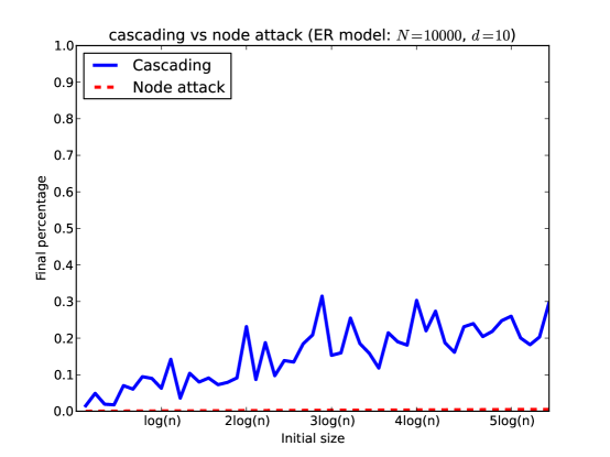
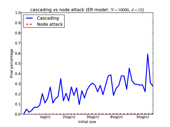
Figure 1: (a), (b) are the curves of fractions of sizes of infection sets and injury sets by attacks of the top degree nodes of small sizes, i.e., up to $5\log n$, for networks of the ER model for $n=10,000$ and for $d=10$ and $15$ respectively. The sizes of the infection sets are the largest ones among $100$ times attacks under random threshold cascading failure model. The infection sets and injury sets correspond to the blue and red curves respectively.

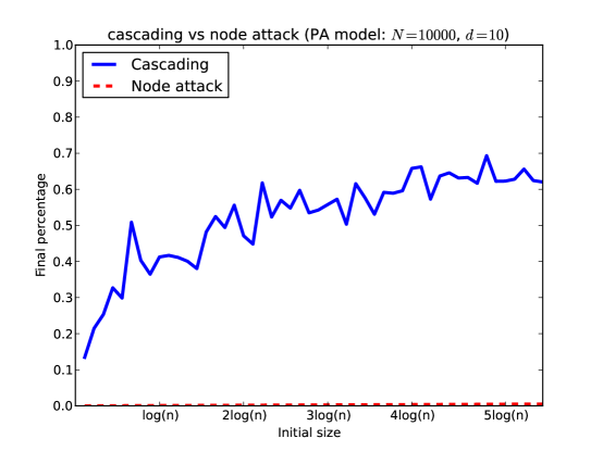
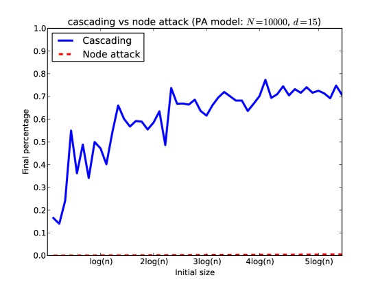
Figure 2: (a), (b) are the curves of fractions of sizes of infection sets and injury sets by attacks of the top degree nodes of small sizes, i.e., up to $5\log n$, for networks of the PA model for $n=10,000$ and for $d=10$ and $15$ respectively. The sizes of the infection sets are the largest ones among $100$ times attacks under random threshold cascading failure model. The infection sets and injury sets correspond to the blue and red curves respectively.

From Figures  1,  1,  2 and  2, we have that the main issue of network security is to resist the global failure of networks under cascading failure models, that for both theory and applications, it suffices to guarantee the security against attacks of sizes polynomial in $\log n$, and that topological structures of networks are essential to the security of the networks, observed from the comparison of infection fractions between the ER and the PA models.

According to the experiments in Figures  1,  1,  2 and  2, we propose the following hypotheses.

Security Hypothesis: We say that a network is secure, if any small number of attacks of any strategy will never cause a global failure of the network.

Robustness Hypothesis: We say that a network is robust, if a small number of random errors of the network will never cause a global failure of the network.

2 Definitions of security and robustness

As mentioned in Section 1, the main issue is the security for cascading failure models and for attacks of sizes polynomial in $\log n$.

We propose mathematical definitions for security and robustness of networks based on the security hypothesis and the robustness hypothesis summarized in Section 1, respectively.

We consider the security of networks with arbitrary sizes. We define the security and robustness of networks under the threshold cascading failure model as follows:

Let $n$ be the number of nodes of the network. We define

Security With probability $1-o(1)$, the following event occurs: For any initial set $S$ of size ${\rm poly}(\log n)$, $S$ will not cause a global cascading failure, that is, the size of the infection set of $S$ in $G$ is $o(n)$.

and

Robustness With probability $1-o(1)$, a small number, i.e., ${\rm poly}(\log n)$, of random choices of the initial set $S$ will not cause a global cascading failure, that is, the size of the infection set of $S$ in $G$ is $o(n)$.

Let $\mathcal{M}$ be a model of networks. We investigate the security of networks constructed from model $\mathcal{M}$. We define the security of networks for attacks of cascading failure with both random threshold and uniform threshold respectively. Suppose that $G$ is a network of $n$ nodes, constructed from model $\mathcal{M}$, for large $n$.

Definition 2.1

(Random threshold security) For the cascading failure model of random threshold, we say that $G$ is secure, if almost surely, meaning that with probability $1-o(1)$, the following holds:

for any set $S$ of size bounded by a polynomial of $\log n$, the size of the infection set (or cascading failure set) of $S$ in $G$ is $o(n)$.

Definition 2.2

(Uniform threshold security) For the cascading failure model of uniform threshold, we say that $G$ is secure, if almost surely, the following holds: for an arbitrarily small $\phi$, i.e., $\phi=o(1)$, for any set $S$ of size bounded by a polynomial of $\log n$, $S$ will not cause a global $\phi$-cascading failure, that is, the size of the infection set of $S$ in $G$, written by ${\rm inf}^{\phi}_{G}(S)$, is bounded by $o(n)$.

Definition 2.3

(Security of model $\mathcal{M}$) Let $\mathcal{M}$ be a model of networks. We say that model $\mathcal{M}$ is secure, if networks constructed from model $\mathcal{M}$ are secure for both random and uniform threshold cascading failure models of attacks.

Definition 2.4

(Random threshold robustness) For the cascading failure model of random threshold, we say that $G$ is robust, if almost surely, meaning that with probability $1-o(1)$, the following holds:

for randomly chosen set $S$ of size bounded by a polynomial of $\log n$, the size of the infection set of $S$ in $G$ is $o(n)$.

Definition 2.5

(Uniform threshold robustness) For the cascading failure model of uniform threshold, we say that $G$ is robust, if almost surely, the following holds: for an arbitrarily small $\phi$, i.e., $\phi=o(1)$, for randomly chosen set $S$ of size bounded by a polynomial of $\log n$, $S$ will not cause a global $\phi$-cascading failure, that is, the size of the infection set of $S$ in $G$, written by ${\rm inf}_{G}^{\phi}(S)$, is bounded by $o(n)$.

Definition 2.6

(Robustness of model $\mathcal{M}$) Let $\mathcal{M}$ be a model of networks. We say that model $\mathcal{M}$ is robust, if networks constructed from model $\mathcal{M}$ are robust for both random and uniform threshold cascading failure models of random errors.

In Definitions 2.1,  2.2,  2.4 and  2.5, the sizes of attacks or random errors are polynomial in $\log n$. This is sufficient for both theory and applications. The reason is that networks constructed from both the ER and PA models are insecure, in the sense that attacks of $O(\log n)$ top degree nodes may generate a constant fraction of nodes of the networks to be infected, as shown in Figures  1,  1,  2 and  2.

3 Security model of networks: algorithms and principles

From Figures  1,  1,  2 and  2, we know that nontrivial networks of both the ER model and the PA model are insecure. This poses fundamental questions such as: Are there networks with power law and small world property that are secure by Definitions 2.1 and 2.2? What mechanisms guarantee the security of networks? Is there any algorithm to construct secure networks?

In  (?), the authors proposed a security model of networks, and showed by experiments that networks of the security model are much more secure than that constructed from both the ER and PA models.

Definition 3.1

(Security model) Let $d\geq 4$ be a natural number and $a$ be a real number, which is called homophyly exponent. We construct a network by stages.

1. Let $G_{2}$ be an initial graph such that each node is associated with a distinct color, and called seed.

2. Let $i>2$. Suppose that $G_{i-1}$ has been defined. Define $p_{i}=(\log i)^{-a}$.

3. With probability $p_{i}$, $v$ chooses a new color, $c$ say. In this case, do:

   1. we say that $v$ is the seed node of color $c$,

   2. (Preferential attachment scheme) add an edge $(u,v)$, such that $u$ is chosen with probability proportional to the degrees of nodes in $G_{i-1}$, and

   3. (Randomness) add $d-1$ edges $(v,u_{j})$, $j=1,2,\ldots,d-1$, where $u_{j}$’s are chosen randomly and uniformly among all seed nodes in $G_{i-1}$.

4. (Homophyly and preferential attachment) Otherwise. Then $v$ chooses an old color, in which case, then:

   1. let $c$ be a color chosen randomly and uniformly among all colors in $G_{i-1}$,

   2. define the color of $v$ to be $c$ , and

   3. add $d$ edges $(v,u_{j})$, for $j=1,2,\ldots,d$, where $u_{j}$’s are chosen with probability proportional to the degrees of all the nodes that have the same color as $v$ in $G_{i-1}$.

It is clear that Definition 3.1 is a dynamic model of networks for which homophyly, randomness and preferential attachment are the underlying mechanisms.

As shown in  (?),   (?), networks constructed from the security model are much more secure than that of the ER and PA models. To understand the intuition of the security model, we use a figure in  (?), Figure 3 here. It depicts three curves of sizes of infection sets of attacks of top degree nodes of sizes up to $5\cdot\log n$ under random threshold cascading failure model on networks generated from the security model, the ER model and the PA model respectively. The curves correspond to the largest infection set among $100$ times of attacks over random choices of thresholds of the networks. The figure shows that networks of the security model are in deed much more secure than that of both the ER and the PA models, even if we just take the homophyly exponent $a>1$ in the security model.

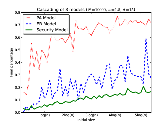
Figure 3: The curves are cascading failures of networks of the ER model, the PA model and the security model for $n=10,000$, $d=15$ and $a=1.5$

Experiments in  (?) showed the following properties:

1. The mechanisms of homophyly, randomness and preferential attachment ensure that networks of the security model satisfy a number of structural properties such as:

   1. (Small community phenomenon) A network, $G$ say, is rich in quality communities of small sizes.

      In fact, let $S$ be a homochromatic set of $G$. Then the induced subgraph of $S$, written by $G_{S}$, is highly connected, and the conductance of $S$, written by $\Phi(S)$, is bounded by a number reversely proportional to a constant power of the size of the community, i.e., less than or equal to, $O(\frac{1}{|S|^{\beta}})$, for some constant $\beta$, where $|S|$ is the size of $S$.

   2. (Internal centrality) Each community is the induced subgraph of nodes of the same color, which follows a preferential attachment, and hence has only a few nodes dominating the internal links of the community.

      This shows a remarkable local heterogeneity of the networks.

   3. (External centrality) Each community has a few nodes, including the seed of the community, which dominate the external links from the community to outside of the community.

2. (Power law) The networks follow a power law.

3. (Small world property) The networks have small diameters.

4. (Global Randomness and uniformity) There is a high degree of randomness and uniformity among the edges between nodes of different colors.

   This shows that the networks have a global homogeneity and a global randomness.

5. A non-seed node, $x$ in a community $G_{X}$, created at time step $t$ can be infected by a neighbor community $G_{Y}$, only if the seed node $y_{0}$ of $G_{Y}$ is created at a time step $s>t$ and an edge $(y_{0},x)$ is created by (3) (b) of Definition 3.1.

The structural properties in (1) above allow us to develop a methodology of community analysis of networks. (2) and (3) show that the networks constructed from the security model have the most important properties of usual networks. (4) and (5) ensure that infections among different communities are hard. This intuitively explains the reason why networks constructed from the security model show much better security than that of the classic ER and PA models.

The arguments above imply that the small community phenomenon, local heterogeneity, global homogeneity and global randomness are essential to the security of networks with power law and small world property.

In the present paper, we will show that the security model is provably secure by Definition 2.3. The key idea of the proofs is a merging of some principles of topology, probability and combinatorics.

We use $\mathcal{S}(n,a,d)$ to denote the set of random graphs of $n$ nodes constructed by the security model with homophyly exponent $a$ and average number of edges $d$ .

Let $G$ be a network constructed from the security model. We have that each node is assigned a color. This new dimension of colors allows us to characterize the structures of the networks. In our security model, every node has its own characteristics from the very beginning of its birth. This feature is remarkably different from the classic models such as the ER and the PA models. Anyway, the extra dimension of colors is essential to our understanding of security of networks.

We call a set of nodes of the same color, $\kappa$ say, a homochromatic set, written by $S_{\kappa}$.

We say that an edge is a local edge if two of its endpoints share the same color, and global edge, otherwise.

At first, we prove some structural properties of networks of the security model.

Theorem 3.1

(Fundamental theorem of the security model) Let $a>1$ be the homophyly exponent, and $d\geq 4$ be a natural number. Let $G=(V,E)$ be a network constructed by $\mathcal{S}(n,a,d)$.

Then with probability $1-o(1)$, the following properties hold:

1. (Basic properties):

   1. (Number of seed nodes is large) The number of seed nodes is bounded in the interval $[\frac{n}{2\log^{a}n},\frac{2n}{\log^{a}n}]$.

   2. (Communities whose vertices are interpretable by common features are small) Each homochromatic set has a size bounded by $O(\log^{a+1}n)$.

2. For degree distributions, we have:

   • (Internal centrality) The degrees of the induced subgraph of a homochromatic set follow a power law.

   • The degrees of nodes of a homochromatic set follow a power law.

   • (Power law) Degrees of nodes in $V$ follow a power law.

3. For node-to-node distances, we have:

   • (Local communication law) The induced subgraph of a homochromatic set has a diameter bounded by $O(\log\log n)$.

   • (Small world phenomenon) The average node to node distance of $G$ is bounded by $O(\log n)$.

   • (Local algorithm to find short path between two nodes) There is an algorithm to find a short path between arbitrarily given two nodes in time $O(\log n)$.

4. (Small community phenomenon) There are $1-o(1)$ fraction of nodes of $G$ each of which belongs to a homochromatic set, $W$ say, such that the size of $W$ is bounded by $O(\log^{a+1}n)$, and that the conductance of $W$, $\Phi(W)$, is bounded by $O\left(\frac{1}{|W|^{\beta}}\right)$ for $\beta=\frac{a-1}{4(a+1)}$.

   This shows that the network is rich in quality communities of small sizes.

Theorem 3.1 explores an interesting topology of a network $G$: (i) $G$ consists of a local structure and a global structure, (ii) the local structure of $G$ is determined by the small communities which have a number of local properties, and (iii) the global structure of $G$ follows its own laws. The network is rich in quality communities of small sizes which compose the interpretable local structures of the network. On the other hand, there is a global structure of the network which ensures that the whole network is highly connected, with a power law distribution, and a small diameter property. Communications in $G$ have two types, the first is the local communications within the small communities of length $O(\log\log n)$ and the second is the global ones which make the whole network to be highly connected of length $O(\log n)$. More importantly, there exists a local algorithm running in time $O(\log n)$ to navigate in the whole network. Most of the communications are local ones having length within $O(\log\log n)$, and the rest of communications are global ones with length bounded by $O(\log n)$. The construction of a network with explicit marks of local and global structures by Definition 3.1 allows local algorithms of time complex $O(\log n)$ to find useful information in the whole network. This suggests a new algorithmic problem, that is, to find network algorithms of time complexity polynomial in $\log n$ for finding useful information.

Theorem 3.1 ensures that all the communities are small. This guarantees that even if a single node in a small community infects the whole community, the cascading failure is still a local cost. However it is not intuitive to understand from Theorem 3.1 the reason why networks of the security model are secure. In fact, to prove the security theorems, we need to develop some probabilistic and combinatorial properties of the networks. In   (?), the authors analyzed experimentally some of these properties.

Suppose that $G=(V,E)$ is a network constructed from the security model. For a subset $X\subset V$, we always use $G_{X}$ to denote the induced subgraph of $X$ in $G$.

For a set of nodes $S$, we define $C(S)$ to be the set of colors that appear in $S$. For a node $v$, we use $N(v)$ to denote the set of neighbors of $v$. Given a node $v$, we define the length of degrees of $v$ to be the number of colors associated with the neighbors of $v$, i.e., $|C(N(v))|$, written by $l(v)$.

Suppose that $N_{1},N_{2},\cdots,N_{l}$ are all the neighbors of $v$ such that nodes in each $N_{i}$ share the same color, and that nodes in different $N_{i}$’s have different colors. Let $d_{i}$ be the size of $N_{i}$, for each $i\in\{1,2,\cdots,l\}$. Suppose that $d_{1}\geq d_{2}\geq\cdots\geq d_{l(v)}$ (ties break arbitrarily). In this case, we say that $d_{i}$ is the $i$-th degree of $v$, and the color of nodes in $N_{i}$ is the $i$-th color of neighbors of $v$, for all $i\in\{1,2,\cdots,l\}$.

The length of degrees, the $i$-th degree and the $i$-th color of neighbors of vertices have some interesting properties, including the ones validated by experiments in   (?): (i) The length of degrees of a vertex is always bounded by $O(\log n)$, (ii) The first degrees $d_{1}$’s are large, (iii) The second degrees are always as small as constants, and (iv) For a vertex $v$, if the length of degrees of $v$ is $l(v)>1$, then for any $i>1$, the $i$-th color of neighbors of $v$ is distributed with a high degree of randomness and uniformity. These properties are essential to the experimental analysis of security of the networks in  (?).

To theoretically prove the results, we define some useful notations.

Definition 3.2

Let $G=(V,E)$ be a network constructed from the security model. Given a node $v\in V$:

1. For every $j$, we define the $j$-th degree of $v$ at the end of time step $t$ to be the number of the $j$-th largest set of homochromatic neighbors at the end of time step $t$, written by $d_{j}(v)[t]$.

2. We define the $j$-th degree of $v$ to be the $j$-th degree of $v$ at the end of the construction of network $G$, written by $d_{j}(v)$.

3. We define the length of degrees of $v$ at the end of time step $t$ to be the number of colors associated with neighbors of $v$ at the end of time step $t$, written by $l(v)[t]$.

4. We define the length of degrees of $v$ to be the length of degrees of $v$ at the end of the construction of $G$, written by $l(v)$.

In sharp contrast to classic graph theory, for a network constructed from our security model, $G$ say, and a vertex $v$ of $G$, $v$ has a priority of degrees. This new feature must be universal in real networks in the following sense: A community is an interpretable object in a network such that nodes of the same community share common features. In this case, a vertex $v$ may have its own community and may link to some neighbor communities by some priority ordering. In our model, a node $v$ more likes to contact with nodes sharing the same color (or feature) with it, and has no much preferences in contacting with nodes in its neighbor communities.

Definition 3.3

(Degree Priority) Let $v$ be a node of $G$ constructed from the security model created at time step $t_{0}$, and $t\geq t_{0}$.

1. Suppose that $N_{1},N_{2},\cdots,N_{l}$ are all the homochromatic neighbors of $v$ at the end of time step $t$ listed decreasingly by the sizes of the sets $N_{j}$. For $d_{j}=|N_{j}|$ for each $j$, we say that $(d_{1},d_{2},\cdots,d_{l})$ is the degree priority of $v$ at the end of time step $t$, written by $dp(v)[t]=(d_{1},d_{2},\cdots,d_{l})$.

2. We define the degree priority of $v$ in $G$ to be the degree priority of $v$ at the end of the construction of $G$, written by $dp(v)$.

The degree priority of nodes in $G$ satisfies some nice probabilistic and combinatorial properties.

Theorem 3.2

(Degree Priority Theorem) Let $G$ be a network constructed from the security model with $d\geq 2$, and $a>1$. Then with probability $1-o(1)$, for a randomly chosen node $v$, the following properties hold:

1. The length of degrees of $v$ is bounded by $O(\log n)$, which is an upper bound independent of $a$.

2. The first degree of $v$ is the number of neighbors that share the same color as $v$.

3. The second degree of $v$ is bounded by $O(1)$, so that for any possible $j>1$, the $j$-th degree of $v$ is $O(1)$.

4. The first degree of a seed node is lower bounded by $\Omega(\log^{\frac{a+1}{4}}n)$.

By (2), (3) and (4) of Theorem 3.2, we understand that for a community $G_{X}$ induced by a homochromatic set $X$, the seed node, $x_{0}$ say, of $X$ has a large first degree and constant second degree, so that it is unlikely to be infected by a single neighbor community, $G_{Y}$ say. Combining with (1), this ensures that for properly chosen $a$, the seed node $x_{0}$ of $G_{X}$ is hard to be infected by the collection of all its neighbor communities alone. Such a community is regarded as a strong community. Theorem 3.1 ensures that for properly chosen $a$, almost all communities are strong, so that each of them is hard to be infected by the collection of all its neighbor communities alone.

Combining Theorem 3.1 and Theorem 3.2 gives us a better understanding for the reasons why networks of the security model are secure. However, to prove the security theorems, we have to understand the cascading behaviors of attacks in the networks.

We define a community of $G$ is the induced subgraph of a homochromatic set. We say that a community, $G_{X}$ say, is created at time step $t$ if the seed node $x_{0}$ of $X$ is created at time step $t$.

To understand the cascading behaviors, we define:

Definition 3.4

Let $x$ and $y$ be two nodes of $G$. We say that $x$ injures $y$, if the infection of $x$ contributes to the probability that $y$ becomes infected. Otherwise, we say that $x$ fails to injure $y$.

We will show that the infection of a community from a neighbor community satisfies a number of combinatorial properties.

Theorem 3.3

(Infection-Inclusion Theorem) Suppose that $X$ and $Y$ are two homochromatic sets, and that $G_{X}$ and $G_{Y}$ are two communities. Let $x_{0}$, and $y_{0}$ be the seed nodes of $X$ and $Y$ respectively. Suppose that $x_{0}$ and $y_{0}$ are created at time step $s$ and $t$ respectively. Then the injury of $G_{Y}$ from community $G_{X}$ satisfies the following properties:

1. If $s<t$, then

   1. The community $G_{X}$ created at time step $s$ fails to injure any non-seed node in the community $G_{Y}$ created at time step $t$.

   2. The injury of the seed node $y_{0}$ created at time step $t$ from the whole community created at time step $s$ is bounded by a constant $O(1)$.

2. If $s>t$, then

   1. All the non-seed nodes in $G_{X}$ created at time step $s$ fail to injure any node in the community $G_{Y}$ created at time step $t$.

   2. The injury of the seed node created at time step $t$ from the community created at time step $s$ is bounded by $1$.

   3. The injury of a non-seed node in the community created at time step $t$ from the seed node created at time step $s$ follows the edge created by step (3) (b) of Definition 3.1.

3. The seed node $y_{0}$ of $G_{Y}$ created at time step $t$ can be injured only by:

   1. Communities created at time step $<t$.

   2. The seed nodes of communities created at time step $>t$.

4. A non-seed node $y$ of $G_{Y}$ created at time step $t$ can be injured only by seed nodes created at time step $>t$ through the edge created by (3) (b) of Definition 3.1.

(1), (2) and (3) of Theorem 3.3, together with Theorem 3.2, show furthermore that, a seed node, $v$ say, of $G$ are strong against infections from the collection of all the communities other than its own community.

Suppose that $X$, $Y$ and $X$ are three homochromatic sets created at time steps $t_{1}$, $t_{2}$ and $t_{3}$ respectively. Let $x_{0}$, $y_{0}$ and $z_{0}$ be the seed nodes of $X$, $Y$ and $Z$ respectively. It is possible that $x_{0}$ infects a non-seed node $y_{1}$ of $Y$, $y_{1}$ infects all nodes in $Y$, including $y_{0}$, and $y_{0}$ infects a non-seed node $z_{1}$ of $Z$. (4) of Theorem 3.3 ensures that $t_{1}>t_{2}>t_{3}$, and that the edges $(x_{0},y_{1})$ and $(y_{0},z_{1})$ must be created by (3) (b) of Definition 3.1. The key point is that the edges $(x_{0},y_{1})$ and $(y_{0},z_{1})$ must be embedded in a tree of height $O(\log n)$ which we will call the infection priority tree (IPT, for short) $T$ of $G$. The infection priority tree $T$ of $G$ is essentially a graph constructed by the preferential attachment model with average number of edges $d^{\prime}=1$, which almost surely has height $O(\log n)$.

Therefore a targeted or infected strong community triggers at most $O(\log n)$ many strong communities to be infected, by Theorem 3.1, each community has size at most $O(\log^{a+1}n)$. For any initial set of attacks $S$ of size polynomial in $\log n$, suppose that every community which is not strong has already been infected by attacks on $S$ automatically. Let $K$ be the number of communities that are not strong. Then there are at most $|S|+K$ strong communities trigger infections in the infection priority tree $T$. This shows that there are at most $O((|S|+K)\cdot\log n)$ communities in each of which there is at least one node is infected by attacks on $S$. In this case, again by Theorem 3.1, even if all the nodes in an infected community are infected, the total number of infected nodes is a negligible number comparing with the size of the network. This sketch depends on an estimation of $K$, the number of communities that are not strong, which will be given in the full proofs in later sections.

Therefore (1), (2) and (4) of Theorem 3.3 ensure that the infection of a non-seed node, $v$ say, is always one-way from a seed node created late than $v$, following an edge in the infection priority tree. By modulo the injury among the seed nodes, we are able to show that the infections of non-seed nodes can only proceed in the infection priority tree of height $O(\log n)$.

Now we fully understand that the combination of Theorems 3.1, 3.2, and 3.3 does allow us to prove some security theorems of the security model. This also explores the following security principle of networks.

Security Principle:

1. Small community phenomenon (by Theorem 3.1)

2. The number of seed nodes or hubs is large (by Theorem 3.1)

3. Almost all seed nodes (or hubs) are strong against infections from the collection of all their neighbor communities alone (by Theorem 3.2)

4. There exists an infection priority tree $T$ of $G$ such that infection of non-seed nodes of a community from a neighbor community can only be triggered by seed nodes of the neighbor community through edges in the infection priority tree $T$ of $G$ (by Theorem 3.3)

5. The infection priority tree $T$ of $G$ has height $O(\log n)$ (to be proved in Subsection 7.1)

4 Security Theorems

In this section, we state the theorems and discuss the relationships among the theorems.

By applying Theorems 3.1, 3.2 and 3.3, we are able to prove that networks constructed from the security model are secure against any attacks of small sizes under both uniform and random threshold cascading failure models.

For the uniform threshold cascading failure model, we have:

Theorem 4.1

(Uniform threshold security theorem) Let $G$ be a graph constructed from $\mathcal{S}(n,a,d)$ with $p_{i}=\log^{-a}i$ for homophyly exponent $a>4$ and for $d\geq 4$. Let the threshold parameter $\phi=O\left(\frac{1}{\log^{b}n}\right)$ for $b=\frac{a}{2}-2-\epsilon$ for arbitrarily small $\epsilon>0$.

Then with probability $1-o(1)$ (over the construction of $G$), there is no initial set of poly-logarithmic size which causes a cascading failure set of non-negligible size. Precisely, we have that for any constant $c>0$,

$$\Pr_{{}G\in_{\rm R}\mathcal{S}(n,a,d),\ G=(V,E)}\left[\forall S\subseteq V,\ |S|=\lceil\log^{c}n\rceil,\ |{\rm inf}_{G}^{\phi}(S)|=o(n)\right]=1-o(1),$$

where ${\rm inf}_{G}^{\phi}(S)$ is the infection set of $S$ in $G$ with uniform threshold $\phi$.

By Theorem 4.1, if $a>4$, and $d\geq 4$, then for $\phi=O(1/\sqrt{\log^{b}n})$, networks constructed by the security model $\mathcal{S}(n,a,d)$ are $\phi$-secure. Here $\phi$ is arbitrarily close to $0$, i.e., $\phi=o(1)$. Therefore, by Definition 2.2, for $a>4$, and $d\geq 4$, networks in $\mathcal{S}(n,a,d)$ are secure under the uniform threshold cascading failure model of attacks.

For the random threshold cascading failure model, each node $v$ picks randomly, uniformly and independently a threshold $\rho_{v}$ from $1,2,\ldots,d_{v}$. Let ${\rm inf}_{G}^{\rm R}(S)$ be the infection set of attacks on $S$ in $G$. We show that graphs generated by $\mathcal{S}(n,a,d)$ are secure.

Theorem 4.2

(Random threshold security theorem ) Let $a>6$ be the homophyly exponent, and $d\geq 4$. Suppose that $G$ is a graph generated from $\mathcal{S}(n,a,d)$.

Then with probability $1-o(1)$ (over the construction of $G$), there is no initial set of poly-logarithmic size which causes a cascading failure set of non-negligible size. Formally, we have that for any constant $c>0$,

$$\Pr_{{}G\in_{\rm R}\mathcal{S}(n,a,d),\ G=(V,E)}\left[\forall S\subseteq V,|S|=\lceil\log^{c}n\rceil,|{\rm inf}_{G}^{\rm R}(S)|=o(n)\right]=1-o(1).$$

Theorems 4.1 and  4.2 show that for appropriately chosen parameters, networks constructed from the security model are provably secure for any attacks of small sizes under both uniform and random threshold cascading failure models. By Definitions 2.2, 2.1,  2.3, and by Theorems 4.1 and  4.2, the security model in Definition 3.1 is secure.

The preferential attachment model was proposed to capture real networks. It has become a classic model of networks. We use $\mathcal{P}(n,d)$ to denote the set of random graphs of $n$ nodes constructed from the PA model with average number of edges $d$. Numerous experiments have shown that networks of the preferential attachment model are insecure, see for instance Figure 3. Therefore the best possible result we could look for would be the robustness results for the PA model. People may take for granted that networks of the PA model are robust, although there was no definition for robustness in the literature. Here we have rigorous definition of robustness of a model of networks, given in Definitions 2.5, 2.4, and 2.6. This poses a fundamental question: Are networks of the PA model really robust?

We show that, for large enough edge parameter $d$, for uniform threshold cascading failure model, if the threshold is slightly less than $1/d$, then just one randomly picked initial node is sufficient to infect a significant fraction of the whole network with high probability.

Theorem 4.3

(Global cascading of a single node in PA) For any $\varepsilon>0$, there exists a positive integer $d_{\varepsilon}$ such that for any integer $d\geq d_{\varepsilon}$, if $G=(V,E)$ is constructed from $\mathcal{P}(n,d)$, then with probability $1-o(1)$ (over the construction of $G$), the following inequality holds:

$$\Pr\limits_{v\in_{\rm R}V}[{\rm inf}_{G}^{\phi}(\{v\})=V]\geq\frac{2}{3}\left(1-\frac{1}{(1+\varepsilon)^{2}}\right),$$

where $\phi=\frac{1}{(1+\varepsilon)d}$.

Therefore if $\log n$ initial nodes are randomly picked, then the whole graph $G$ will be infected with probability $1-o(1)$.

Theorem 4.4

(Global cascading theorem of PA) For any $\varepsilon>0$, there exists a positive integer $d_{\varepsilon}$ such that for any integer $d\geq d_{\varepsilon}$, for threshold parameter $\phi=\frac{1}{(1+\varepsilon)d}$,

$$\Pr_{{}S\subset_{\rm R}V,\ |S|=\log n}[{\rm inf}_{G}^{\phi}(\{S\})=V]=1-o(1).$$

Proof 1

By Theorem 4.3.

Consequently, $\mathcal{P}(n,d)$ is not $\phi$-robust for all $\phi\leq\frac{1}{(1+\varepsilon)d}$. By Definitions 2.5 and 2.6, and by Theorem 4.4, the preferential attachment model is not robust. In fact, each of the nontrivial networks constructed from the PA model is non-robust. This result shows that if real networks truthfully follow the PA model, then the networks would be not only insecure, but also unavoidably non-robust. This makes the situation even worse in practical applications, because, a few or even one random error may cause a global cascading failure of the whole network.

On the other hand, we also show that if the threshold is larger than $1/d$, then with probability $1-o(1)$, $o(\sqrt{n})$ randomly picked initially infected nodes are insufficient to infect even one more node, and the PA model is robust in this case. In fact, we are able to prove a stronger result that holds for arbitrarily given simple (or almost simple) graphs .

Theorem 4.5

(Robustness theorem of graphs) Given a simple graph $G=(V,E)$ whose nodes have minimum degree $d$. Let $n=|V|$ and $d$ be a constant independent of $n$. Let $\phi>\frac{l}{d}$, where $l$ is an integer from the interval $[1,d-1]$. Let $S\subseteq V$ be a randomly picked subset of size $k=o(n^{\frac{l}{l+1}})$. Then

$$\Pr\limits_{S\subset_{\rm R}V}[{\rm inf}_{G}^{\phi}(S)=S]=1-o(1).$$

By using this, we have:

Theorem 4.6

(Robustness theorem of PA) For any integer $d\geq 2$ and $\phi>\frac{1}{d}$, $\mathcal{P}(n,d)$ is $\phi$-robust.

Proof 2

Since the number of multi-edges and self-loops in $\mathcal{P}(n,d)$ is at most $O(\log n/n)$ (with probability almost $1$), the probability that, in randomly picked $n^{\lambda}$ ($\lambda\leq 1/2$) nodes, there is a node associating to some multi-edge or self-loop is upper bounded by $o(1)$. It is easily observed that the result is a straightforward corollary of Theorem 4.5 in the case of $l=1$.

Theorem 4.6 implies that for a network constructed from the PA model, if every node has a threshold $\geq\phi$ for some large constant $\phi$, then the network is robust against random errors ( of small sizes).

By Theorems  4.4 and  4.6, the value $1/d$ is a key threshold for the robustness of the PA model. The two theorems characterize the robustness of networks of the PA model under uniform threshold cascading failure model, leaving open for the case of $\phi=1/d$. This clarifies the experimental results of robustness of networks of the PA model.

The remaining sections are devoted to proofs of Theorems 3.1, 3.2, 3.3,  4.1,  4.2,  4.3 and 4.5. In section  5, we prove Theorem  3.1. In Section 6, we prove Theorems 3.2 and 3.3. In Section  7, we prove Theorems 4.1, and  4.2 by using Theorems 3.1,  3.2 and 3.3. In Section  8, we prove the threshold theorem of robustness of networks of the PA model, consisting of Theorems  4.3 and  4.5. In Section 9, we extend the security model to high dimensions so that a node has $k$ colors for $k>1$. In this case, communities in the network are overlapping. We show that overlapping communities undermine security of networks. In Section 10, we summarize the conclusions and discuss some future directions.

5 The Fundamental Theorem of the Security Model

In this section, we prove Theorem  3.1. Before proving the theorem, we state the Chernoff bound below which will be frequently used in our proofs.

Lemma 5.1

(Chernoff bound,  (?)) Let $X_{1},\ldots,X_{n}$ be independent random variables with $\Pr[X_{i}=1]=p_{i}$ and $\Pr[X_{i}=0]=1-p_{i}$. Denote the sum by $X=\sum_{i=1}^{n}X_{i}$ with expectation $E(X)=\sum_{i=1}^{n}p_{i}$. Then we have

$$\Pr[X\leq E(X)-\lambda]\leq\exp\left(-\frac{\lambda^{2}}{2E(X)}\right),$$

$$\Pr[X\geq E(X)+\lambda]\leq\exp\left(-\frac{\lambda^{2}}{2(E(X)+\lambda/3)}\right).$$

Let $G$ be a network constructed from the security model. We now prove Theorem  3.1. We will prove (1), (2), (3) and (4) of Theorem 3.1 in Subsections 5.1, 5.2, 5.3 and 5.4 respectively.

5.1 Basic Properties

In this subsection, we prove (1) of Theorem  3.1. It consists of two results, the first is the estimation of number of seed nodes, and the second is the upper bound of sizes of the homochromatic sets.

Proof 3

(Proof of (1) of Theorem  3.1) We use $G[t]$ to denote the graph constructed at the end of time step $t$ of the construction of $G$. Let $T_{1}=\log^{a+1}n$, and $C_{t}$ be the set of all colors appear in $G[t]$.

For (i). It suffices to show that the size of $C_{t}$ is bounded as desired. For this, we have:

Lemma 5.2

With probability $1-o(1)$, for all $t\geq T_{1}$, $\frac{t}{2\log^{a}t}\leq|C_{t}|\leq\frac{2t}{\log^{a}t}$.

Proof 4

The expectation of $|C_{t}|$ is

$$E[|C_{t}|]=2+\sum_{i=3}^{t}\frac{1}{\log^{a}i}.$$

By indefinite integral

$$\int(\frac{1}{\log^{a}x}-\frac{a}{\log^{a+1}x})dx=\frac{x}{\log^{a}x}+C,$$

we know that if $t$ is large enough, then

$$\sum_{i=3}^{t}\frac{1}{\log^{a}i} \leq 1+\int_{2}^{t}\frac{1}{\log^{a}x}dx$$

$$\leq \int_{2}^{t}\frac{6}{5}(\frac{1}{\log^{a}x}-\frac{a}{\log^{a+1}x})dx$$

$$\leq \frac{4t}{3\log^{a}t},$$

where $\frac{6}{5}$ and $\frac{4}{3}$ are chosen arbitrarily among the numbers larger than $1$. Similarly,

$$\sum_{i=3}^{t}\frac{1}{\log^{a}i} \geq \int_{2}^{t}\frac{1}{\log^{a}x}dx$$

$$\geq \int_{2}^{t}\frac{5}{6}(\frac{1}{\log^{a}x}-\frac{a}{\log^{a+1}x})dx$$

$$\geq \frac{3t}{4\log^{a}t}.$$

By the Chernoff bound and the fact that $t\geq T_{1}=(\log n)^{a+1}$, with probability $1-exp(-\Omega(\frac{t}{\log^{a}t}))=1-o(n^{-1})$, we have $\frac{t}{2\log^{a}t}\leq|C_{t}|\leq\frac{2t}{\log^{a}t}$. By the union bound, such an inequality holds for all $t\geq T_{1}$ with probability $1-o(1)$.

(i) follows from Lemma 5.2.

Lemma 5.2 depends on only the probability $p_{i}=1/(\log i)^{a}$ with which the node created at time step $i$ chooses a new color. It is a useful fact throughout the proofs, from which we define:

Definition 5.1

We define $\mathcal{E}$ to be the event that $|C_{t}|$ is bounded in the interval $\left[\frac{t}{2\log^{a}t},\frac{2t}{\log^{a}t}\right]$.

By Lemma 5.2, almost surely, the event $\mathcal{E}$ holds for all $t\geq T_{1}$.

For (ii). We estimate the size of all the homochromatic sets.

Lemma 5.3

With probability $1-o(1)$, the following properties hold:

(1) Every community has size bounded by $O(\log^{a+1}n)$, and

(2) For every $t\geq T_{1}$, every community at the end of time step $t$ has size bounded by $O(\log^{a+1}t)$.

Proof 5

For (1). It suffices to show that with probability $1-o(n^{-1})$, the homochromatic set of the first color $\kappa$ has size $O(\log^{a+1}n)$.

We define an indicator random variable $Y_{t}$ for the event that the vertex created at time $t$ chooses color $\kappa$. We also define $\{Z_{t}\}$ to be the independent Bernoulli trails such that

$$\Pr[Z_{t}=1]=\left(1-\frac{1}{\log^{a}n}\right)\frac{2\log^{a}t}{t}.$$

Conditioned on the event $\mathcal{E}$, we know that $Y:=\sum_{t=1}^{n}Y_{t}$ is stochastically dominated by $Z:=\sum_{t=1}^{n}Z_{t}$. The latter has an expectation

$$E[Z]\leq\sum_{t=1}^{n}\frac{2\log^{a}t}{t}\leq 2\log^{a+1}n.$$

By the Chernoff bound,

$$\Pr[Z>4\log^{a+1}n]\leq n^{-1}.$$

Therefore, with probability $1-n^{-1}$, the size of $S_{\kappa}$ is $Y\leq 4\log^{a+1}n$. (1) follows.

For (2). This follows from the proof of (1) above. (2) holds.

Lemma 5.3 follows.

(ii) holds.

This proves (1) of Theorem 3.1.

5.2 Power Law

In this subsection, we probe (2) of Theorem 3.1, consisting of power law of the induced subgraph of communities, of the degree distributions of the homochromatic sets, and of the whole network $G$.

Before proving the results, we first prove both a lower bound and an upper bound for the sizes of well-evolved communities.

Recall that $T_{1}=\log^{a+1}n$. Let $T_{2}=(1-\delta_{1})n$, for $\delta_{1}=\frac{10}{\log^{a-1}n}$. We have:

Lemma 5.4

With probability $1-o(1)$, both (1) and (2) below hold in $G$:

1. For a community created at a time step $\leq T_{2}$, it has size at least $\log n$;

2. For a community created at a time step $>T_{2}$, it has size at most $30\log n$.

Proof 6

For (1). We only need to prove that, on the condition of event $\mathcal{E}$ in Definition 5.1, any homochromatic set $S_{\kappa}$ created before time step $T_{2}+1$ has size at least $\log n$ with probability $1-o(n^{-1})$.

For every $t>T_{2}$, let $Y_{t}$ be the indicator random variable that the vertex, $v$ say, created at time step $t$ chooses old color $\kappa$. For $t>T_{2}$, let $\{Z_{t}\}$ be the independent Bernoulli trails such that

$$\Pr[Z_{t}=1]=(1-\frac{1}{\log^{a}(1-\delta_{1})n})\frac{\log^{a}t}{2t}.$$ (1)

Conditioned on the event $\mathcal{E}$, we know that $Y:=\sum_{t\geq T_{2}+1}^{n}Y_{t}$ stochastically dominates $Z:=\sum_{t\geq T_{1}+1}^{n}Z_{t}$, which has expectation

$$E[Z]\geq\sum_{t=T_{2}+1}^{n}\frac{\log^{a}t}{2t}\geq\frac{\delta_{1}}{2}\log^{a}(1-\delta_{1})n\geq 4\log n.$$

By the Chernoff bound,

$$\Pr[Z<\log n]\leq e^{-\frac{3^{2}\log n}{2\times 4}}=n^{-\frac{9}{8}}.$$

Thus, with probability $1-o(n^{-1})$, the size of $S_{\kappa}$ is at least $\log n$.

For (2). The proof is similar to that of (1) above. We only need to prove that, on the condition of event $\mathcal{E}$, any homochromatic set $S_{\kappa}$ created after $T_{2}$ has size at most $30\log n$ with probability $1-o(n^{-1})$. For $t>T_{2}$, we consider the Bernoulli random variables $\{Z_{t}\}$ defined by

$$\Pr[Z_{t}=1]=(1-\frac{1}{\log^{a}n})\frac{2\log^{a}t}{t}.$$ (2)

Note that

$$E[Z]\leq\sum_{t=T_{2}+1}^{n}\frac{2\log^{a}t}{t}\leq\frac{2\delta_{1}}{1-\delta_{1}}\log^{a}n.$$

By a similar analysis to that in (1) above, we know that with probability $1-o(n^{-1})$, the size of $S_{\kappa}$ is at most $30\log n$.

The proof of Lemma 5.4 depends on both the probability $1-p_{i}$ with which the newly created node chooses an old color, and the randomness and uniformity of the choice of the old color at time step $i$ for all $i$’s.

By Lemma 5.4, we know that each of the communities born before time step $T_{2}+1$ has expected size $\omega(1)$, and that all the communities born at time steps $\leq T_{2}$ account for ($1-o(1)$) of all the communities. Therefore we prove the power law distribution only for the communities born at time steps $\leq T_{2}$.

For both (i) and (ii). Now we turn to prove two results:

1. For each homochromatic set $X$, the degrees of nodes in $X$ follow a power law, and

2. For each homochromatic set $X$, the induced subgraph $G_{X}$ of $X$ follow a power law.

We prove both (A) and (B) together. We consider only the non-trivial homochromatic sets, i.e., the well-evolved communities, by ignoring the few most recently created communities.

By (4) of Definition 3.1, each community basically follows the classical preferential attachment model, we are able to give explicit expressions for the expected numbers of nodes of degree $k$ for all $k$, for each of the homochromatic sets and for the induced subgraphs of the homochromatic sets.

In fact, as we will show below that the contribution to the degrees of a homochromatic set from the global edges is much more smaller than that from the local edges of the homochromatic set. This is the key point to our proofs of the power law of almost all the communities.

We use $X$ to denote a homochromatic set of a fixed color, $\kappa$ say. Let $T_{0}$ be the time step at which $X$ is created.

For positive integers $s$ and $k$, we define $A_{s,k}$ to be the number of nodes of degree $k$ in $X$ when $|X|$ reaches $s$, $B_{s,k}$ to be the number of nodes of degree $k$ in the induced subgraph of $X$ when $|X|$ reaches $s$, and $g_{s,k}$ to be the number of global edges associated with the nodes in $X$ of degree $k$ in the induced subgraph of $X$ when $|X|$ reaches $s$. By definition, we have $A_{1,d}=1$ and $A_{1,k}=0$ for all $k>d$, and $B_{1,k}=0$ for all $k$. We also have $A_{s,k}=B_{s,k}+g_{s,k}$. Then we establish the recurrence formula for the expectations of both $A_{s,k}$ and $B_{s,k}$.

Firstly, we define some notations associated with $X$ and its size $|X|$:

– we use $T(s)$ (or $T$, for simplicity) to denote the time step at which the size of $X$ becomes to be $s$,

– we use $s_{1}$ to denote the number of global edges connecting to $X$ in the case that $|X|=s$.

We consider the time interval $(T(s-1),T(s))$. Then the number of times that a global edge is created and linked to a node in $X$ of degree $k$ at some time step in the interval $(T(s-1),T(s))$ is expected to be $\Theta(\frac{1}{\log^{a}T}\cdot\frac{k\cdot A_{s,k}}{2dT}/\frac{\log^{a}T}{T})=\Theta(\frac{k\cdot A_{s,k}}{\log^{2a}T})$. Denote $\Theta(\log^{2a}T)$ by $s_{2}$.

Then for $s>1$ and $k>d$, we have

$$E(A_{s,k})=A_{s-1,k}\left(1-\frac{kd}{2d(s-1)+s_{1}}-\frac{k}{s_{2}}\right)+A_{s-1,k-1}\cdot\left(\frac{(k-1)d}{2d(s-1)+s_{1}}+\frac{k-1}{s_{2}}\right)+O\left(\frac{1}{s^{2}}\right).$$

Taking expectations on both sides, we have

$$E(A_{s,k}) = E(A_{s-1,k})\left(1-\left(\frac{1}{2(s-1)+s_{1}/d}-\frac{1}{s_{2}}\right)k\right)$$ (3)

$$+E(A_{s-1,k-1})\left(\frac{1}{2(s-1)+s_{1}/d}+\frac{1}{s_{2}}\right)(k-1)+O\left(\frac{1}{s^{2}}\right).$$

If $k=d$, then

$$E(A_{s,d})=E(A_{s-1,d})\left(1-\left(\frac{1}{2(s-1)+s_{1}/d}-\frac{1}{s_{2}}\right)d\right)+1+O\left(\frac{1}{s^{2}}\right).$$ (4)

Similarly, for $s>1$ and $k>d$,

$$E(B_{s,k})=B_{s-1,k}-\frac{d\cdot(kB_{s-1,k}+g_{s-1,k})}{2d(s-1)+s_{1}}+\frac{d\cdot((k-1)B_{s-1,k-1}+g_{s-1,k-1})}{2d(s-1)+t_{1}}+O(\frac{1}{s^{2}}).$$

Taking expectations on both sides, we have

$$E(B_{s,k}) = E(B_{s-1,k})\left(1-\frac{kd}{2d(s-1)+s_{1}}\right)+E(B_{s-1,k-1})\cdot\frac{(k-1)d}{2d(s-1)+s_{1}}$$ (5)

$$+\frac{E(g_{s-1,k-1}-g_{s-1,k})}{2d(s-1)+s_{1}}+O(\frac{1}{s^{2}}).$$

If $k=d$, then

$$E(B_{s,d}) = B_{s-1,d}-\frac{d\cdot(dB_{s-1,d}+g_{s-1,d})}{2d(s-1)+s_{1}}+1+O(\frac{1}{s^{2}})$$ (6)

$$= B_{s-1,d}\left(1-\frac{d}{2(s-1)+s_{1}/d}\right)+\left(1-\frac{g_{s-1,d}}{2d(s-1)+s_{1}}\right),$$

and

$$E(B_{s,d})=E(B_{s-1,d})\left(1-\frac{d}{2(s-1)+s_{1}/d}\right)+\left(1-\frac{E(g_{s-1,d})}{2d(s-1)+s_{1}}\right).$$

To solve the recurrences, we invoke the following lemma.

Lemma 5.5

( (?), Lemma 3.1) Suppose that a sequence $\{a_{s}\}$ satisfies the recurrence relation

$$a_{s+1}=(1-\frac{b_{s}}{s+s_{1}})a_{s}+c_{s}~{}~{}{\it for}~{}~{}s\geq s_{0},$$

where the sequences $\{b_{s}\},\{c_{s}\}$ satisfy $\lim_{s\rightarrow\infty}b_{s}=b>0$ and $\lim_{s\rightarrow\infty}c_{s}=c$ respectively. Then the limitation of $\frac{a_{s}}{s}$ exists and

$$\lim_{s\rightarrow\infty}\frac{a_{s}}{s}=\frac{c}{1+b}.$$

For the recurrence of $E(A_{s,k})$, by Lemma 5.4, as $n$ goes to infinity, $t=\omega(1)$ also goes to infinity. By the definition of $s_{2}$, $s_{2}=\Theta(\log^{2a}T)=\omega(s)$.

To deal with $s_{1}$, we give a upper bound for the expected volume of $X$ at time $T$, denoted by $V_{T}$, as follows.

$$E(V_{T}) \leq \sum\limits_{i=2}^{T}\left[\left(1-\frac{1}{\log^{a}i}\right)\cdot\frac{2d}{|C_{i}|}+\frac{1}{\log^{a}i}\cdot\frac{dV_{i-1}}{2di}\right]$$

$$\leq \sum\limits_{i=2}^{T}\frac{2d}{|C_{i}|}=O\left(\sum\limits_{i=2}^{T}\frac{4d\log^{a}i}{i}\right)=O(\log^{a}T).$$

So it is easy to observe that $\frac{s_{1}}{t}=O\left(\frac{1}{\log^{a}T}\cdot\frac{V_{T}}{2dT}/\frac{\log^{a}T}{T}\right)=O\left(\frac{1}{\log^{a-1}T}\right)$ goes to zero as $s$ approaches to infinity.

For the recurrence of $E(B_{s,k})$, we show that as $s$ goes to infinity, both $\frac{E(g_{s-1,k-1}-g_{s-1,k})}{2d(s-1)+s_{1}}$ and $\frac{E(g_{s-1,d})}{2d(s-1)+s_{1}}$ approach to $0$. Define $g_{s}=\sum_{i}g_{s,i}$ to be the total number of global edges associated to $X$ when $|X|$ reaches $s$. We only have to show that $E(\frac{g_{s}}{s})\rightarrow 0$ as $s\rightarrow\infty$.

Suppose that the seed node of $X$ is created at time $T_{0}$.

$$E(g_{s})=O\left(\sum\limits_{i=T_{0}}^{T(s)}\frac{1}{\log^{a}i}\cdot\frac{V_{i}}{2di}\right)=O\left(\sum\limits_{i=T_{0}}^{T(s)}\frac{\log i}{2di}\right)=O(\log^{2}T(s)-\log^{2}T_{0}).$$

Note that when we consider the size of $X$ at sometime $t>T_{0}$, we have

$$E(|X|) = \sum\limits_{i=T_{0}}^{t}\left(1-\frac{1}{\log^{a}i}\cdot\frac{1}{|C_{i}|}\right)=\Omega\left(\sum\limits_{i=T_{0}}^{t}\frac{\log^{a}i}{2i}\right)$$

$$= \Omega\left(\int_{T_{0}}^{t}\frac{\log^{a}x}{2x}dx\right)=\Omega(\log^{a+1}t-\log^{a+1}T_{0}).$$

Thus at time $T(s)$, by the Chernoff bound, with probability $1-o(1)$, $s=\Omega(\log^{a+1}T(s)-\log^{a+1}T_{0})$. Therefore, $E(g_{s})=o(s)$, that is, $E(\frac{g_{s}}{s})\rightarrow 0$ as $s\rightarrow\infty$.

Then we turn to consider the recurrences of $E(A_{s,k})$ and $E(B_{s,k})$. The terms $s_{1}/d$ and $\frac{1}{s_{2}}$ in equalities (3) and (4) are comparatively negligible. The terms $\frac{E(g_{s-1,k-1}-g_{s-1,k})}{2d(s-1)+s_{1}}$ and $\frac{E(g_{s-1,d})}{2d(s-1)+s_{1}}$ in equalities (5) and (6), respectively, are also comparatively negligible. By Lemma 5.5, $\frac{E(A_{s,k})}{s}$ and $\frac{E(B_{s,k})}{s}$ must have the same limit as $t$ goes to infinity. Next, we will only give the proof of the power law distribution for $E(A_{s,k})$, which also holds for $E(B_{s,k})$.

Denote by $S_{k}=\lim_{t\rightarrow\infty}\frac{E(A_{s,k})}{s}$ for $k\geq d$. In the case of $k=d$, we apply Lemma 5.5 with $b_{s}=\frac{d}{2}$, $c_{s}=1+O(\frac{1}{s^{2}})$, $s_{1}=-1$, and get

$$S_{d}=\lim_{s\rightarrow\infty}\frac{E(A_{s,d})}{t}=\frac{1}{1+\frac{d}{2}}=\frac{2}{2+d}.$$

For $k>d$, assume that we already have $S_{k-1}=\lim_{t\rightarrow\infty}\frac{E(A_{s,k-1})}{t}$. Applying Lemma 5.5 again with $b_{s}=\frac{k}{2}$, $c_{s}=\frac{E(A_{s-1,k-1})}{s-1}\cdot\frac{k-1}{2}$, $s_{1}=-1$, we get

$$S_{k}=\lim_{t\rightarrow\infty}\frac{E(A_{s,k})}{s}=\frac{S_{k-1}\cdot\frac{k-1}{2}}{1+\frac{k}{2}}=S_{k-1}\cdot\frac{k-1}{k+2}.$$

Thus recurrently, we have

$$S_{k}=S_{d}\cdot\frac{(d+2)!(k-1)!}{(d-1)!(k+2)!}=\frac{2d(d+1)}{k(k+1)(k+2)}.$$ (7)

This implies

$$|E(A_{s,k})-S_{k}\cdot s|=o(s),$$

and thus

$$E(A_{s,k})=(1+o(1))k^{-3}s.$$

Since $s=\omega(1)$ goes to infinity as $n\rightarrow\infty$, $E(A_{s,k})\propto k^{-3}$. For the same reason, $E(B_{s,k})\propto k^{-3}$. This proves (A) and (B), and also completes the proof of both (i) and (ii).

For (iii). For the whole network, a key observation is that the union of several power law distributions is also a power law distribution if the powers are equal. We will give the same explicit expression of the expectation of the number of degree $k$ nodes by combining those for the homochromatic sets, leading to a similar power law distribution.

To prove the power law degree distribution of the whole graph, we take the union of distributions of all homochromatic sets. We will show that with overwhelming probability, almost all nodes belong to some large homochromatic sets so that the role of small homochromatic sets is negligible.

Suppose that $G$ has $m$ homochromatic sets of size at least $\log n$. For $i=1,\ldots,m$, let $M_{i}$ be the size of the $i$-th homochromatic set and $N_{s,k}^{(i)}$ denote the number of nodes of degree $k$ when the $i$-th set has size $s$. For each $i$, we have

$$\lim_{n\rightarrow\infty}\frac{E(N_{M_{i},k}^{(i)})}{M_{i}}=S_{k}.$$

Hence,

$$\lim_{n\rightarrow\infty}\frac{E(\sum_{i=1}^{m}N_{M_{i},k}^{(i)})}{\sum_{i=1}^{m}M_{i}}=S_{k}.$$

Let $M_{0}$ denote the size of the union of all other homochromatic sets of size less than $\log n$, and $N_{s,k}^{(0)}$ denote the number of nodes of degree $k$ in this union when it has size $s$. By Lemma 5.4, with probability $1-o(1)$, all these sets are created after time $T_{2}$, and thus $M_{0}\leq n-T_{2}=\frac{10n}{\log^{a-1}n}=o(n)$.

Define $N_{t,k}$ to be the number of nodes of degree $k$ in $G_{t}$, that is, the graph obtained after time step $t$. Then we have

$$\lim_{n\rightarrow\infty}\frac{E(N_{n,k})}{n}=\lim_{n\rightarrow\infty}\frac{E(\sum_{i=0}^{m}N_{M_{i},k}^{(i)})}{\sum_{i=0}^{m}M_{i}}.$$

For $M_{0}$, we have that

$$\lim_{n\rightarrow\infty}\frac{M_{0}}{\sum_{i=1}^{m}M_{i}}=\lim_{n\rightarrow\infty}\frac{M_{0}}{n-M_{0}}=0$$

and

$$\lim_{n\rightarrow\infty}\frac{E(N_{M_{0},k}^{(0)})}{n}\leq\lim_{n\rightarrow\infty}\frac{M_{0}}{n}=0$$

hold with probability $1-o(1)$. So

$$\lim_{n\rightarrow\infty}\frac{E(N_{n,k})}{n}=\lim_{n\rightarrow\infty}\frac{E(\sum_{i=1}^{m}N_{M_{i},k}^{(i)})}{\sum_{i=1}^{m}M_{i}}=S_{k}.$$

This implies

$$|E(N_{n,k})-S_{k}\cdot n|=o(n),$$

and thus,

$$E(N_{n,k})=(1+o(1))k^{-3}n,$$

and $E(N_{n,k})\propto k^{-3}$. (iii) follows.

This completes the proof Theorem  3.1 (2).

5.3 Small World Property

For Theorem  3.1 (3). Now we turn to prove the properties of small diameters of each homochromatic set and small world phenomenon of networks of the security model.

For (i). The diameter of the standard PA model is well-known  (?), where it has been shown that a randomly constructed graph from the PA model, written $\mathcal{G}(n,d)$, has a diameter $O(\log n)$ with probability $1-O(\frac{1}{\log^{2}n})$.

(i) follows immediately from Theorem 3.1 (1) (ii).

For (ii). Now we prove the small world phenomenon. We adjust the parameters in the proof of the PA model in  (?) to get a weaker bound on diameters, but a tighter probability. In so doing, we have the following lemma.

Lemma 5.6

For any constant $a^{\prime}>2$, there is a constant $K$ such that with probability $1-\frac{1}{n^{a^{\prime}+1}}$, a randomly constructed graph $G$ from the PA model $\mathcal{P}(n,d)$ has a diameter $Kn^{1/(a^{\prime}+1)}$.

Proof 7

By a standard argument as that in the proof of the small diameter property of networks of the preferential attachment.

Moreover, to estimate the distances among seed nodes, we recall a known conclusion on random recursive trees. A random recursive tree is constructed by stages, at each stage, one new vertex is created. A newly created node must be linked to an earlier node chosen according to a uniform choice. In this case, we call it a uniform recursive tree  (?). We use a result of Pittel in  (?), saying that the height of a uniform recursive tree of size $n$ is $O(\log n)$ with high probability.

Lemma 5.7

( (?)) With probability $1-o(1)$, the height of a uniform recursive tree of size $n$ is asymptotic to $e\log n$, where $e$ is the natural logarithm.

To estimate the average node-to-node distance of $G$, we assume that there are $m$ homochromatic sets of size at most $\log n$. Choose $a^{\prime}$ in Lemma 5.6 to be the homophyly exponent $a$, and then we have a corresponding $K$.

Given a homochromatic set $S$, we say that $S$ is bad, if the diameter of $S$ is larger than $K|S|^{1/(a+1)}$.

We define an indicator $X_{S}$ of the event that $S$ is bad. Since $\log n\leq|S|=O(\log^{a+1}n)$, by Lemma 5.6, we have

$$\Pr[X_{S}=1]\leq\frac{1}{\log^{a+1}n}.$$

By Lemma 5.2, the expected number of bad sets is at most $\frac{2n}{\log^{a}n}\cdot\frac{1}{\log^{a+1}n}=\frac{2n}{\log^{2a+1}n}$. By the Chernoff bound, with probability $1-O(n^{-2})$, the number of bad sets is at most $\frac{3n}{\log^{2a+1}n}$. Thus the total number of nodes belonging to some bad set is at most $\frac{3n}{\log^{a}n}$. On the other hand, for any large set $S$ that is not bad, its diameter is at most $K|S|^{1/(a+1)}=O(\log n)$.

Given two nodes $u$ and $v$ with distinct colors. Suppose that $c_{0}$ nd $c_{1}$ are the colors of $u$ and $v$ respectively, that $X$ and $Y$ are the sets of nodes of colors $c_{0}$ and $c_{1}$ respectively, and that $u_{0}$ and $v_{0}$ are the seed nodes in $X$ and $Y$ respectively. We consider a path from $u$ to $v$ as follows: (a) the first part is a path from $u$ to $u_{0}$ within the induced subgraph of $X$, (b) the second part is a path from $u_{0}$ to $v_{0}$ consisting of only global edges, and (c) the third part is a path from $u_{0}$ to $u$, consisting of edges in the induced subgraph of $Y$. By the argument above, the number of the union of all bad homochromatic sets is bounded by $O(\frac{n}{\log^{a}n})$. By Definition 3.1, the giant connected component of all the seed nodes can be interpreted as a union of $d$ uniform recursive trees. By lemma 5.7, with probability $1-o(1)$, there is a path from $u_{0}$ to $v_{0}$ in the induced subgraph of all seed nodes with length at most $O(\log n)$. Combining the three paths in (a), (b) and (c) above, we know that the average node to node distance in $G$ is at most $O(\frac{\frac{2n^{2}}{\log^{a}n}\cdot\log^{a+1}n+n^{2}\cdot\log n}{n^{2}})=O(\log n)$. (ii) follows.

For (iii). Suppose that $G$ is a network constructed from the security model. We interpret $G$ as a directed graph as follows: For an edge $(u,v)$ in $G$, if $u$ and $v$ are created at time steps $i,j$ respectively, then for $i>j$, we identify the edge $(u,v)$ as a directed edge $(i,j)$.

We give an algorithm as follows: For any two nodes $u$, $v$ in $G$,

1. Following the direction of time order in $G$ (that is, an edge $(x,y)$ means that $y$ is created earlier than $x$) to find the seed nodes of the homochromatic sets of $u$ and $v$, $u_{0}$ and $v_{0}$ say, respectively.

2. Take random walks from $u_{0}$ and $v_{0}$ in a directed uniform recursive tree of all the seed nodes created in (3) (c) of Definition 3.1, until the two random walks cross.

By (i), step (1) runs in time $O(\log\log n)$, by Lemma 5.7, step (2) runs in time $O(\log n)$. (iii) follows.

This completes the proof of Theorem 3.1 (3).

5.4 Small Community Phenomenon

Before proving (4) of Theorem 3.1, we introduce some notations.

Let $X$ be a homochromatic set, and $x_{0}$ be the seed node of $X$. We say that $X$ is created at time step $t$, if the seed node $x_{0}$ of $X$ is created at time step $t$.

Suppose that $X$ is a homochromatic set. Recall that $X$ is created at time $t_{0}$, if the seed of $X$ is created at time step $t_{0}$. For $t\geq t_{0}$, we use $X[t]$ to denoted the set of all nodes sharing the same color as that created at time step $t_{0}$ at the end of time step $t$. That is, we use $X[t]$ to denote a homochromatic set at the end of time step $t$.

For Theorem 3.1 (4). Next, we prove the small community phenomenon stated in Theorem 3.1 (4).

Intuitively speaking, we will show that the homochromatic sets created not too early or too late are good communities with high probability. Then the conclusion follows from the fact that the number of nodes in the remaining homochromatic sets only takes up a $o(1)$ fraction.

We focus on the homochromatic sets created in time interval $[T_{3},T_{4}]$, where $T_{3}=\frac{n}{\log^{a+2}n},T_{4}=\left(1-\frac{1}{\log^{(a-1)/2}n}\right)n$.

Given a homochromatic set $S$, we use $t_{S}$ to denote the time at which $S$ is created.

Let $S$ be a homochromatic set with $t_{S}\in[T_{3},T_{4}]$, and let $s$ be the seed node of $S$. For any $t\geq t_{S}$, we use $\partial(S)[t]$ to denote the set of edges from $S[t]$ to $\overline{S[t]}$, the complement of $S[t]$. By Definition 3.1, $\partial(S)[t]$ consists of two types of edges:

1. The edges from the seed node of $S[t]$ to earlier nodes, i.e., the edges of the form $(t_{S},j)$ for some $j$, and

2. The edges from the seed nodes created after time $t_{S}$ to nodes in $S[t]$

By Definition 3.1, the number of edges of type (1) above is at most $d$.

We only need to bound the number of the second type of edges. We first make an estimation on the total degrees of nodes in $S[t]$ at any given time $t>t_{S}$.

For each $t\geq t_{S}$, we use $D(S)[t]$ to denote the total degree of nodes in $S[t]$ at the end of time step $t$ of Definition 3.1. We have the following lemma.

Lemma 5.8

For any homochromatic set $S$ created at time $t_{S}\geq T_{3}$, $D(S)[n]=O(\log^{a+1}n)$ holds with probability $1-o(1)$.

Proof 8

We only need to show that for any $t\geq T_{3}$, if $S$ is a homochromatic set created at time step $t$, then $D_{n}(S)[n]=O(\log^{a+1}n)$ holds with probability $1-o(n^{-1})$. Without loss of generality, assume that $S$ is created at time step $t_{S}=T_{3}$. The recurrence on $D(S)[t]$ can be written as

$$E[D(S)[t]\ |\ D(S)[t-1]] = D(S)[t-1]+\frac{1}{\log^{a}t}\left[\frac{D(S)[t-1]}{2d(t-1)}+(d-1)\cdot\frac{1}{|C_{t-1}|}\right]$$

$$+\left(1-\frac{1}{\log^{a}t}\right)\cdot\frac{2d}{|C_{t-1}|}.$$

We suppose again the event $\mathcal{E}$ that for all $t\geq T_{1}=\log^{a+1}n$, $\frac{t}{2\log^{a}t}\leq|C_{t}|\leq\frac{2t}{\log^{a}t}$, which almost surely happens by Lemma 5.2. It holds also for $t\geq T_{3}$. On this condition,

$$E[D(S)[t]\ |\ D(S)[t-1],\mathcal{E}] \leq D(S)[t-1]\left[1+\frac{1}{\log^{a}t}\frac{1}{2d(t-1)}\right]+\frac{2d}{|C_{t-1}|}$$ (8)

$$\leq D(S)[t-1]\left[1+\frac{1}{\log^{a}t}\frac{1}{2d(t-1)}\right]+\frac{4d\log^{a}t}{t}.$$

Then we use the submartingale concentration inequality (see  (?), Chapter 2, for information on martingales) to show that $D(S)[t]$ is small with high probability.

Since

$$8d\log^{a+1}(t+1)-8d\left(1+\frac{1}{\log t}\frac{1}{2d(t-1)}\right)\cdot\log^{a+1}t$$

$$\geq 8d\log^{a}t\left(\log\frac{t+1}{t}\right)-\frac{8d\log^{a}t}{2d(t-1)}$$

$$\geq \frac{8d\log^{a}t}{t+1}-\frac{8d\log^{a}t}{2d(t-1)}$$

$$\geq \frac{4d\log^{a}t}{t},$$

applying it to Inequality (8), we have

$$E[D(S)[t]\ |\ D(S)[t-1],\mathcal{E}]-8d\log^{a+1}(t+1)$$

$$\leq (1+\frac{1}{\log t}\frac{1}{2d(t-1)})(D(S)[t-1]-8d\log^{a+1}t).$$

For $t\geq T_{3}$, define $\theta_{t}=\Pi_{i=T_{3}+1}^{t}(1+\frac{1}{\log i}\frac{1}{2d(i-1)})$ and $X[t]=\frac{D(S)[t]-8d\log^{a+1}(t+1)}{\theta_{t}}$. Then

$$E[X[t]\ |\ X[t-1],\mathcal{E}]\leq X[t-1].$$

Note that

$$X[t]-E[X[t]\ |\ X[t-1],\mathcal{E}]=\frac{D(S)[t]-E[D(S)[t]\ |\ D(S)[t-1],E]}{\theta_{t}}\leq 2d,$$

Since

$$D(S)[t]-D(S)[t-1]\leq 2d,$$

we have

$$\textrm{Var}[X[t]\ |\ X[t-1],\mathcal{E}] = E[(X[t]-E(X[t]|X[t-1],\mathcal{E}))^{2}]$$

$$= \frac{1}{\theta_{t}^{2}}E[(D(S)[t]-E(D(S)[t]\ |\ D(S)[t-1],\mathcal{E}))^{2}]$$

$$\leq \frac{1}{\theta_{t}^{2}}E[(D(S)[t]-D(S)[t-1])^{2}|D(S)[t-1],\mathcal{E}]$$

$$\leq \frac{2d}{\theta_{t}^{2}}E[D(S)[t]-D(S)[t-1]\ |\ D(S)[t-1],\mathcal{E}]$$

$$\leq \frac{2d}{\theta_{t}^{2}}\left[\frac{4d\log^{a}t}{t}+\frac{1}{\log^{a}t}\cdot\frac{D(S)[t-1]}{2d(t-1)}\right]$$

$$= \frac{8d^{2}\log^{a}t}{t\theta_{t}^{2}}+\frac{1}{(t-1)\theta_{t}\log^{a}t}\cdot\frac{D(S)[t-1]}{\theta_{t}}$$

$$\leq \frac{8d^{2}\log^{a}t}{t\theta_{t}^{2}}+\frac{8d\log^{a+1}t}{(t-1)\theta_{t}^{2}\log^{a}t}+\frac{X[t-1]}{(t-1)\theta_{t}\log^{a}t}$$

$$\leq \frac{9d^{2}\log^{a}t}{t\theta_{t}^{2}}+\frac{X[t-1]}{2d(t-1)\theta_{t}\log^{a}t}.$$

Note that $\theta_{t}$ can be bounded as

$$\theta_{t} \sim e^{\sum_{i=T_{3}+1}^{t}\frac{1}{2d(i-1)\log i}}\in[(\frac{t}{T_{3}})^{\frac{1}{2d\log n}},(\frac{t}{T_{3}})^{\frac{1}{2d\log T_{3}}}].$$

Then

$$\sum_{i=T_{3}+1}^{t}\frac{9d^{2}\log^{a}i}{i\theta_{i}^{2}}\leq 9d^{2}\log^{a}n\int_{T_{3}}^{t}\frac{1}{i}\cdot\left(\frac{T_{3}}{i}\right)^{\frac{1}{d\log n}}di\leq 9d^{2}\log^{a}n\cdot\log n=9d^{2}\log^{a+1}n,$$

and

$$\sum_{i=T_{3}+1}^{t}\frac{1}{2d(i-1)\theta_{i}\log^{a}i}\leq\frac{1}{d\log^{a}T_{3}}\int_{T_{3}}^{t}\frac{T_{3}^{\frac{1}{2d\log n}}}{i\cdot i^{\frac{1}{2d\log n}}}di\leq\frac{\log n}{d\log^{a}T_{3}}.$$

Here we can safely assume that $X[t]$ is non-negative, which means that $D(S)[t]\geq 8\log^{a+1}(t+1)$, because otherwise, the conclusion follows immediately. Let $\lambda=10\log^{a+1}n$. By the submartingale inequality ( (?), Theorem 2.40),

$$\Pr[X[t]=\omega(\log^{a+1}n)]\leq\Pr[X[t]\geq X[T_{3}]+\lambda]$$

$$\leq \exp(-\frac{\lambda^{2}}{2(9d^{3}\log^{a+1}n+10\log^{a+1}n+d\lambda/3)})+O(n^{-2})=O(n^{-2}).$$

This implies that $D(S)[n]=O(\log^{a+1}n)$ holds with probability $1-O(n^{-2})$.

Let $S$ be a homochromatic set created at some time $t_{S}<T_{4}$. Let $s$ be the seed node of $S$. We consider the edges from seed nodes created after time step $t_{S}$ to nodes in $S$. For $t>t_{S}$, if a seed node, $v$ say, is created at time step $t$, then there are two types of edges from $v$ to nodes in $S[t-1]$, they are:

1. (First type edges) An edge $(v,u)$ for some $u\in S[t-1]$ created in step (3) (b) of Definition 3.1.

   We call the edges created in (1) are the first type edges.

2. (Second type edges) Some edges $(v,s)$ for the seed node $s\in S[t-1]$ created by step (3) (c) of Definition 3.1.

   We call the edges created in (2) above the second type edges.

We will bound the numbers of these two types of edges, respectively.

By a similar proof to that in Lemma 5.4 (1), we are able to show that, with probability $1-o(1)$, $S=S[n]$ has a size $\Omega(\log^{\frac{a+1}{2}}n)$, and so a volume $\Omega(\log^{\frac{a+1}{2}}n)$. We suppose the event, denoted by $\mathcal{F}$, that for any $t\geq T_{S}$, $D(S)[t]=O(\log^{a+1}n)$, which holds with probability $1-o(1)$ by Lemma 5.8. For each $t\geq T_{S}$, we define a $0,1$ random indicator variable $X_{t}$ which indicates the event that the first type edge connects to $S$ at time $t$ and satisfies

$$\Pr[X_{t}=1|\mathcal{F}]=\frac{1}{\log^{a}t}\frac{D(S)[t-1]}{2d(t-1)}\leq\frac{\log^{1+\epsilon}n}{2d(t-1)},$$

for arbitrarily small positive $\epsilon$, i.e., $0<\epsilon<\frac{a-1}{4}$. Then

$$E[\sum_{t=t_{S}}^{n}X_{t}]\leq\log^{1+\epsilon}n\sum_{t=t_{S}}^{n}\frac{1}{2d(t-1)}\leq(\log^{1+\epsilon}n)(\log\log n).$$

By the Chernoff bound,

$$\Pr[\sum_{t=t_{S}}^{n}X_{t}\geq 2(\log^{1+\epsilon}n)(\log\log n)]\leq n^{-2}.$$

That is, with probability at least $1-n^{-2}$, the total number of first type edges is upper bounded by $2(\log^{1+\epsilon}n)(\log\log n)$.

For the second type of edges, conditioned on the event $\mathcal{E}$, this number is expected to be at most

$$\sum\limits_{t=T_{3}}^{n}\frac{1}{\log^{a}t}\cdot\frac{1}{|C_{t}|}\cdot(d-1)\leq O(\sum\limits_{t=T_{3}}^{n}\frac{1}{\log^{a}t}\cdot\frac{2\log^{a}t}{t})=O(\log\log n).$$

So by the Chernoff bound, with probability $1-o(1)$, the number of second type of edges is upper bounded by $O(\log n)$.

Hence, with probability $1-o(1)$, the conductance of $S$ is

$$\Phi(S)=O\left(\frac{2(\log^{1+\epsilon}n)(\log\log n)+\log n}{\log^{(a+1)/2}n}\right)\leq O\left(\log^{-\frac{a-1}{4}}n\right)\leq O\left(|S|^{-\frac{a-1}{4(a+1)}}\right).$$

The total number of nodes belonging to the homochromatic sets which appear before time $T_{3}$ or after time $T_{4}$ is at most $\log^{a+1}n\cdot\frac{n}{\log^{a+2}n}+\frac{n}{\log^{(a-1)/2}n}=o(n)$ for any constant $a>1$. Therefore, $1-o(1)$ fraction of nodes of $G$ belongs to a subset $W$ of nodes, which has a size bounded by $O(\log^{a+1}n)$ and a conductance bounded by $O\left(|W|^{-\frac{a-1}{4(a+1)}}\right)$. This proves Theorem 3.1 (4).

This completes the proof of Theorem 3.1.

6 Probabilistic and Combinatorial Principle

Theorem 3.1 provides the necessary structural properties for proving Theorems 4.1, and 4.2. In this section, we prove the necessary probabilistic and combinatorial principles for the proofs of the security theorems, that is, Theorem 3.2, and Theorem 3.3.

6.1 Degree Priority Theorem

In this subsection, we prove Theorem 3.2.

Proof 9

(Proof of Theorem 3.2) For (1). To bound the expected length of degrees for all nodes, it suffices to bound the length of degrees of seed nodes. Let $v$ be a seed node created at time $t_{0}$.

By Lemma 5.2, for each $t$, $|C_{t}|$ is expected to be $\Theta(\frac{t}{\log^{a}t})$. Thus the expected number of seed nodes created after time $t_{0}$ and linked to $v$ is at most $d\cdot\frac{1}{\log^{a}t}\cdot\frac{1}{|C_{t}|}=O(\frac{1}{t})$. This shows that

$$E[l(v)]=O(\sum\limits_{t=1}^{n}\frac{1}{t})=O(\log n).$$

(1) follows.

For (2), (3) and (4). We prove (2) - (4) together by considering two cases:

Case 1. $v$ is a non-seed node.

Suppose that $v$ is created at time step $t_{0}$. We use $D(v)$ to denote the degree of $v$ contributed by nodes of the same color as $v$, and $F(v)$ to denote the maximal degree of $v$ contributed by nodes that share the same color other than the color of $v$. By (4) of Definition 3.1, $D(v)[t_{0}]=d$, and $F(v)[t_{0}]=0$.

For $t+1>t_{0}$, let $u$ be the node created at time step $t+1$. If $u$ is a seed node, then by (3) of Definition 3.1, we have that $D(v)[t+1]=D(v)[t]$ and $F(v)[t+1]\leq\max\{F(v)[t],1\}$. If $u$ is a non-seed node, then either $u$ has the same color as that of $v$, or $u$ chooses an old color different from that of $v$, in either case, we have that $D(v)[t+1]\geq D(v)[t]$ and $F(v)[t+1]=F(v)[t]$.

Therefore, we have that the first degree of $v$, $d_{1}(v)$ is always contributed by the neighbors of $v$ that share the same color as $v$, that is, $D(v)$, and that the second degree $d_{2}(v)\leq 1$.

Case 2. $v$ is a seed node.

Let $v$ be a node created at time step $t_{0}$. We use $F(v)[t]$ to denote the largest number of homochromatic neighbors having different color from $v$ at the end of time step $t$.

By step (3) of Definition 3.1, $F(v)[t_{0}]\leq d$. For every $t\geq t_{0}$, We consider time step $t+1$. Let $u$ be the node created at time step $t+1$. If $u$ is a seed node, then by (3) of Definition 3.1, we have that $F(v)[t+1]\leq\max\{F(v)[t],d\}$. If $u$ is a non-seed node, then by (4) of Definition 3.1, $F(v)[t+1]=F(v)[t]$.

Therefore, we have that $F(v)[n]\leq d=O(1)$.

Next we consider the degree of $v$ contributed by the neighbors of the same color as $v$. Note that a seed node has a degree at least $d$ contributed by local edges, unless the homochromatic set of the seed node is too small. This kind of seed nodes is likely to be created too late. We choose an appreciate time stamp $T$ and show that there are only a negligible number of seed nodes born after $T$ and all the seed nodes born before $T+1$ are contained in homochromatic sets of non-negligible size and thus have a large degree contributed by local edges.

Here we choose the time step $T=T_{4}$, defined in Subsection 5.4.

By the proof of Lemma 5.4, the homochromatic sets created at time step $\leq T_{4}$ has size at least $\Omega(\log^{\frac{a+1}{2}}n)$ with probability $1-o(1)$. The next lemma guarantees that a seed node of a homochromatic set of size $\Omega(\log^{\frac{a+1}{2}}n)$ has degree $\Omega(\log^{\frac{a+1}{4}}n)$ contributed by local edges.

By Definition 3.1 (4), the induced subgraph of a homochromatic set basically follows the PA scheme, so it suffices to prove a result for networks of the PA model.

Lemma 6.1

Suppose that $G$ is a network generated from the preferential attachment model. Let $v_{i}$ be the $i$-the vertex in $G$. Then we have that the degree of $v_{i}$ is expected to be $\sqrt{\frac{n}{i}}\cdot d$.

Proof 10

Let $s_{i}$ be the expected degree of $v_{i}$. Fix $i$, and for $j\geq i$, let $a_{i}(j)$ be the expected degree contributed by $v_{j}$ to $v_{i}$ and $T_{i}(j)$ be the expected degree of $v_{i}$ at the end of step $j$. So for each $i$, $a_{i}(i)=T_{i}(i)=d$, $T_{i}(n)=s_{i}$ and $T_{i}(j)=\sum_{k=i}^{j}a_{i}(k)$. Note that the volume of the whole graph at step $j$ is $2dj$. For $j\geq i$, $a_{i}(j+1)=\frac{T_{i}(j)}{2dj}\cdot d=\frac{T_{i}(j)}{2j}$, and hence $T_{i}(j+1)=T_{i}(j)+\frac{T_{i}(j)}{2j}$. By this recurrence equation, we have

$$T_{i}(n)=\prod\limits_{j=i}^{n-1}(1+\frac{1}{2j})\cdot T_{i}(i).$$

Define a function $f(m)=\prod\limits_{j=1}^{m-1}(1+\frac{1}{2j})$. So $T_{i}(n)=\frac{f(n)}{f(i)}\cdot d$. Since $f(n)=\frac{(2n-1)!}{2^{2(n-1)}[(n-1)!]^{2}}$, by the Stirling formula, when $n$ is large enough, $f(n)=\frac{2}{\sqrt{\pi}}\cdot\sqrt{n}$. Thus, $s_{i}=T_{i}(n)=\sqrt{\frac{n}{i}}\cdot d$.

So by step (3) of Definition 3.1, with probability $1-o(1)$, a homochromatic set of size at least $\Omega(\log^{\frac{a+1}{2}}n)$ has a seed node of degree at least $\Omega(\log^{\frac{a+1}{4}}n)$ contributed by local edges. So the seed nodes created at time step $\leq T_{4}$ have their first degrees contributed by local edges with probability $1-o(1)$.

By the proof in Sunsection 5.4, the number of seed nodes created after time step $T_{4}$ is negligible.

Therefore with probability $1-o(1)$, a randomly picked seed node has its first degree contributed by its neighbors sharing the same color as the seed node.

All (2), (3) and (4) follow from Cases 1 and 2.

This completes the proof of Theorem 3.2.

6.2 Infection-Inclusion Theorem

In this subsection, we prove Theorem 3.3. At first, we give a basic definition of communities, targeted communities, and infected communities.

Definition 6.1

Let $G$ be a network constructed from the security model.

1. A community of $G$ is the induced subgraph of a homochromatic set of $G$.

2. We say that a community, $G_{X}$ say, is created at time step $t$, if the seed node of $G_{X}$ is created at time step $t$.

3. We say that a community, $G_{X}$ say, is targeted, if there is a node in $X$ which is targeted by an attack, and non-targeted, otherwise.

4. We say that a community $G_{X}$ is infected, if there is a node in $X$ which has been either targeted or infected, and non-infected, otherwise.

Proof 11

(Proof of Theorem 3.3) For (1). We consider two cases:

For (i). The infection of $G_{Y}$ from a non-seed node $x_{1}$ in $G_{X}$.

By Definition 3.1, there is no edges between non-seed nodes in $G_{X}$ and non-seed nodes in $G_{Y}$, and there is no edge between the seed node of $G_{X}$ and non-seed nodes in $G_{Y}$.

Therefore, there is no injury from $G_{X}$ to any non-seed node in $G_{Y}$. Hence the only possible node in $G_{Y}$ which may be injured by $G_{X}$ is the seed node $y_{0}$ of $G_{Y}$. (i) follows.

For (ii). The injury of the seed node in $G_{Y}$ from $G_{X}$.

By Theorem 3.2, the number of neighbors of the seed node $y_{0}$ (of $G_{Y}$) in $G_{X}$ is less than or equal to the second degree of $y_{0}$, which is at most a constant.

For (2). Suppose that $x_{1}$ and $y_{1}$ are non-seed nodes in $X$ and $Y$ respectively.

For (i). The injury of $G_{Y}$ from the non-seed node $x_{1}$.

This fails to occur since at the stage at which $x_{1}$ is created, it links to nodes only in $G_{X}$.

For (ii). The injury of the seed node $y_{0}$ of $G_{Y}$ from the whole community $G_{X}$.

In this subcase, the possible neighbors of $y_{0}$ in $G_{X}$ is only the seed $x_{0}$ of $G_{X}$, and $y_{0}$ is a seed node of $G_{Y}$. Therefore the injury of $y_{0}$ from $G_{X}$ is bounded by $1$.

For (iii). The injury of a non-seed node $y_{1}$ from $G_{X}$.

The same as that in (i) and (ii) above, the only possible neighbors of $y_{1}$ in $G_{X}$ is the seed node $x_{0}$ of $G_{X}$. In this case, by Definition 3.1, the only possibility that there is a link between $x_{0}$ and and a non-seed node $y$ of $G_{Y}$ is that $y$ is the unique node chosen by the preferential attachment scheme in step (3) (b) of Definition 3.1 at the time step at which $x_{0}$ is created.

(3) and (4) follow from (1) and (2).

This completes the proof of Theorem 3.3.

7 Security Theorems of the Security Model

In this section, we will prove the security theorems of the security model, i.e., Theorems 4.1 and 4.2, by applying the fundamental theorem, i.e., Theorem 3.1, and the probabilistic and combinatorial principles in Theorems 3.2, and 3.3.

7.1 Infection Priority Tree

In this subsection, we propose the notion of infection priority tree of a network and develop the key lemmas to the proofs of Theorems 4.1 and 4.2, by using Theorems 3.2, and 3.3.

At first, we have that

Lemma 7.1

(Infection Lemma) For any communities $G_{X}$ and $G_{Y}$, the injury of $G_{Y}$ from the whole community $G_{X}$ satisfies:

1. For the seed node $y_{0}$ of $G_{Y}$, the injury of $y_{0}$ from $G_{X}$ is bounded by $O(1)$.

2. For a non-seed node $y\in Y$, $G_{X}$ injures $y$, only if the following occurs:

   • $y$ is injured only by the seed node $x_{0}$ of $G_{X}$,

   • $y$ is created before the creation of the seed $x_{0}$ of $G_{X}$, and

   • At the time step at which $x_{0}$ is created, (3) (b) of Definition 3.1 occurs, which creates an edge $(x_{0},y)$.

Proof 12

By Theorem 3.3.

By Theorem 3.1 (2) (i), every community has size bounded by $O(\log^{a+1}n)$, we can safely assume the following:

Definition 7.1

(Convention) For any community $G_{X}$, if there is a node $x\in X$ is either targeted or infected, then all the nodes in $X$ have been infected.

By Definition 7.1, we consider only the infections among different communities. By Lemma 7.1, we only consider two types of injuries among two communities.

Definition 7.2

(Injury Type) We define:

1. (First type) The first type of injury is the injury of a seed node.

2. (Second type) The second type is an injury following an edge created by (3) (b) of Definition 3.1.

To deal with the first type injury, we introduce the notion of strong communities.

Definition 7.3

Given a homochromatic set $X$, suppose that $x_{0}$ is the seed node of $X$, and that $G_{X}$ is the community induced by $X$.

We say that $G_{X}$ is a strong community, if the seed node $x_{0}\in X$ will never be infected, unless there is a node $x\in X$ which has already been infected. Otherwise, we say that $G_{X}$ is a vulnerable community.

By Theorem 3.2, for every seed node $x$ of a community $G_{X}$, the length of degrees of $v$ is bounded by $O(\log n)$, and the second degree of $v$ is bounded by $O(1)$, therefore the injury of the seed node $x$ from the collection of all communities other than $G_{X}$ itself can be bounded by $O(\log n)$. This allows us to show that for any set of attacks of poly logarithmic sizes, almost surely, there is a huge number of strong communities.

By Lemma 7.1, the injury among strong communities is the second type. To analyze the infections among the strong communities, we define the infection priority tree $T$ of $G$ by modulo the small communities from the network.

Definition 7.4

(Defining infection priority tree $T$) Let $G$ be a network constructed by Definition 3.1. We define the infection priority tree $T$ to be a directed graph as follows:

1. Let $H$ be the graph obtained from $G$ by deleting all the edges constructed by (3) (c) of Definition 3.1, keeping the directions in $G$.

2. Let $T$ be the directed graph obtained from $H$ by merging each of the homochromatic sets into a single node.

Then we have that

Lemma 7.2

Any infection from a strong community to a strong community must be triggered by a directed edge in the infection priority tree $T$.

Proof 13

By Definition 7.4, Definition 7.3, and Theorem 3.3.

Lemma 7.2 shows that the cascading behavior in the infection priority tree $T$ is always directed from a seed node to an old non-seed node created in (3) (b) of Definition 3.1.

Now the key to our proofs is that cascading procedure in $T$ must terminate shortly, that is, after $O(\log n)$ many steps.

Lemma 7.3

With probability $1-o(1)$, the following hold:

1. The infection priority tree $T$ is a directed tree.

2. The height of the infection priority tree $T$ is $O(\log n)$.

Proof 14

By Definition 3.1 and Definition 7.4, $T$ can be regarded as a graph constructed by a preferential attachment scheme with $d=1$ such that whenever a new node is created, it links to a node chosen with probability proportional to the weights of nodes, at the same time, the weights of nodes are increasing uniformly and randomly. Precisely, we restate the construction of $T$ as follows:

1. Take $H_{2}$ to be a graph with two nodes $1,2$, one directed edge $(2,1)$ such that each node has a weight $w(i)=d$ for $i=1,2$.

   For $i+1>2$, let $p_{i}=1/(\log i)^{a}$, and let $H_{i}$ be the graph constructed at the end of time step $i$.

2. With probability $p_{i}$, we create a new node, $v$ say, in which case,

   1. let $u_{0}$ be a node chosen with probability proportional to the weights of nodes in $H_{i}$, create a directed edge $(v,u_{0})$,

   2. let $u_{1},u_{2},\cdots,u_{d-1}$ be nodes chosen randomly and uniformly in $H_{i}$,

   3. for each $j=0,1,\cdots,d-1$, set $w(u)\leftarrow{\rm old}\ w(u)+1$, and

   4. set $w(v)[i+1]=d$.

3. Otherwise, then choose randomly and uniformly a node, $u$ say, in $H_{i}$, set $w(u)[i+1]=w(u)[i]+2d$.

Then $T$ is the directed graph obtained from $H$ by ignoring the weights of nodes.

For (1). Clearly, it is true that $T$ is a tree, because whenever one new node is created, there is only one new edge is added, and the graph is connected. (1) holds.

For (2). By definition of $T$, the height of $T$ is between a graph of the preferential attachment model with $d=1$ and a uniform recursive tree of the same number of nodes. By Lemma 5.7, with probability $1-o(1)$, a uniform recursive tree of nodes $n$ has height bounded by $O(\log n)$. By construction above, $T$ has height stochastically dominated by that of a uniform recursive tree of the same number of nodes. Therefore, with probability $1-o(1)$, the height of $T$ is bounded by $O(\log n)$. (2) holds.

By Lemmas 7.2 and 7.3, $T$ exactly captures the cascading behaviors among strong communities, which is the key to our proofs.

Now we know that the proofs of both Theorem 4.1 and Theorem 4.2 consist of the following steps:

1. To prove that for any attack of poly logarithmic size, almost surely, there is a huge number of strong communities.

2. Any infection among the strong communities must be triggered by an edge in the infection priority tree of $G$, which goes at most $O(\log n)$ many steps, by Lemma 7.3.

(2) has been guaranteed by Lemma 7.2 and Lemma 7.3. So the main issue for the proofs of Theorem 4.1 and Theorem 4.2 is actually step (1) above, which will be given in Subsections 7.2 and 7.3.

7.2 Uniform Threshold Security Theorem

In this subsection, we prove Theorem 4.1.

Let $G$ be a network constructed by the security model. Consider a deliberate attack by targeting an initial set $S$ of size poly$(\log n)$. Note that the size of $S$, poly$(\log n)$, is much smaller than the number of communities, i.e., $\Theta(n/\log^{a}n)$, by (1) (i) of Theorem 3.1.

Proof 15

(Proof of Theorem 4.1) Set time $T_{0}=(1-\delta)n$, where $\delta=\log^{-b_{0}}n$, where $b_{0}$ will be determined later. We will show that with high probability, all the communities created before time step $T_{0}$ are large and thus strong.

Lemma 7.4

Let $2<b_{1}<a-b_{0}$. Then with probability $1-o(1)$, every homochromatic set created before time step $T_{0}$ has a size $\Omega(\log^{b_{1}}n)$.

Proof 16

It is sufficient to show that, with probability $1-n^{-1}$, for every homochromatic set $S_{\kappa}$ created before $T_{0}$, $S_{\kappa}$ has a size $\Omega(\log^{b_{1}}n)$.

Suppose that $S_{\kappa}$ is the set with color $\kappa$, and that it is created at time step $t_{0}\leq T_{0}$ for some $t_{0}$. For any $t\geq t_{0}$, define an indicator random variable $Y_{t}$ to be the event that the node created at time step $t$ chooses color $\kappa$.

Define $\{Z_{t}\}$ to be the independent Bernoulli trails such that

$$\Pr[Z_{t}=1]=\left(1-\frac{1}{\log^{a}(1-\delta)n}\right)\frac{\log^{a}t}{2t}.$$

Conditioned on the event $\mathcal{E}$ in Definition 5.1, we have that random variable $Y:=\sum_{t=t^{\prime}}^{n}Y_{t}$ stochastically dominates $Z:=\sum_{t=t^{\prime}}^{n}Z_{t}$ for any $t^{\prime}\leq T_{0}$.

By definition, $Z$ has an expectation

$$E[Z]\geq\left(1-\frac{1}{\log^{a}(1-\delta)n}\right)\sum_{t=T_{0}+1}^{n}\frac{\log^{a}t}{2t}\geq\frac{\delta n}{2n}\log^{a}(1-\delta)n=\Omega(\log^{a-b_{0}}n).$$

Since $2<b_{1}<a-b_{0}$, by the Chernoff bound,

$$\Pr\left[Z=O(\log^{b_{1}}n)\right]\leq n^{-1}.$$

Therefore, with probability $1-n^{-1}$, the size of $S_{\kappa}$ is at least $Y=\Omega(\log^{b_{1}}n)$.

Secondly, we show that every seed node created before $T_{0}$ probably has a large degree.

Lemma 7.5

With probability $1-o(1)$, every seed node created before time step $T_{0}$ has degree at least $\Omega(\log^{b_{1}/2}n)$.

Proof 17

Let $v$ be a seed node created at a time step $\leq T_{0}$. Suppose that $v$ has color $\kappa$. Let $S$ be the set of all nodes sharing color $\kappa$. Then the community $G_{S}$ is the induced subgraph of $S$ in $G$. The degree of the seed node $v$ in $G$ is contributed by both local edges and global edges. By the construction, $G_{S}$ truthfully follows a power law, by Lemma 6.1, the degree of $v$ contributed by local edges is expected at least $\sqrt{|S|}$. By Lemma 7.4, with probability $1-o(1)$, each $S$ has a size $\Omega(\log^{b_{1}}n)$. The degree of $v$ has an expected degree at least $\Omega(\log^{b_{1}/2}n)$. Since $b_{1}>2$, by the Chernoff bound, with probability $1-o(n^{-1})$, $v$’s degree is at least $\Omega(\log^{b_{1}/2}n)$. The lemma follows immediately by the union bound.

Now we are able to estimate the number of strong communities.

Lemma 7.6

Let $b_{0}=2+\epsilon$ and $b_{1}=a-b_{0}-\frac{\epsilon}{2}$, where $\epsilon$ is that defined in Theorem 4.1. With probability $1-o(1)$, all the communities created before time $T_{0}$ are strong.

Proof 18

By Theorem 3.2, the length of degrees of a seed node is bounded by $O(\log n)$, and the second degree of a seed node is bounded by $O(1)$. By Chernoff bound, we have that, with probability $1-o(1)$, for every seed node $v$, the degree of $v$ contributed by global edges is bounded by $O(\log n)$. By Lemma 7.5, almost surely, for each seed node $v$, the fraction of $v$’s degree contributed by global edges is less than or equal to $O(\log^{1-b_{1}/2}n)$. Recall that the threshold parameter $\phi=\Omega\left(\frac{1}{\log^{b}n}\right)$ for $b=\frac{a}{2}-2-\epsilon$ for arbitrary $\epsilon>0$. By the choices of $b_{0}$ and $b_{1}$, $1-b_{1}/2=-\left(\frac{a}{2}-2-\frac{3\epsilon}{4}\right)<-b$. The lemma follows.

For the total number of vulnerable communities, we have

Lemma 7.7

Let $b_{2}=a+b_{0}$. With probability $1-o(1)$, the number of vulnerable communities is at most $\frac{2n}{\log^{b_{2}}n}$.

Proof 19

By Lemma 7.6, we only need to bound the number of communities created after time step $T_{0}$. Since at time step $t$, a new color is created with probability $p_{t}=\log^{-a}t$, the number of colors created after time step $T_{0}$, denoted by $N_{\rm vul}$ is expected to be

$$E[N_{\rm vul}]=\sum\limits_{t=T_{0}+1}^{n}\frac{1}{\log^{a}t}.$$

When $n$ is large enough, by a simple integral computation, $E[N_{\rm vul}]$ is upper bounded by $\frac{3\delta n}{2\log^{a}n}$. By the Chernoff bound, with probability $1-o(1)$, $N_{\rm vul}$ is at most $\frac{2\delta n}{\log^{a}n}=\frac{2n}{\log^{b_{2}}n}$. The lemma follows.

Now we are ready for the proof of Theorem 4.1.

Suppose that $S$ is the initially targeted set of size $\lceil\log^{c}n\rceil$. Choose $b_{0}=2+\epsilon$, $b_{1}=a-b_{0}-\frac{\epsilon}{2}$ and $b_{2}=a+b_{0}$.

By Lemma 7.7, with probability $1-o(1)$, the number of vulnerable communities is at most $\frac{2n}{\log^{b_{2}}n}$. By Lemma 7.3, the height of infection priority tree $T$ is $h=O(\log n)$. By Lemma 7.2, infections among strong communities must be triggered by an edge in the infection priority tree $T$. Therefore the number of infected communities by attacks on $S$ is at most

$$\left(|S|+\frac{2n}{\log^{b_{2}}n}\right)\cdot h=O\left(\left(\lceil\log^{c}n\rceil+\frac{2n}{\log^{b_{2}}n}\right)\cdot\log n\right).$$

By Theorem 3.1 (1), with probability $1-o(1)$, the largest community has a size $O(\log^{a+1}n)$. So the number of infected nodes in $G$ by attacks on $S$ is at most

$$O\left(\left(\lceil\log^{c}n\rceil+\frac{2n}{\log^{b_{2}}n}\right)\cdot\log n\cdot\log^{a+1}n\right)=o(n).$$

This completes the proof of Theorem 4.1.

The proof of Theorem 4.1 is essentially a methodology of community analysis of networks of the security model. The key ideas of the methodology are those in Theorems 3.1, 3.2, and Theorem 3.3, Definition 7.3, Definition 7.4, Lemma 7.2, and Lemma 7.3.

The method allows us to divide all the communities into two classes, the first is the strong communities, and the second is the vulnerable ones. The two types of communities are distinguished by a time step $T_{0}$. This time stamp $T_{0}$ is determined by both parameter $\delta$, and essentially by the power $b$. Then we show that communities created before time step $T_{0}$ are strong, and that the number of communities created after time step $T_{0}$ is small.

Theorem 4.1 shows that the power law distribution in Theorem 3.1, is never an obstacle for security of networks. Our proof of the security theorem show that the community structure of the networks isolates the vulnerable nodes in a large number of small communities, that the homogeneity and randomness among the seed nodes or “hubs” guarantee that most communities are strong, and that the infection priority tree ensures that the cascading procedure among strong communities cannot be long.

7.3 Random Threshold Security Theorem

In this subsection, we prove Theorem 4.2. The proof has the same framework as before. By Lemmas 7.2, and 7.3, infections among strong communities must be triggered by edges in the infection priority tree $T$, and infections in $T$ are directed, and terminate by $O(\log n)$ many steps.

Therefore, the only issue is to prove that the number of vulnerable communities is small.

Proof 20

Let $T_{0}=(1-\delta)n$, where $\delta=100\log^{-b_{0}}n$ and $b_{0}$ to be determined later. Let $T_{0}^{\prime}=n/100$.

By a similar proof to that of Lemma 7.4, for every $b_{1}\in(1,a-b_{0}]$, we have that with probability $1-o(1)$, the following hold:

• Every community created at a time step $t\leq T_{0}^{\prime}$ has a size $\Omega(\log^{a}n)$, and

• Every community created at a time step $t\in[T_{0}^{\prime},T_{0}]$ has a size $\Omega(\log^{b_{1}}n)$.

By the proof of Lemma 7.5, we have that with probability $1-o(1)$,

1. A seed node created at a time step $t\leq T_{0}^{\prime}$ has degree $\Omega(\log^{a/2}n)$, and

2. A seed node created at a time step $t\in[T_{0}^{\prime},T_{0}]$ has degree $\Omega(\log^{b_{1}/2}n)$.

Then we show that the number of vulnerable communities created before time step $T_{0}$ is small.

Lemma 7.8

Let $b_{0}=\frac{a}{2}-1$ and $b_{1}=\frac{a}{2}+1$. With probability $1-o(1)$, there are only $O\left(\frac{n}{\log^{a+(b_{1}/2)}n}\right)$ communities created before time step $T_{0}$ that are vulnerable.

Proof 21

By the Chernoff bound, with probability $1-o(1)$:

(i) By Theorem 3.2, every seed node created before time step $T_{0}^{\prime}$ has a degree at most $O(\log n)$ contributed by global edges, and

(ii) All but $O(\log n)$ seed nodes created in time interval $[T_{0}^{\prime},T_{0}]$ have a degree $O(1)$ contributed by global edges.

Note that the threshold of each node is chosen randomly and uniformly. Then the communities that are created in these two time slots and satisfy the above conditions are vulnerable with probability $O(\log^{1-(a/2)}n)$ and $O(\log^{-b_{1}/2}n)$, respectively.

By Theorem 3.1 (1), with probability $1-o(1)$, there are at most $O\left(\frac{2n}{\log^{a}n}\right)$ communities. By the choice of $a>6$, $-b_{1}/2>1-(a/2)$ holds. Therefore, the expected number of vulnerable communities created before time step $T_{0}$ is $O\left(\frac{n}{\log^{a+(b_{1}/2)}n}\right)$.

Noting the independence of choice of threshold for each node, by using the Chernoff bound again, the lemma follows.

By the proof of Lemma 7.7, there are only $O\left(\frac{n}{\log^{a+b_{0}}n}\right)$ communities born after $T_{0}$. So the total number of vulnerable communities in $G$ is $O\left(\frac{n}{\log^{a+b_{0}}n}+\frac{n}{\log^{a+(b_{1}/2)}n}\right)=O\left(\frac{n}{\log^{a+b_{0}}n}\right)$.

Consider the infection priority tree $T$ again. For any initial targeted set $S$ of size $\lceil\log^{c}n\rceil$, the size of ${\rm inf}_{H}^{\rm U}(S)$ is at most

$$O\left(\left(\lceil\log^{c}n\rceil+\frac{2n}{\log^{a+b_{0}}n}\right)\cdot\log n\cdot\log^{a+1}n\right)=o(n).$$

This completes the proof of Theorem 4.2.

7.4 Framework for Security Analysis

Theorems 4.1 and 4.2 imply the following three discoveries:

1. Structures are essential to the security of networks against cascading failure models of attacks,

2. There is a tradeoff between the role of structures and the role of thresholds in security of networks, and

3. Neither power law distribution  (?) nor small world property  (?) is an obstacle of security of networks.

The first discovery is a mathematical principle. From the viewpoint of mathematics, we believe that structures determine the properties. In so doing, a structural theory of networks would provide provable guarantee for some of the key applications of network science. The nature of networks are the networks themselves, instead of just statistical measures of the networks. The investigation of interactions and structures of interactions of networks is hence essential to network theory and applications.

The second discovery explores that security of networks can be achieved theoretically by structures of networks, and that there is a tradeoff between the role of structures and the role of lifting of the thresholds. This discovery is in sharp contrast to the current practice of network security engineering which basically lifts the thresholds. Exploring the tradeoffs between the role of structures and the role of thresholds in security of networks would provide a foundation for network security engineering, and hence it would be exactly the subject of security theory of networks. Our discovery here plays such a role.

The third discovery is also highly nontrivial. The reasons are: intuitively speaking, power law allows us to attack a small number of top degree nodes to generate a global cascading failure, and the small world property means that spreading is so easy and so quick, so that a small number of attacks may easily generate a global cascading failure. This intuition is reasonable in some sense. In fact, by observing our proofs, we know that there is only a small window for us to construct networks to be both secure and to have the power law and small world property.

Our discoveries imply that structure is a new, essential and guaranteed source for security, and that the tradeoff between the role of structure and the role of thresholds may provide both a full understanding of security and new technology for security engineering.

The proofs of Theorems 4.1 and 4.2 provide a general framework for theoretical analysis of security of networks. The main steps for each of the uniform threshold security theorem and the random threshold security theorem form the framework.

General framework:

1. Small community phenomenon

   The network is rich in quality communities of small sizes

2. The communities satisfy some more properties such as:

   1. Each community has a few nodes dominating both internal and external links

      For each community $C$, let ${\rm dom}(C)$ be the dominating set of $C$, which contains the hubs of the community $C$.

   2. For each community $C$, the neighbors of nodes in $C$ outside of $C$ are evenly distributed in different communities.

3. We say that a community is strong, if it will never be infected by the collection of outside communities, unless it has already been infected by nodes in the community itself.

   There are a huge number of strong communities.

4. By modulo the small communities, we can extract an infection priority tree of the network.

5. Infections among the strong communities must be triggered by an edge in the infection priority tree of the network.

6. The infection priority tree of the network has height $O(\log n)$.

(1) provides a foundation for community analysis of the security of networks. (2) ensures that there is a huge number of strong communities. The existence of the infection priority tree $T$ is the key to our proofs of the security theorems. (4), (5) and (6) ensure that cascading procedure among the strong communities has a path of length $O(\log n)$.

The general framework above provides not only a methodology to theoretically analyze the security of networks, but also new technology for enhancing security of real world networks.

8 Threshold Theorem of Robustness of PA

In this section, we prove Theorems 4.3 and 4.5.

Suppose that $G=(V,E)$ is a network constructed from the PA model.

Given a node $v\in V$, we say that $v$ is vulnerable if one infected neighbor is enough to infect it, or equivalently, its degree $d_{v}$ is at most $1/\phi$.

The proof of Theorem 4.3 mainly consists of two steps:

1. By the definition of $G$, there is a large connected component, $C$ say, in the subgraph induced by all the vulnerable nodes in $G$.

   In this case, if one node in $C$ is targeted, then all nodes in $C$ become infected.

2. $G$ is an expander in the sense that the conductance of $G$ is large.

   Therefore the set of infected nodes $C$ certainly infect new nodes in $V\setminus C$ due to the reason that $\phi$ fraction neighbors of $v$ are in $C$. This cascading procedure will continue until the whole $G$ or a large part of $G$ being infected.

   The second step of our proof implies that an expander-like graph is unlikely to be robust.

The proof of Theorem 4.5 follows from a simple observation that if $\phi$ is larger than $l/d$, then there is no vulnerable node in $G$. For each node, if it is not targeted in the initial random errors, then it cannot be infected unless at least $l$ of its neighbors are infected. On the other hand, this is unlikely to happen at the beginning when we randomly pick the initial set of size $k=o(n^{\frac{l}{l+1}})$.

At first, we prove a basic version of Theorem 4.3 for the case $\varepsilon=1$ in 8.1. The proof of the main theorem will be developed by tightening the parameters in Subsection 8.2. In the end of this section, we prove Theorem 4.5.

8.1 Global Cascading Theorem of Single Node

Before proving the full Theorem 4.3, we prove a basic result of the theorem for the case of $\varepsilon=1$.

Theorem 8.1

There exists a positive integer $d_{0}$ such that almost surely (over the construction of $G$), the following inequality holds:

$$\Pr\limits_{v\in_{\rm R}V}[{\rm inf}_{G}^{\phi}(\{v\})=V]\geq\frac{1}{2},$$

where $\phi=\frac{1}{2d}$.

Proof 22

We estimate the degree of each vertex. Denote by $v_{i}$ the $i$-the vertex in $G$.

By Lemma 6.1, for time step $\frac{n}{4}$, the expected degree of each vertex created after time step $\frac{n}{4}$ is at most $2d$. So the expected number of nodes whose degrees are at most $2d$ is $\frac{3}{4}n$, which correspond to last $\frac{3}{4}n$ nodes.

From now on, we assume that there are $\frac{3}{4}n$ nodes (not necessarily the last ones) which have degree at most $2d$ in $G$.

(In fact, a small deficit around $\frac{3}{4}n$, for instance, $(\frac{3}{4}-\epsilon)n$ for some small $\epsilon$, does not influence our analysis at all. This will happen almost surely.)

Let $W$ be a set of all nodes having degrees at most $2d$. Note that $W$ is exactly the set of all vulnerable nodes in $G$. Let $G_{W}$ be the induced subgraph of $W$ in $G$.

We will show that with probability $1-o(1)$, the largest connected component in $G_{W}$ has size at least $n/2$.

To explain our ideas without being trapped by complicated parameters, we first prove a weak version of the conclusion.

Lemma 8.1

The size of the largest connected component in $G_{W}$ is almost surely at least $\frac{n}{4}$.

Proof 23

Suppose to the contrary that the lemma fails to hold. We will show that with probability $1-o(1)$, the number of connected components of $G_{W}$ is $1$. In this case, the size of the largest connected component is almost surely larger than $\frac{n}{4}$, contradicting the assumption.

In this proof below, a connected component means a connected component of $G_{W}$.

Suppose that $\{v_{1},v_{2},\ldots,v_{\frac{3}{4}n}\}$ is the set $W$ listed by the natural time ordering of nodes to be created. For $j=1,2,\cdots,\frac{3}{4}n$, let $t_{j}$ be the time step at which $v_{j}$ is created.

Let $m_{1}=\frac{5}{16}n$. Let $W_{1}=\{v_{1},v_{2},\cdots,v_{m_{1}}\}$, and $W_{2}=W\setminus W_{1}$. We use $G_{W_{1}}[t]$ to denote the graph induced by $W_{1}$ at the end of time step $t$.

Suppose for the worst case, that $G_{W_{1}}[t_{{m_{1}}}]$ is an independent set, i.e., there is no even one edge among nodes in $W_{1}$ at the end of time step $t_{m_{1}}$.

For every integer $i\in[1,\frac{7}{16}n]$, consider the influence of node $v_{m_{1}+i}$ on the number of connected components in the current graph. Let $\tau_{i}$ be the probability that there is an edge from $v_{m_{1}+i}$ to some node in $\{v_{1},\ldots,v_{m_{1}+i-1}\}$.

By the construction of $G$, the volume of $\{v_{1},\ldots,v_{m_{1}+i-1}\}$ is at least $(\frac{5}{16}n+i-1)d$, and the volume of the graph constructed at the end of time step $t_{m_{1}+i}$ is at most $2(\frac{n}{4}+m_{1}+i)d=2(\frac{9}{16}n+i)d$.

Thus

$$\tau_{i}\geq\frac{(\frac{5}{16}n+i-1)d}{2(\frac{9}{16}n+i)d}>\frac{1}{4}.$$

Let $N_{1}$ be the current volume of the largest connected component, and $N_{2}$ be the current volume of all the nodes in $W$. Then $N_{1}\leq\frac{n}{4}\cdot 2d=\frac{nd}{2}$, $N_{2}\geq N_{1}+(\frac{5}{16}n-\frac{n}{4}+i-1)d\geq N_{1}+\frac{nd}{16}$. Let $\rho=\frac{N_{1}}{N_{2}}$ be the probability that an edge of $v_{m_{1}+i}$ connecting to the current largest connected component. $\rho$ is also the upper bound of the probability that an edge of $v_{m_{1}+i}$ connecting to some predetermined connected component. So $\rho\leq\frac{8}{9}$. Let $\Delta_{i}$ be the difference of the numbers of connected components of the graphs after and before the appearance of $v_{m_{1}+i}$ and its $d$ edges. A positive $\Delta_{i}$ means this number increases and otherwise decreases. Let $p$ be the probability of $\Delta_{i}<0$, $p_{0}$ be the probability of $\Delta_{i}=0$ and $p_{1}$ be the probability of $\Delta_{i}>0$. Note that $\Delta_{i}>0$ means all the $d$ edges of $v_{m_{1}+i}$ do not connect to any node in current $W$, and then we have

$$p_{1}\leq(1-\tau_{i})^{d}.$$

$\Delta_{i}=0$ means that there are $j$ ($1\leq j\leq d$) edges of $v_{m_{1}+i}$ join a single connected component while others do not. We have

$$p_{0} \leq \sum\limits_{j=1}^{d}\left(\begin{array}[]{c}d\\ j\end{array}\right)\tau_{i}^{j}(1-\tau_{i})^{d-j}\rho^{j-1}$$

$$\leq \sum\limits_{j=1}^{d}\left(\begin{array}[]{c}d\\ j\end{array}\right)\tau_{i}^{j}(1-\tau_{i})^{d-j}(\frac{8}{9})^{j-1}$$

$$= \frac{9}{8}\left[\left[(1-\tau_{i})+\frac{8}{9}\tau_{i}\right]^{d}-(1-\tau_{i})^{d}\right]$$

$$= \frac{9}{8}\left[(1-\frac{1}{9}\tau_{i})^{d}-(1-\tau_{i})^{d}\right].$$

Since $p+p_{0}+p_{1}=1$, the expectation of $\Delta_{i}$ satisfies

$$E(\Delta_{i})\leq p_{1}-p=2p_{1}+p_{0}-1\leq\frac{9}{8}(1-\frac{1}{9}\tau_{i})^{d}+\frac{7}{8}(1-\tau_{i})^{d}-1.$$

Since $\tau_{i}>\frac{1}{4}$, there must be some constant $d^{\prime}$ such that for any integer $d\geq d^{\prime}$, $E(\Delta_{i})\leq-\frac{5}{6}$. On this condition, the number of connected components in the end is expected to be a negative number. To prove that the number reduces to the minimum possible number $1$, we use the supermartingale inequality (see  (?), Theorem 2.32). Let $m_{2}=\frac{7}{16}n$. We consider the totally reduced amount compared with the initial number $m_{1}$ at step $i$ of the last $m_{2}$ steps as a random variable $X_{i}$ ($0\leq i\leq m_{2}$). We compute the totally reduced amount by summing up all the reduced numbers in the former steps. Keep it in mind that all the discussion is under the assumption that there is no connected component of size at least $\frac{n}{4}$ in the end. So the totally reduced amount would exceed $m_{1}$. By definition, $X_{0}=0$. At each step, the reduced number is expected to be at least $5/6$. Let $Y_{i}=X_{i}-\frac{5}{6}i$. Then $Y_{0}=0$, $E[Y_{i}|Y_{i-1}]\geq Y_{i-1}$, and so $Y_{0},Y_{1},\ldots,Y_{m_{2}}$ is a supermartingale. To show that with high probability, $X_{m_{2}}$ is at least $m_{1}-1$, we only have to show that with probability $o(1)$, $Y_{m_{2}}$ is no more than $m_{1}-2-\frac{5}{6}\cdot\frac{7}{16}n=-(\frac{5}{96}n+2)$. By the definition of the PA model, we know that $Y_{i}-E[Y_{i}|Y_{i-1}]\leq d$ and ${\rm Var}[Y_{i}|Y_{i-1}]=E[(Y_{i}-E[Y_{i}|Y_{i-1}])^{2}|Y_{i-1}]\leq d^{2}$. Thus

$$\Pr\left[Y_{m_{2}}\leq-(\frac{5}{96}n+2)\right]\leq\exp\left(-\frac{(5n/96+2)^{2}}{2(d^{2}m_{2}+d(5n/96+2)/3)}\right)=\exp(-\Omega(n)).$$

This means that under our assumption, with probability $1-\exp(-\Omega(n))$, the number of connected components in the end reduces to $1$. Lemma 8.1 follows.

The idea of the proof of Lemma 8.1 is to assume that there is no connection for the part of the first coming nodes (the first $\frac{5}{16}n$ nodes, slightly larger than $\frac{n}{4}$), and then show that the remaining $\frac{7}{16}n$ nodes (slightly larger than $\frac{5}{16}n$) combine together to form a large connected component. By the proof, it is also valid to choose $m_{1}=\frac{n}{8}+\delta n$ (slightly larger than $\frac{n}{8}$) and $m_{2}=\frac{n}{8}+2\delta n$ (slightly larger than $m_{1}$), where $\delta$ is a small constant. Then by a similar argument, we can show that there must be some constant $d_{0}^{\prime}$ (relating to $\delta$) such that for any integer $d\geq d_{0}^{\prime}$, when the first $m_{1}+m_{2}=\frac{n}{4}+3\delta n$ nodes come, with probability $1-o(1)$, there is a connected component of size at least $\frac{n}{8}$. A key observation here is that, the current number of connected components is at most $\frac{n}{4}+3\delta n-\frac{n}{8}+1=\frac{n}{8}+3\delta n+1$. So by using the next $\frac{n}{8}+4\delta n$ nodes, we can prove that there must be some constant $d_{1}^{\prime}$ (relating to $\delta$) such that for any integer $d\geq d_{1}^{\prime}$, when the first $\frac{3}{8}n+7\delta n$ nodes come, with probability $1-o(1)$, there is a connected component of size at least $\frac{n}{4}$. So recursively, using the following $\frac{n}{8}+8\delta n$ nodes, we have that there must be some constant $d_{2}^{\prime}$ (relating to $\delta$), such that for any integer $d\geq d_{2}^{\prime}$, when the first $\frac{n}{2}n+15\delta n$ nodes come, with probability $1-o(1)$, there is a connected component of size at least $\frac{3}{8}n$. At last, using the remaining $\frac{n}{8}+16\delta n$ nodes, we have that there must be some constant $d_{3}^{\prime}$ (relating to $\delta$), such that for any integer $d\geq d_{3}^{\prime}$, when all the nodes in $W$ come, with probability $1-o(1)$, there is a connected component of size at least $\frac{n}{2}$. Choosing $\delta=\frac{1}{8(1+2+4+8+16)}=\frac{1}{248}$ makes the above analysis work. Setting $d^{\prime}=\max\{d_{0}^{\prime},d_{1}^{\prime},d_{2}^{\prime},d_{3}^{\prime}\}$, we have the following lemma.

Lemma 8.2

There is a constant $d^{\prime}$ such that for any $d\geq d^{\prime}$, with probability $1-o(1)$, the size of the largest connected component in $G_{W}$ is at least $\frac{n}{2}$.

Denote by $S$ the largest connected component in $G_{W}$. When we randomly and uniformly choose an initially infected node in $G$, once it falls in $S$ or its neighbors, then the whole $S$ (including at least $n/2$ vulnerable nodes) will be infected. This event happens with probability at least $1/2$. So next, we only have to show that based on the infected $S$, the cascading procedure will sweep over the whole graph $G$, which completes the proof of Theorem 8.1.

Mihail, Papadimitriou and Saberi  (?) have shown that the graph constructed by the PA model almost surely has a constant conductance depending on $d$. Formally, they showed that when $d\geq 2$, for any positive constant $c<2(d-1)-1$, there exists an $\alpha=\min\{\frac{d-1}{2}-\frac{c+1}{4},\frac{1}{5},\frac{(d-1)\ln 2-(2\ln 5)/5}{2(\ln d+\ln 2+1)}\}$ such that $\Pr[\Phi(G)\leq\frac{\alpha}{\alpha+d}]=o(n^{-c})$ (see  (?), Theorem 1), where we use $\Phi(G)$ to denote the conductance of $G$. By their proof, this result can be easily modified to the following lemma.

Lemma 8.3

There exists a constant $d^{\prime\prime}$ such that for any integer $d\geq d^{\prime\prime}$ and any $\alpha<\min\{\frac{d-1}{2}-\frac{1}{4},\sqrt{d}\}$, we have

$$\Pr\limits_{G\in_{R}\mathcal{P}(n,d)}[\Phi(G)\leq\frac{\alpha}{d+\alpha}]=o(1).$$

Proof 24

The proof follows from that of  (?) except for different choices of the parameters. We introduce the ideas here, and refer to  (?) for details. Let $\phi(G)$ be the edge expansion of graph $G$ which is defined as $\phi(G)=\min_{S\subseteq V}\frac{E(S,\overline{S})}{\min\{|S|,|\overline{S}|\}}$. In the PA model, $\phi(G)$ can be used to bound the conductance, $\Phi(G)\geq\frac{\phi(G)}{d+\phi(G)}$. So we only have to prove $\Pr[\phi(G)\leq\alpha]=o(1)$. Let $2\leq k\leq n/2$. Consider all the subset of nodes of size at most $k$, and then we can conclude that

$$\Pr[\phi(G)\leq\alpha]\leq\sum_{k=2}^{n/2}\alpha k(\frac{ed}{\alpha})^{2\alpha k}(\frac{k}{n})^{(d-1-2\alpha)k}.$$

For the $O(n)$ terms in this summation, if we upper bound the leading term by $o(n^{-1})$, then the sum is upper bounded by $o(1)$. We study the function $f(k)=\alpha k(\frac{ed}{\alpha})^{2\alpha k}(\frac{k}{n})^{(d-1-2\alpha)k}$ for $2\leq k\leq n/2$. It can be shown that there is a real number $x$ in the interval $[2,n/2]$ such that $f(k)$ monotonically decreases in $[2,x]$ and monotonically increases in $[x,n/2]$. Thus the leading term is either $f(2)$ or $f(n/2)$. If $\alpha<\frac{d-1}{2}-\frac{1}{4}$, $f(2)=2\alpha(\frac{ed}{\alpha})^{4\alpha}(\frac{2}{n})^{2(d-1-2\alpha)}=o(n^{-1})$. On the other hand, since $f(n/2)=\frac{\alpha n}{2}[(\frac{ed}{\alpha})^{2\alpha}(\frac{1}{2})^{d-1-2\alpha}]^{n/2}$, there must be some constant $d^{\prime\prime}$ such that for any integer $d\geq d^{\prime\prime}$, if $\alpha<\sqrt{d}$, then the product in the square bracket is less than $1$. So $f(n/2)$ decreases exponentially as $n$ increases. This completes the proof of Lemma 8.3.

Lemma 8.3 guarantees that with probability $1-o(1)$, the conductance of $G$ is at least $\frac{1}{2\sqrt{d}}$. On this condition, we show that the cascading starting from $S$ will spread all over the whole graph. Since every node in $G$ has degree at least $d$ and ${\rm vol}(S)$ is $2nd$, we have ${\rm vol}(S)\geq\frac{1}{2}nd$ and so ${\rm vol}(\overline{S})=2nd-{\rm vol}(S)\leq\frac{3}{2}nd$. If ${\rm vol}(S)\leq nd$, that is, ${\rm vol}(S)$ is no more than half of ${\rm vol}(G)$, then $E(\overline{S},S)\geq{\rm vol}(S)\cdot\Phi(S)\geq\frac{n\sqrt{d}}{4}$, and $\frac{E(\overline{S},S)}{{\rm vol}(\overline{S})}\geq\frac{1}{6\sqrt{d}}$. For each node in $\overline{S}$, let $E_{S}(v)$ be the number of nodes in $S$ that are incident to some node in $S$ and $d_{v}$ be the degree of $v$. Then we have

$$\frac{E(\overline{S},S)}{{\rm vol}(\overline{S})}=\frac{\sum\limits_{v\in\overline{S}}E_{S}(v)}{\sum\limits_{v\in\overline{S}}d_{v}}\geq\frac{1}{6\sqrt{d}}.$$

By averaging, there must be some node $v\in\overline{S}$ whose at least $\frac{1}{6\sqrt{d}}$ fraction of neighbors are infected. When $d\geq 9$, this fraction is at least $\phi=\frac{1}{2d}$, and $v$ is also infected. Add $v$ into $S$ and continue until ${\rm vol}(S)\geq nd$ and ${\rm vol}(\overline{S})\leq nd$. Now $\frac{E(\overline{S},S)}{{\rm vol}(\overline{S})}\geq\Phi(G)\geq\frac{1}{2\sqrt{d}}$, which is larger than $\phi$. Thus by averaging again, we know that there is a node $v\in\overline{S}$ being infected. Recursively, the whole graph $G$ will be infected. The proof of Theorem 8.1 is completed by choosing $d_{0}=\max\{d^{\prime},d^{\prime\prime},9\}$.

8.2 Global Cascading Theorem of PA

In this subsection, we prove Theorem 4.3.

Proof 25

(Proof of Theorem 4.3) The proof of Theorem 4.3 follows the proof of Theorem 8.1 step by step with tighter parameters. By Lemma 6.1, we suppose that there are $(1-\frac{1}{(1+\varepsilon)^{2}})n$ nodes having degree at most $(1+\varepsilon)d$. Denote by $W$ the set of them, and $W$ are exactly the set of vulnerable nodes. Let $p=\frac{2}{3}(1-\frac{1}{(1+\varepsilon)^{2}})$. By the proof of Lemma 8.2, we know that there exists an integer $d^{\prime}$ which only relates to $\varepsilon$ such that for any integer $d\geq d^{\prime}$, with probability $1-o(1)$, there exists a connected component $S$ of size at least $pn$ in $G_{W}$. If we uniformly pick a random initial node, then with probability at least $p$, it falls in $S$ or its neighbors, which makes the whole $S$ infected. Then we only have to show that the infection based on $S$ will spread all over the whole graph $G$.

Note that the volume of $S$ is at least $pnd$. So we can choose a $d^{\prime\prime}$ (only relating to $\varepsilon$), such that for any integer $d\geq d^{\prime\prime}$, by averaging, there exists a node $v\in\overline{S}$ whose at least $\phi$ fraction of neighbors are infected. Then add $v$ to $S$ and continue the procedure until the volume of $S$ exceeds $nd$. By Lemma 8.3, the current conductance of $\overline{S}$ is at least $\frac{1}{\sqrt{d}+1}$, also larger than $\phi$. Thus by averaging again, there is a node $v\in\overline{S}$ being infected. Recursively, the whole graph $G$ will be infected. We choose $d_{0}=\max\{d^{\prime},d^{\prime\prime}\}$, and complete the proof of Theorem 4.3.

8.3 Robustness Theorem of Graphs

In this subsection, we prove Theorem 4.5 which holds for all simple graphs.

Proof 26

(Proof of Theorem 4.5) First, we bound by $o(n^{-1})$ the probability that a single node is infected by the initial set $S$ of size $k=o(n^{\frac{l}{l+1}})$. Then Theorem 4.5 follows immediately by the union bound.

For a node $v\in V\setminus S$, denote by $D$ the degree of $v$. Then $D\geq d$. We can suppose that $D=O(k)$, because otherwise, since $\phi$ is a constant, $v$ cannot be infected even if all the nodes in $S$ are neighbors of $v$. Let $t=\lfloor\frac{l}{d}\cdot D+1\rfloor$. Since $G$ is a simple graph, on the condition that $v\in V\setminus S$, $v$ is infected by $S$ with probability

$\sum\limits_{i=t}^{D}\frac{\left(\begin{array}[]{c}D\\ i\end{array}\right)\cdot\left(\begin{array}[]{c}n-1-D\\ k-i\end{array}\right)}{\left(\begin{array}[]{c}n-1\\ k\end{array}\right)}\\ =\sum\limits_{i=t}^{D}\left(\begin{array}[]{c}D\\ i\end{array}\right)\cdot\frac{(n-1-D)!}{(k-i)!(n-1-k-(D-i))!}\cdot\frac{k!(n-1-k)!}{(n-1)!}\\ \leq\sum\limits_{i=t}^{D}\left(\frac{De}{i}\right)^{i}\cdot\left(\frac{k}{n-D}\right)^{i}\\ \leq\sum\limits_{i=t}^{D}\left(\frac{dek}{l(n-D)}\right)^{i},$

where $e=2.718\cdots$ is the natural logarithm. The first “$\leq$” comes from the inequality $\left(\begin{array}[]{c}D\\ i\end{array}\right)\leq\left(\frac{De}{i}\right)^{i}$ and the second “$\leq$” comes from $i\geq\frac{Dl}{d}$. Note that for each term $i$, $i\geq l+1$. Since $k=o(n^{\frac{l}{l+1}})$, this sum is at most $o(n^{-1})$. This completes the proof of Theorem 4.5.

9 Overlapping Communities Undermine Security of Networks

As we have seen that the topological, probabilistic and combinatorial properties in Theorems 3.1, 3.2, and 3.3 guarantee the security theorems. In these proofs, the following properties are essential:

1. The small community phenomenon.

2. Local heterogeneity

   That is, the seed node of a community plays a central role in both internal and external links of the community.

3. Randomness and uniformity among the global edges.

4. The existence of the infection priority tree of height $O(\log n)$.

We further analyze the corresponding roles of properties (i) - (iv) above. The role of (i) is clear, since otherwise, it would be possible a single targeted node in a large community may infect the whole community which is large. (ii) and (iii) ensure that almost all communities are strong. (iv) ensures that cascading among strong communities has a path of short length.

Except for (i) - (iv) above, we notice that the small communities in the security model are disjoint. Therefore there is no overlapping community phenomenon in networks of the security model.

For nontrivial networks constructed from models such as the ER and the PA models, we know that there is no even a community structure in the networks. However overlapping communities seem universal in real networks. Intuitively, overlapping communities undermine security of the networks. The reason is that if a node, $v$ say, has two communities, $C_{1}$ and $C_{2}$ say, then attack on $v$ is in fact attacks on both the communities $C_{1}$ and $C_{2}$. We show that this intuition is correct.

To verify the conclusion, we modify the security model as follows.

Definition 9.1

(Overlapping model) Given homophyly exponent $a$, $d_{1}\geq 2$, $d_{2}\geq 2$ and $d=d_{1}+d_{2}$. We construct a network as follows.

1. Let $G_{2}$ be an initial graph such that each node of $G_{2}$ is called a seed node, and is associated with a distinct color.

   For $i>2$, suppose that $G_{i-1}$ has been defined., and let $p_{i}=1/(\log i)^{a}$. We define $G_{i}$ as follows.

2. Create a new node, $v$.

3. With probability $p_{i}$, $v$ chooses a new color, $c$ say, in which case:

   1. We say that $v$ is a seed node,

   2. Create an edge $(v,u)$, where $u$ is chosen with probability proportional to the degrees of nodes in $G_{i-1}$,

   3. Create $d_{1}-1$ edges $(v,u_{j})$ for $j=1,2,\cdots,d_{1}-1$, where each $u_{j}$ is chosen randomly and uniformly among all seed nodes in $G_{i-1}$, and

   4. Choose randomly and uniformly an old color, $c^{\prime}$ say,

   5. We say that $v$ has two colors, both $c$ and $c^{\prime}$, and

   6. Create $d_{2}$ edges $(v,w_{k})$ for $k=1,2,\cdots,d_{2}$, where each $w_{k}$ is chosen with probability proportional to the degrees of all nodes sharing the old color $c^{\prime}$ in $G_{i-1}$.

4. Otherwise, then $v$ chooses an old color, in which case, then

   1. Let $c$ be an old color chosen randomly and uniformly among all colors appeared in $G_{i-1}$,

   2. Let $c$ be the color of $v$, and

   3. Create $d$ edges $(v,x_{l})$ for $l=1,2,\cdots,d$, where each $x_{l}$ is chosen with probability proportional to the degrees among all nodes sharing color $c$.

Suppose that $G$ is a network constructed from Definition 9.1. By definition, it is easy to see that $G$ has the small diameter property. In Figure 4, we compare the degree distributions of networks of the security model and the overlapping model. The networks have $n=10,000$ nodes, homophyly exponent $a=1.5$, $d=10$ and $d_{1}=d_{2}=5$ for the overlapping model. The experiment shows that both the networks follow the same power law.

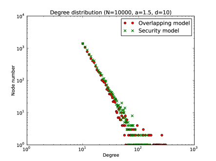
Figure 4: Power law of networks of the security model and the overlapping model

Let $G$ be a network constructed from the overlapping model. We define a community to be the induced subgraph of a homochromatic set. Clearly a community is connected. In Figure 5, we compare the distribution of conductances of a network of the security model and a network of the overlapping model with the same parameters as above.

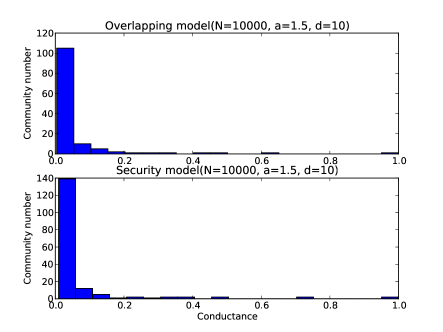
Figure 5: Distributions of conductances of communities for networks of both the security model and the overlapping model

From Figure 5, we know that distributions of conductances of all the communities are similar to each other, and almost all are small. This shows that networks constructed from the overlapping model are rich in small communities too.

The only difference between $G$ and networks constructed from the security model is that for each seed node of $G$, $v$ say, $v$ contains in $2$ communities. Our intuition is that overlapping communities undermine security of the networks.

In Figure 6, we compare the security of networks constructed from both the security model and the overlapping model for $n=10,000$, $a=1.5$, $d=10$, and $d_{1}=d_{2}=5$.

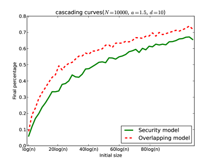
Figure 6: Security curves

Experiments in Figure 6 show that the network constructed from the security model is more secure than that of the overlapping model for attacks of all small-scales. This verifies that overlapping communities do undermine security of networks.

By this reason, we give up the phenomenon of overlapping communities in our elementary security theory of networks.

However it is still an open issue to fully understand the undermining of overlapping communities in security of networks. Solving this problem may provide a new way to enhance security of networks by distinguishing the different roles of a node in different communities. It is not surprising we may need a way to deal with the undermining effect of overlapping communities on security of networks. In general, it is an interesting open question to fully understand the roles of overlapping communities, since it seems universal in many real networks. Sometimes, overlapping communities are bad, for instance, every corrupt official confuses his/her public and private roles.

10 Conclusions and future directions

In this paper, we proposed definitions of security and robustness of networks to highlight the ability of complex networks to resist global cascading failures caused by a small number of deliberate attacks and random errors, respectively. We use the threshold cascading failure models to simulate information spreading in networks.

We introduced a security model of networks such that networks constructed from the model are provably secure under both uniform and random threshold cascading failure models, and simultaneously follow a power law, and satisfy the small world phenomenon with a remarkable $O(\log n)$ time algorithm to find a short path between arbitrarily given two nodes. This shows that networks constructed from the security model are secure, follow the natural property of power law, and allow a navigation of time complex $O(\log n)$.

The security model shows that dynamic and scale-free networks can be secure for which homophyly, randomness and preferential attachment are the underlying mechanisms, providing a principle for investigating the security of networks theoretically and generally.

Our security theorems explore some new discoveries between the roles of structures and of thresholds in the security of networks. The proofs of the security theorems provide a general framework to analyze both theoretically and practically security of networks.

It seems surprising that networks of the security model satisfy simultaneously all the properties stated in the three theorems, i.e., Theorems 3.1, 3.2 and 3.3, and that a merging of the principles in Theorems 3.1, 3.2 and 3.3 gives rise to the proofs of the security theorems, Theorems 4.1 and 4.2. This is a mathematical creation and mathematical beauty with immediate and far-reaching implications in network communication and network science.

On the other hand, the mechanisms of homophyly, randomness and preferential attachment of the security model are natural selections in evolutions of complex systems in both nature and society. This may explain the reason why networks of the security model have the remarkable properties here. This may also imply that the security model reflects some of the natural laws and social principles. This poses some fundamental questions such as: Does nature compute hard problems? Does nature evolve safely? Does society organize securely and stably? A possible approach to answering these questions could be to explore the physical, biological and social science understandings of the security model.

As usual, many real networks may not evolve as our security model. This is not surprised. There are always some differences between networks constructed from models and real networks. For instance, i) nontrivial networks of the PA model fail to have a community structure, but almost all real networks have, ii) nontrivial networks of the ER model fail to have a community structure or power law distribution, but almost all real networks have, and iii) networks of the small world model fail to have a power law, but almost all real networks have.

However, in our case, if real networks evolve in a way far from our security model, then it may imply that the real networks are highly unlikely to be secure, or worse, not even to be robust against a few random errors. This situation means that we do really and urgently need a theory to guarantee security of the networks in which we are living.

The mechanisms of the security model are natural selections in organizations of networks in both nature and society. However, the construction of networks in Definition 3.1 is carefully organized. A reader may wonder whether or not there is a cheaper construction of the networks with less ingredients than that in our definition. This could be possible, however, by our understanding, security of networks cannot be achieved freely, either in theory or in engineering.

A reader may wonder Definition 3.1 is a simple modification of the PA model, the two models should give similar networks. Why are the networks so different? It is true. However, there are two more new ideas introduced in the security model: the first is that every node has its own characteristic at the very beginning of its birth, that is, either remarkable (with new color) or normal (with old color), and the second is that two more natural mechanisms are introduced to remarkable nodes and normal nodes respectively. More importantly, the new ideas and the new mechanisms introduce ordering and combinatoric principles in the construction of networks. This perhaps explains that combinatorics plays a remarkable role in networks, and that purely probabilistic and single mechanism fails to capture complexity in nature and society.

By Theorem 4.1, for $\phi=O(\frac{1}{\log^{b}n})\ll 1/d$, networks generated from the security model is $\phi$-robust and $\phi$-secure. For the same constant $d$, the networks generated from both the PA model and the security model have the same average degree. By Theorem 4.1, the security threshold for the security model can be arbitrarily small as $n$ increases, while by Theorems 4.4 and 4.6, the robustness threshold for the PA model can only be the constant $1/d$. These theorems indicate that the structure of a network is key to the robustness and security although power law and small world properties exist in both models. Neither of these two properties is an obstacle to network robustness and security, while the small community phenomenon and connection patterns among communities play an essential role. Consequently, the security model provides an algorithm to construct dynamically networks which are secure against any attacks of small sizes under both uniform and random threshold cascading failure models, and which satisfy all the useful properties of usual networks.

Our results start a theoretical approach to network security. However there is a huge number of important issues open, for which we list some of them:

1. The role of homophyly exponent

   We notice that the homophyly exponent $a$ in Theorems 3.1,  4.1 and  4.2 is greater than $1,4$ and $6$ respectively, showing some differences among the fundamental theorem, the uniform threshold security theorem and the random threshold security theorem. The assumptions of $a>4$ and $a>6$ are essentially used in the proofs of Theorems  4.1 and  4.2 respectively. By Theorem 3.2, it seems necessary for $a$ to be large to make sure that almost all communities are strong. However for large $a$, the sizes of communities are also large, so that attack on a single node in a community may infect all nodes of the large community. Of course, for theoretical results, we only need to prove the theorems for all sufficiently large $n$, in which case, large $a$ is not a problem. In practice, the sizes of networks are limited, in which case, it is necessary to choose appropriate $a$ to make a balance to achieve the best possible security. Fortunately we have shown experimentally in  (?) that even for just $a>1$, for small $n$, networks of the security model are much more secure than that of both the ER and PA models under both random and uniform threshold cascading failure models. This poses a question to theoretically study the security theorems for just $a>1$, which will be more helpful for practical applications. Answering this question is not going to be easy, which calls for new analysis or new ideas.

   In our proofs, the average number of edges $d$ is assumed to be a constant. This assumption has no effect on theoretical results for all sufficiently large $n$. However, for fixed number $n$, the value $d$ plays a role. Usually the larger is $d$, the less secure is the network. This is reasonable, because, the larger is $d$, the denser is the network. However this problem is interested in only practice.

   In practice, many real networks may not be secure for which there are too many reasons. However, security may have only one reason. Our principles and theorems here provide a chance for us to examine the reasons why a given real network is insecure. Once we know the reasons of insecurity of a network, we may have ways to secure the network.

2. Security vs robustness

   Our theorems show that the security model in Definition 3.1 is secure, and that the preferential attachment model in  (?) is non-robust. It would be interesting to find a model of networks (dynamic, and with power law and small diameter property etc) that it is robust, but insecure. The significance of answering this question is to fully understand the robustness and the security of networks.

3. Criterions for security

   Our security model provides a principle for security. However, it is open to define criterions for security of a given network. This poses fundamental open questions such as: What are the theoretical criterions to measure quantitatively the security of real networks? What are the best possible algorithms to compute security indices of real networks?

4. Enhancing security

   A new fundamental question closely related to security applications is to enhance security of networks. In practice, we are given a network, $G$ say, and asked to make a minimal modification of $G$ to generate a network, $H$ say, such that $H$ keeps all the useful properties of $G$ and such that $H$ is much more secure than $G$. Our security model suggests some strategies for enhancing the security of networks. However, theoretical study of this issue is completely open.

5. Influence of structures

   To consider the influence of a structure, $G_{S}$ say (the induced subgraph of $S$), instead of just the set $S$ of nodes.

6. Fully understand the roles of mechanisms, structures in the security of networks

7. Security and game

   To introduce games in security strategies of networks.

8. Security and diffusion models

   To consider a variety of diffusion models according to different applications, for example, the independent cascading failure model in the context of marketing  (?),  (?).

9. Security of weighted networks

   To study the security of weighted and directed versions of networks to better capture new phenomena in the globalizing economic networks etc.

10. Robustness of networks

    Our results in Theorems  4.4 and  4.6 have implications in applications due to the fact that most real networks heavily depend on the preferential attachment scheme without guaranteeing the large threshold for all the vertices. This would imply that most real networks may not be even robust against random errors (or random attacks). And more importantly, the gap between the robustness threshold and non-robustness threshold is small, it could be very easy for a network to be non-robust. This means that robustness of networks is not an issue we can take for granted, and that global failure of real networks could be simply caused by random errors, instead of deliberate attacks. For this reason, robustness needs to be studied separately.

Finally we emphasize that our theory is to investigate the roles of structures, and the tradeoff between the role of structures and the role of thresholds in the security of networks. In engineering, security could be achieved by lifting the thresholds for all nodes, without considering the roles of structures of networks. A relatively long term challenge is to build a bridge between theory and engineering of security of networks. In practice, one more tough issue could be to distinguish positive and negative contents in the cascading procedure, which is already not purely a scientific problem.

References and Notes

- 1. R. Albert, H. Jeong, and A. L. Barabási. Error and attack tolerance of complex networks. Nature, 406:378–381, 2000.
- 2. R. M. Andersen and R. M. May. Infectious diseases of humans: dynamics and control. Oxford University Press, 1991. (book).
- 3. A. L. Barabási and R. Albert. Emergence of scaling in random networks. Science, 286:509–512, 1999.
- 4. L. Blume, D. Easley, J. Kleinberg, R. Kleinberg, and E. Tados. Which networks are least susceptible to cascading failures? Proceedings of 52nd Annual Symposium on Foundations of Computer Science, pages 393–402, 2011.
- 5. B. Bollobás and O. Riordan. The diameter of a scale-free random graph. Combinatorica, 24(1):5 C34, 2004.
- 6. H. Chernoff. A note on an inequality involving the normal distribution. The Annals of Probability, 9:533–535, 1981.
- 7. F. Chung and L. Lu. Complex graphs and networks. American Mathematical Society, 2006. (book).
- 8. P. Erdös and A. Rényi. On random graphs, i. Publ. Math., 6:290–297, 1959.
- 9. P. Erdös and A. Rényi. On the evolution of random graphsrandom graphs, i. Magyar Tud. Akad. Mat. Kutató Int. Kózl., 5:17–61, 1960.
- 10. J. Goldenberg, B. Libai, and E. Muller. Talk of the network: A complex systems look at the underlying process of the word-of-mouth. Marketing Letters, 12(3):211–223, 2001.
- 11. J. Goldenberg, B. Libai, and E. Muller. Using complex systems analysis to advanced marketing theory development. Academy of Marketing Science Review, 2001.
- 12. M. Granovetter. Threshold models of collective behavior. The American Journal of Sociology, 83(6):1420–1443, May 1978.
- 13. D. Kempe, J. Kleinberg, and E. Tardos. Maximizing the spread of influence through a social network. SIGKDD, 406:137–146, 2003.
- 14. A. Li, J. Li, Y. Pan, and P. Peng. Community structure is robust and universal in real networks. To appear, 2013.
- 15. A. Li, W. Zhang, Y. Pan, and X. Li. Security model of networks. To appear, 2013.
- 16. A. Li, W. Zhang, Y. Pan, and X. Li. Strategies for security of networks. To appear, 2013.
- 17. H. Mahmoud and R. Smythe. A survey of recursive trees. Theory of Probability and Mathematical Statistics, 51:1–27, 1995.
- 18. M. Mihail, C. H. Papadimitriou, and A. Saberi. On certain connectivity properties of the internet topology. Proc. 44th Annual Symposium on Foundations of Computer Science, pages 28–35, 2003.
- 19. S. Morris. Contagion. Review of Economic Studies, 67(2):57–78, 2000.
- 20. M. E. J. Newman. The structure and function of complex networks. SIAM Review, 45(2):167–256, 2003.
- 21. B. Pittel. Note on the heights of random recursive trees and random -ary search trees. Random Structures and Algorithms, 5:337–347, 1994.
- 22. F. Schweitzer, G. Fagiolo, D. Sornette, F. Vega-Redondo, A. Vespignani, and D. R. White. Economic networks: The new challenges. Science, 325(24), July 2009.
- 23. D. J. Watts. A simple model of global cascades on random networks. Proc. National Academy of Sciences, 99(9):5766–5771, 2002.
- 24. D. J. Watts and S. H. Strogatz. Collective dynamics of small world networks? Nature, 393:440–442, 1998.