Hosotani mechanism on the lattice

Abstract:

We explore the phase structure and symmetry breaking in four-dimensional SU(3) gauge theory with one spatial compact dimension on the lattice in the presence of fermions in the adjoint and fundamental representations with general boundary conditions. The eigenvalue phases of Polyakov loops and the associated susceptibility are measured on $16^{3}\times 4$ lattice. We establish a correspondence between the phases found on the lattice and the gauge symmetry breaking by the Hosotani mechanism.

capbtabboxtable[][]

1 Introduction

Symmetry breaking mechanisms play a central part in the unification of gauge forces. The gauge symmetry of a unified theory must be partially and spontaneously broken at low energies to describe the nature. In the standard model (SM) of electroweak interactions, the Higgs scalar field induces the symmetry breaking.

Among the several mechanism for gauge symmetry breaking there is the intriguing scenario of dynamical breaking by adding compact extra dimensions. In brief, when the extra dimensional space is not simply-connected, the non-vanishing phases $\theta_{H}$ of the Wilson line integral of gauge fields along a non-contractible loop in these extra dimensions can break the symmetry of the vacuum at one loop level [1, 2, 3, 4]. These phases $\theta_{H}$ are the Aharonov-Bohm (AB) phases in the extra dimensional space, which, despite its vanishing field strengths, affect physics leading to gauge symmetry breaking. This is the so called the Hosotani mechanism where the 4D Higgs boson is a part of gauge fields in higher dimensions. The values of $\theta_{H}$ are determined dynamically. Recently, the Hosotani mechanism has been applied to the electroweak interactions [5, 6, 7, 8, 9, 10, 11].

It should be pointed out that the Hosotani mechanism as a mechanism of gauge symmetry breaking has been so far established only in perturbation theory. It is based on the evaluation of the effective potential $V_{\rm eff}(\theta_{H})$ at the one-loop level. It is still not clear whether the mechanism operates at the non-perturbative level. This work is a first investigation on the non-perturbative realization of the Hosotani mechanism using lattice calculations. We take advantage of the fact that the Hosotani mechanism works in any dimensions such as $R^{n}\times S^{1}$, so we focus on the four-dimensional case ($R^{3}\times S^{1}$) in which the lattice gauge theory has been firmly established.

In this work, we would like to point out the connection between the phases identified by Cossu and D’Elia  [12] (in a work inspired by the semi-classical study [13]) and the Hosotani mechanism [14]. We also refine the connection by generalizing the boundary conditions for fermions in the fundamental representation. The rest of the report is presenting the theoretical background in Sect. 2 and the lattice calculations in Sect. 3. This proceeding is a summarized version of the full paper recently published online [15].

2 Continuum gauge theory on $R^{d-1}\times S^{1}$

As the simplest realization of the Hosotani mechanism, we consider SU(3) gauge theory coupled with fermions in the fundamental representation ($\psi_{\rm fd}$) and/or in the adjoint representation ($\psi_{\rm ad}$) in $d$-dimensional flat space-time with one spatial dimension compactified on $S^{1}$ [16, 17]. The circle $S^{1}$ has coordinate $y$ with a radius $R$ so that $y\sim y+2\pi R$. In terms of these quantities the Lagrangian density is given by:

$${\cal L}=-\frac{1}{2}{\rm Tr\,}F_{MN}F^{MN}+\bar{\psi}_{\rm fd}({\cal D}_{\rm fd}-m_{\rm fd})\psi_{\rm fd}+{\rm Tr\,}\bar{\psi}_{\rm ad}({\cal D}_{\rm ad}-m_{\rm ad})\psi_{\rm ad}$$ (1)

where ${\cal D}_{\rm fd}$ and ${\cal D}_{\rm ad}$ denote covariant Dirac operators. The gauge potentials $A_{M}=(A_{\mu},A_{y})$ ($\mu=1,\cdots,d-1$) and fermions $\psi_{\rm fd},\psi_{\rm ad}$ satisfy the following boundary conditions:

$$\begin{split}A_{M}(x,y+2\pi R)&=VA_{M}(x,y)V^{-1},\\ \psi_{\rm fd}(x,y+2\pi R)=e^{i\alpha_{\rm fd}}\,V\,\psi_{\rm fd}(x,y),\quad&\psi_{\rm ad}(x,y+2\pi R)=e^{i\alpha_{\rm ad}}\,V\,\psi_{\rm ad}(x,y)V^{-1},\end{split}$$ (2)

where $V\in SU(3)$. With these boundary conditions the Lagrangian density is single-valued on $S^{1}$, namely ${\cal L}(x,y+2\pi R)={\cal L}(x,y)$, so that physics is well-defined on the manifold $R^{d-1}\times S^{1}$. It has been proven (see [4]) that physics is independent of $V$ at the quantum level so we adopt $V=I$ hereafter.

There is a residual gauge invariance given the boundary conditions (2). Under a gauge transformation $\Omega$, the boundary condition (2) with $V=I$ is maintained, provided $\Omega(x,y+2\pi R)=\Omega(x,y)$. The eigenvalues of $W=P\exp\left(ig\int_{0}^{2\pi R}dy\,A_{y}(x,y)\right)$ are gauge invariant. They are denoted as $\big{\{}e^{i\theta_{1}},e^{i\theta_{2}},e^{i\theta_{3}}\big{\}}$ where $\sum_{j=1}^{3}\theta_{j}=0~{}(\bmod~{}2\pi)~{}$. Constant configurations of $A_{y}\not=0$ with $A_{\mu}=0$ yield vanishing field strengths $\langle F_{MN}\rangle=0$, but in general give $W\neq I$, or nontrivial $\theta_{H}$. We stress that this class of configurations is not gauge equivalent to $A_{M}=0$ if we want to keep the boundary conditions constant. The $\theta_{j}$’s are the elements of AB phase $\theta_{H}$ in the extra dimension. These are the dynamical degrees of freedom of the gauge fields affecting physical quantities as in the Aharonov-Bohm effect in quantum mechanics.

2.1 Symmetry breaking

To see the effect of the AB phases on the spectrum of gauge bosons we expand the fields of the SU(3) gauge theory on $R^{d-1}\times S^{1}$ in Kaluza-Klein modes of the extra-dimension: [4] where each KK mode has the following mass-squared in the $(d-1)$-dimensional space-time.

$$\begin{split}A_{\mu}^{(n)}:&\left(m_{A}^{(n)}\right)_{jk}^{2}=\frac{1}{R^{2}}\Big{(}n+\frac{\theta_{j}-\theta_{k}}{2\pi}\Big{)}^{2}~{},\\ \psi_{\rm fd}^{(n)}:\left(m_{\rm fd}^{(n)}\right)_{j}^{2}=\frac{1}{R^{2}}\Big{(}n+\frac{\theta_{j}+\alpha_{\rm fd}}{2\pi}\Big{)}^{2}+&m_{\rm fd}^{2}~{},\psi_{\rm ad}^{(n)}:\left(m_{\rm ad}^{(n)}\right)_{jk}^{2}=\frac{1}{R^{2}}\Big{(}n+\frac{\theta_{j}-\theta_{k}+\alpha_{\rm ad}}{2\pi}\Big{)}^{2}+m_{\rm ad}^{2}~{}.\end{split}$$

In particular, from the gauge boson mass of the zero-mode $(m_{A}^{(0)})^{2}$, we can discuss the remaining gauge symmetry realization after the compactification. Because the mass is given by the difference $\theta_{j}-\theta_{k}$, it is classically expected that the mass spectrum becomes SU(3) asymmetric unless $\theta_{1}=\theta_{2}=\theta_{3}\ ({\rm mod}\ 2\pi)$. However, as a dynamical degree of freedom, $\theta_{H}$ has quantum fluctuation. In the confined phase, these fluctuations are large enough for the SU(3) symmetry to remain intact. For a moderate gauge coupling and sufficiently small $R$, $\theta_{H}$ would take nontrivial values to break SU(3) symmetry depending on the fermion content. To determine which value of $\theta_{H}$ is realized at the quantum level, it is convenient to evaluate the effective potential $V_{\rm eff}(\theta_{H})$, whose global minimum is given by the vacuum expectation values (VEVs) of $\theta_{H}$. We show the plots for the two flavors of adjoint fermions case in figure 1 in order to compare with the lattice simulations.

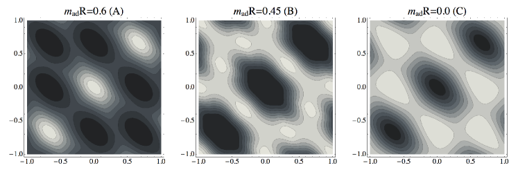
Figure 1: Effective potential for the case of $N_{\rm ad}=2$ adjoint fermion with periodic boundary condition ($\alpha_{\rm ad}=0$) for the values of $m_{\rm ad}R$ in $d=4$. They are corresponding to the $X$ phase, the $B$ phase and the $C$ phase, respectively. Lower values of $V_{{\rm eff}}$ are indicated by lighter colors.

In lattice simulations one measures the VEVs of $P_{3}$ and $P_{8}$. The absolute value of $P_{3}$ is strongly affected by quantum fluctuations of $\theta_{H}$ and is reduced at strong gauge couplings. The phase of $P_{3}$, on the other hand, is less affected by quantum fluctuations in the weak coupling regime so that transitions from one phase to another should be seen as changes in the phase of $P_{3}$. Indeed, this is precisely what has been found in ref. [12]. The classifications of the phases are summarized in Table 1, where we also include the confined phase, denoted by $X$, in which $\theta_{H}$ fluctuate and take all possible values.

Table 1: Classification of the location of the global minima of $V_{\rm eff}(\theta_{H})$. In the last column the names of the corresponding phases termed in ref. [12] are also listed for $X,A,B$ and $C$.

	$\theta_{H}=(\theta_{1},\theta_{2},\theta_{3})$ with permutations	$P_{3}$	$P_{8}$	Global Symmetry, Phase
$X$	Large quantum fluctuations	$0$	$-\frac{1}{8}$	SU(3), confined
$A_{1};A_{2,3}$	(0,0,0); $(\pm\hbox{$\frac{2}{3}$}\pi,\pm\hbox{$\frac{2}{3}$}\pi,\pm\hbox{$\frac{2}{3}$}\pi)$	1; $e^{\pm 2\pi i/3}$	1	SU(3), deconfined
$B_{1}$;$B_{2,3}$	$(0,\pi,\pi)$; $(\pm\hbox{$\frac{2}{3}$}\pi,\mp\hbox{$\frac{1}{3}$}\pi,\mp\hbox{$\frac{1}{3}$}\pi)$	$-\hbox{$\frac{1}{3}$}$; $\hbox{$\frac{1}{3}$}e^{\mp\pi i/3}$	0	SU(2) $\times$ U(1), split
$C$	$(0,\hbox{$\frac{2}{3}$}\pi,-\hbox{$\frac{2}{3}$}\pi)$	0	$-\frac{1}{8}$	U(1) $\times$ U(1), reconfined

3 Lattice results

We compute Polyakov loops $P_{3}$ and $P_{8}$ on the $16^{3}\times 4$ volume gauge configurations sampled with the weight $e^{-S_{g}-S_{f}}$. The transition points were determined using the susceptibility $\chi_{\Omega}=N_{x}^{3}\left(\langle\Omega^{2}\rangle-\langle\Omega\rangle^{2}\right)$ of the observable $\Omega\in\{|P_{3}|,P_{8}\}$ which scales with the lattice volume at the phase transitions. In connection to the perturbative results, where the relevant parameter is $m_{\rm fd}R$ or $m_{\rm ad}R$, increasing $\beta$ has the effect of decreasing those parameters, due to the running of the renormalized fermion mass in the lattice unit. We estimate statistical errors by employing the jackknife method with appropriate bin sizes to incorporate any auto-correlations.

3.1 Phase structure with adjoint fermions

In the numerical simulation for $(N_{\rm ad},N_{\rm fd})=(2,0)$, we use bare masses $m_{\rm ad}a=ma=0.05$ and $0.10$ changing $\beta$ covering the range $5.3\leq\beta\leq 6.5$. Periodic boundary condition is used ($\alpha_{\rm ad}=0$) in the compact direction, which is different from the case with anti-periodic boundary conditions (finite temperature) where only the confined and deconfined phases are realized [18]. The essentially same setup is included in the study of ref. [12]. To explore the phase structure in heavier mass region, we also examine bare masses $m_{\rm ad}a=ma=0.50$ and $0.80$ for the range of $5.5\leq\beta\leq 9.8$ and $5.5\leq\beta\leq 20.0$, respectively.

We summarize the phase space and the phase transition points obtained in figure 2. For further discussion on the properties of these transitions, a more detailed study on the finite size scaling has to be done.

Because the $B$-$C$ transitions are hard to observe clearly from the Polyakov loops or the susceptibilities, we estimate empirically the interval where the transition occurs by inspection of the $\theta$s distributions. Due to the subjective character of the analysis, we do not quote any error, just an interval where the transition is occurring.

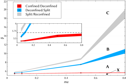
Figure 2: Phase diagram for the $N_{\rm ad}=2$ adjoint fermion system with periodic boundary condition in the compact dimension. In the window, the $X$-$A$ transition line is compared with the pure gauge case (dashed line) [19].

3.2 Phase structure with fundamental fermions

We study the dependence of $P_{3}$ and $P_{8}$ on the boundary phase $\alpha_{\rm fd}$ for several values of $\beta$ in the presence of fundamental fermions with U(1) phase $\alpha_{\rm fd}$ as the boundary condition. This setup is formally equivalent to finite temperature QCD with an imaginary chemical potential $\nu=\pi+\alpha_{\rm fd}$. To test the perturbative predictions we carry out a numerical simulation with $(N_{\rm ad},N_{\rm fd})=(0,4)$. Since we are interested in the symmetries of the Polyakov loop, we determine the locations of the transition points by the peak points of $\chi_{|P_{3}|}$, contrary to the previous works where the chiral condensate was used to locate the critical points. The resulting distributions of $P_{3}$ are shown in Fig. 3.

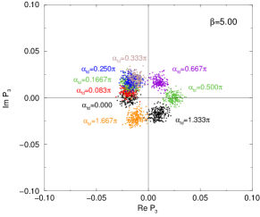
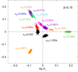
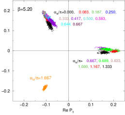
Figure 3: (First three panels) Distributions of $P_{3}$ obtained on gauge ensembles with a variation of $\alpha_{\rm fd}$ for $\beta=5.00$ (left), $5.15$ (center) and $5.20$ (right). The degrees of $\alpha_{\rm fd}$ used in the calculation are indicated with the corresponding data. Overall, data points with same degrees of $\alpha_{\rm fd}$ are indicated by same colors.

Having confirmed the Roberge-Weiss periodic structure [20] and using the symmetry about $\alpha_{\rm fd}=\pi/3$, we concentrate on the region $0\leq\alpha_{\rm fd}<\pi/3$ to determine the $A$-$B$ (or, confined-deconfined) transition points. For $\alpha_{\rm fd}=n\pi/12$ with $n=0,1,2,3,4$, we investigate the susceptibilities of $|P_{3}|$ and $P_{8}$ along with the analysis in the previous section. We obtain the well known Roberge-Weiss phase diagram in terms of the phases predicted by the Hosotani mechanism. The deconfined phases at high $\beta$ are identified as the $A_{i}$ phases of table 1.

3.3 Eigenvalues of the Wilson line

In the previous sections we identified four phases in the case of adjoint fermions with periodic boundary condition. The comparison of the measured values for $P_{3}$ and $P_{8}$ with the ones listed in Table 1 suggests that these phases are related to the Hosotani mechanism. In order to clarify the connection of these phases with the perturbative effective potential predictions we show the results of the eigenvalues of the Wilson line wrapping around the compact dimension.

In this analysis care must be taken in order to disentangle the effect of the Haar measure for SU(3) [21] $\prod_{i>j}\sin^{2}\frac{\theta_{i}-\theta_{j}}{2}$. This measure term gives a strong repulsive force for the eigenvalues. We estimated numerically the effect of this term and renormalized the lattice results accordingly. The $A$, $B$ and $C$ phases should show different degeneracy of eigenvalues as shown in table 1.

The results of our investigations are shown in the panels of Fig. 4. Each one of them displays the density plots for the Polyakov loop eigenvalue phases $(\theta_{1},\theta_{2})$. Smearing is applied to the configuration before measurements to filter the ultraviolet modes that are not relevant for the location of the minima of $V_{\rm eff}$.

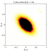
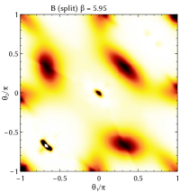
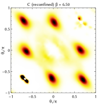
Figure 4: Density plots at several $\beta$’s for the Polyakov Loop eigenvalues (in the $\theta_{1}/\pi$ - $\theta_{2}/\pi$ plane). Here the original data is divided by the Haar measure distribution. From left to right, the panels correspond to the $X$, $A$, $B$ and $C$ phases. The first panel is white as a result of the calculation. Darker colors denote the highest density regions.

Although a bit noisy because of the procedure, it shows the expected features of the perturbative potential, and can be directly compared with the perturbative prediction of Fig. 1. The plots, from left to right, are respectively the $X$, $A$, $B$, and $C$ phases. The distribution in the $X$ (confined) phase is a constant i.e. unity so the plot is a white image, which is a manifestation of a uniform random distribution of the eigenvalues in the two dimensional plane. An interesting finding is that the $C$ phase shows a completely different behavior from the confined one. The eigenvalues are now not distributed in a random fashion but located in peaks around the $Z_{3}$ symmetric values $\theta_{i}=0,\pm 2\pi/3$ (again some artifacts appear), with maximal repulsion between them (see a semi-classical analysis e.g. in [22]). All the four predicted phases are clearly represented by the data, which is a strong indication of the realization of the Hosotani mechanism in 3+1 dimensions even at the non-perturbative level.

Numerical simulations are performed on the Hitachi SR16K at Kyoto University and the SR16K and the IBM System Blue Gene Solution at KEK under its Large-Scale Simulation Program (No. T12-09 and 12/13-23). This work was supported in part by grants from the Ministry of Education and Science (No. 20244028, 23104009, 21244036). G. C and J. N are supported in part by Strategic Programs for Innovative Research (SPIRE) Field 5. H. H is partly supported by NRF Research Grant 2012R1A2A1A01006053 (HH) of the Republic of Korea.

References

- [1] Hosotani Y. Phys.Lett., B126:309, 1983.
- [2] Davies A. and McLachlan A. Phys.Lett., B200:305, 1988.
- [3] Davies A. and McLachlan A. Nucl.Phys., B317:237, 1989.
- [4] Hosotani Y. Annals Phys., 190:233, 1989.
- [5] Burdman G. and Nomura Y. Nucl.Phys., B656:3–22, 2003.
- [6] Csaki C., Grojean C., and Murayama H. Phys.Rev., D67:085012, 2003.
- [7] Agashe K., Contino R., and Pomarol A. Nucl.Phys., B719:165–187, 2005.
- [8] Cacciapaglia G., Csaki C., and Park S.C. JHEP, 0603:099, 2006.
- [9] Medina A.D., Shah N.R., and Wagner C.E. Phys.Rev., D76:095010, 2007.
- [10] Hosotani Y., Oda K., Ohnuma T., and Sakamura Y. Phys.Rev., D78:096002, 2008.
- [11] Hosotani Y., Noda S., and Uekusa N. Prog.Theor.Phys., 123:757–790, 2010.
- [12] Cossu G. and D’Elia M. JHEP, 0907:048, 2009.
- [13] Unsal M. and Yaffe L.G. Phys.Rev., D78:065035, 2008.
- [14] Hosotani Y. AIP Conf.Proc., 1467:208–213, 2012.
- [15] Cossu G., Hatanaka H., Hosotani Y., and Noaki J.I. arXiv:1309.4198 [hep-lat].
- [16] Hatanaka H. Prog.Theor.Phys., 102:407–418, 1999.
- [17] Hosotani Y. Proceedings of SCGT2004, pages 17–34, 2005.
- [18] Karsch F. and Lutgemeier M. Nucl.Phys., B550:449–464, 1999.
- [19] Fukugita M., Okawa M., and Ukawa A. Phys.Rev.Lett., 63:1768, 1989.
- [20] Roberge A. and Weiss N. Nucl.Phys., B275:734, 1986.
- [21] Bruckmann F. arXiv:1007.4052 [hep-ph], 2010.
- [22] Poppitz E., Schäfer T., and Ünsal M. JHEP, 1303:087, 2013.