A Bayesian framework for functional
time series analysis

Abstract

The paper introduces a general framework for statistical analysis of functional time series from a Bayesian perspective. The proposed approach, based on an extension of the popular dynamic linear model to Banach-space valued observations and states, is very flexible but also easy to implement in many cases. For many kinds of data, such as continuous functions, we show how the general theory of stochastic processes provides a convenient tool to specify priors and transition probabilities of the model. Finally, we show how standard Markov chain Monte Carlo methods for posterior simulation can be employed under consistent discretizations of the data.

Keywords: Functional time series, dynamic linear model, probability on Banach spaces.

1 Introduction

Time series data consisting of individual high or infinite dimensional observations are becoming more and more common in many applied areas. As a consequence there is a need to develop models and algorithms for the analysis and forecasting of this kind of data. Clearly any statistically sound model should account for the temporal dependence of the data, in addition to a possibly complex correlation structure within the observations made at a specific time point. Statistician have been working on methods for the analysis of functional data for several years; early references are Ramsay and Dalzell (1991) and Grenander (1981), the books by Ramsay and Silverman (2006, 2002), Ramsay et al. (2009), and Ferraty and Vieu (2006) provide good entry points to the recent literature. More recently, there has been an interest also in models and tools for time series of functional data, see for example Aue et al. (2009); Ding et al. (2009); Horváth et al. (2010); Hyndman and Shang (2009); Kargin and Onatski (2008); Shen (2009). The review papers by Mas and Pumo (2010) and Hörmann and Kokoszka (2012) contain up-to-date references, while the books by Bosq (2000) and Horváth and Kokoszka (2012) provide a comprehensive background. However, a fatisfactory treatment of functional time series from a Bayesian perspective has been so far elusive. Our research aims at filling this gap, providing a flexible and easy-to-use class of models for Bayesian analysis of functional time series.

From a methodological point of view, the main focus of the paper is the extension of the highly successful dynamic linear model to function spaces. Related references are Falb (1967) and Bensoussan (2003). Their extensions, however, are different from the one suggested in the present paper, since they focus on continuous-time processes and, most importantly, they do not provide algorithms that are well-suited for practical applications.

The layout of the paper is as follows. We introduce in Section 2 the basic notions related to Banach space-valued random variables that will be needed for the subsequent development. The model we propose is discussed in Section 3, where also Kalman filter and smother in the infinite dimensional setting are discussed. Section 4 focus on a practical example in which the model is applied to a time series of continuous functions. Concluding remarks are contained in Section 5.

2 Functional random variables

In this section we briefly introduce Banach space-valued random variables and the extension of the notions of expectation and covariance to this type of random variables. We also discuss Gaussian distributions on Banach spaces. Most of the material of this section is covered in great detail in the monographs by Bogachev (1998) and Da Prato and Zabczyk (1992). We consider in the following only separable Banach spaces. While this is a strong requirement from a theoretical perspective, it is not a serious limitation for applications, since almost all Banach spaces of functions used in practice are separable, the most notable exception being probably $L^{\infty}$, the space of essentially bounded (equivalence classes of) functions on a given measurable space. The symbol , possibly with a subscript, will be used to denote a separable, but otherwise general, Banach space. We will use the notation $\mathord{\mathcal{L}}(\B,{}_{1})$ for the Banach space consisting of all continuos linear operators mapping to ₁. In the case when ${}_{1}=\B$ we will abbreviate the notation to $\mathord{\mathcal{L}}(\B)$. ^∗ will denote the Banach space of all continuous linear functionals on , i.e., ${}^{*}=\mathord{\mathcal{L}}(\B,\R)$. Recall that, for any $A\in\mathord{\mathcal{L}}(\B,{}_{1})$, the adjoint operator $A^{*}\in\mathord{\mathcal{L}}({}_{1}^{*},{}^{*})$ is defined, for every $b_{1}^{*}\in{}_{1}^{*}$, to be the element of ^∗ defined as $b\mapsto b_{1}^{*}(A(b))$.

A Banach space-valued random variable $X$ is a measurable function $X$ defined on a given probability space and taking values in

$$X:(\Omega,\mathord{\mathcal{F}})\rightarrow(\B,\mathord{\mathcal{B}}),$$

where $\mathord{\mathcal{B}}$ denotes Borel $\sigma$-algebra of subsets of . The separability assumption implies that $\mathord{\mathcal{B}}$ is also the $\sigma$-algebra generated by the continuous linear functionals on , i.e., the smallest $\sigma$-algebra with respect to which all elements of ^∗ are measurable.

If $X$ is a -valued random variable and $\mathord{\mathrm{E}}(\|X\|)<\infty$, then for every $f\in{}^{*}$ the real-valued random variable $f(X)$ has finite expectation, since $\mathord{\mathrm{E}}(|f(X)|)\leq\|f\|\mathord{\mathrm{E}}(\|X\|)<\infty$. Clearly the functional $f\mapsto\mathord{\mathrm{E}}(f(X))$ is linear in $f\in{}^{*}$ and the previous inequality shows that it is continuous at zero, hence defining a continuous linear functional on ^∗, i.e., an element of ^∗∗. It can be shown that this element of ^∗∗ has the form $f\mapsto f(\mu)$ for a vector $\mu\in\B$. We call this vector the expected value, or expectation, of $X$ and write $\mu=\mathord{\mathrm{E}}(X)$. The expected value can be characterized as the unique element of such that $\mathord{\mathrm{E}}(f(X))=f(\mu)$ $\forall f\in{}^{*}$. Expected values commute with continuous linear operators in the following sense: if $A\in\mathord{\mathcal{L}}(\B,{}_{1})$ and $X$ is a -valued random variable with expected value $\mu$, then the $B_{1}$-valued random variable $X_{1}=A(X)$ has expected value given by $\mathord{\mathrm{E}}(X_{1})=A(\mu)$.

An argument along similar lines can be used to show that if $\mathord{\mathrm{E}}(\|X\|^{2})<\infty$, then the mapping $\lambda:{}^{*}\times{}^{*}\longrightarrow\R$ specified by

$$\lambda(f,g)=\mathord{\mathrm{E}}\bigl{(}f(X-\mu)g(X-\mu)\bigr{)},\qquad f,g\in{}^{*}$$

defines a bilinear function which, in turn, identifies a unique continuous linear operator $\Lambda\in\mathord{\mathcal{L}}({}^{*},\B)$ via the identity $\lambda(f,g)=f(\Lambda(g))$. The operator $\Lambda$ is called the covariance operator, or just covariance, of $X$, while the bilinear function $\lambda$ is called the covariance function of $X$. Covariance operator and covariance function are two equivalent ways of providing the same information about the distribution of $X$. A covariance operator is symmetric and positive, i.e., $g(\Lambda(f))=f(\Lambda(g))$ and $f(\Lambda(f))\geq 0$ for all $f,g\in{}^{*}$. Unlike what happens in ⁿ, where every symmetric, positive definite matrix is a covariance matrix, not all symmetric and positive elements of $\mathord{\mathcal{L}}({}^{*},\B)$ are valid covariance operators. In fact, $\Lambda\in\mathord{\mathcal{L}}({}^{*},\B)$ is a covariance operator if and only if there is a sequence $\{x_{n}\}$ in with $\sum_{n}\|x_{n}\|^{2}<\infty$ such that $\Lambda(f)=\sum_{n}f(x_{n})x_{n}$ for all $f\in{}^{*}$.

If $X_{1}$ and $X_{2}$ are $B_{1}$- and $B_{2}$-valued random variables, respectively, with $\mathord{\mathrm{E}}(\|X_{i}\|^{2})<\infty$, $i=1,2$, and expected values $\mu_{1}$ and $\mu_{2}$, then we can define the covariance function between $X_{1}$ and $X_{2}$ to be the bilinear operator $\lambda_{12}:{}_{1}^{*}\times{}_{2}^{*}\longrightarrow\R$ defined by

$$\lambda_{12}(f_{1},f_{2})=\mathord{\mathrm{E}}\bigl{(}f_{1}(X_{1}-\mu_{1})f_{2}(X_{2}-\mu_{2})\bigr{)},\qquad f_{i}\in{}_{i}^{*},i=1,2.$$

The corresponding covariance operator $\Lambda_{1,2}\in\mathord{\mathcal{L}}({}_{2}^{*},{}_{1})$ between $X_{1}$ and $X_{2}$ is determined by the relationship

$$f_{1}(\Lambda_{12}(f_{2}))=\lambda_{12}(f_{1},f_{2}),\qquad f_{i}\in{}_{i}^{*},i=1,2.$$

A -valued random variable $X$ with expected value $\mu$ and covariance $\Lambda$ has a Gaussian distribution if for every $f\in{}^{*}$ the real-valued random variable $f(X)$ has a Gaussian distribution. In this case, we write $X\sim\mathord{\mathcal{N}}(\mu,\Lambda)$. It is not hard to show that $X$ has a Gaussian distribution if and only if its characteristic functional (Fourier transform) has the form

$$\psi(f)=\mathord{\mathrm{E}}\big{(}e^{if(X)}\big{)}=\exp\left\{if(\mu)-\tfrac{1}{2}\lambda(f,f)\right\},\qquad f\in{}^{*},$$

where $\lambda$ is the covariance function associated with $\Lambda$. Using this characterization, it is easy to see that, if $A\in\mathord{\mathcal{L}}(\B,{}_{1})$, then $A(X)\sim\mathord{\mathcal{N}}_{{}_{1}}(A(\mu),A\Lambda A^{*})$.

Unlike what happens in the finite-dimensional case, for a general there are valid covariance operators that are not the covariance operator of any -valued Gaussian random variable.

To conclude this section, let us recall the definition of regular conditional distribution. Let $Z$ be a random variable taking values in a measurable space $(\bS,\mathcal{S})$, and let $\mathord{\mathcal{G}}$ be a sub-$\sigma$-algebra of $\mathord{\mathcal{F}}$. A function $\pi:\Omega\times\mathcal{S}:\longrightarrow\R$ is a regular conditional distribution (r.c.d.) for $Z$ given $\mathord{\mathcal{G}}$ if the following two conditions hold.

1. For every $\omega\in\Omega$, $\pi(\omega,\cdot)$ is a probability on $(\bS,\mathcal{S})$.

2. For every $S\in\mathcal{S}$, $\pi(\cdot,S)$ is a version of $\mathord{\mathrm{P}}(Z\in S\mid\mathord{\mathcal{G}})$.

A standard result about r.c.d.’s is that if is a Polish space with Borel $\sigma$-algebra $\mathcal{S}$, then a r.c.d. for $Z$ given $\mathord{\mathcal{G}}$ exists. In particular, this is the case when is a separable Banach space endowed with its Borel $\sigma$-algebra. For notational simplicity, in the following sections we will typically omit the explicit dependence on $\omega$ of a regular conditional probability.

3 Functional dynamic linear model

We define in this section the functional dynamic linear model (FDLM) and we discuss the extension of Kalman filtering and smoothing recursions, valid in the finite-dimensional case, to the case of Banach space-valued states and observations. We assume that the reader is familiar with the basic elements of dynamic linear models (DLMs) from a Bayesian perspective in the standard case of finite-dimensional states and observations, as found for example in West and Harrison (1997) or Petris et al. (2009).

Let , the observation space, and , the state space, be separable Banach spaces endowed with their Borel $\sigma$-algebras. Consider infinite sequences $Y_{1},Y_{2},\dots$ and $X_{0},X_{1},\dots$ of - and -valued random variables. We say that they form a state space model if $\{X_{t}\}$ is a Markov chain and, for every $t$, the conditional distribution of $Y_{t}$ given all the other random variables depends on the value of $X_{t}$ only. Let $F\in\mathord{\mathcal{L}}(\Gban,\Fban)$ and $G\in\mathord{\mathcal{L}}(\Gban)$. An FDLM is a state space model satisfying the following distributional assumptions:

$$X_{0} \sim\mathord{\mathcal{N}}\big{(}m_{0},C_{0}\big{)},$$ (1)

$$X_{t}|X_{t-1}=x_{t-1} \sim\mathord{\mathcal{N}}\big{(}G(x_{t-1}),W\big{)},$$

$$Y_{t}|X_{t}=x_{t} \sim\mathord{\mathcal{N}}\big{(}F(x_{t}),V\big{)},$$

where $m_{0}\in\Gban$, $C_{0}$ and $W$ are covariance operators on , and $V$ is a covariance operator on . The definition as well as Kalman recursions, given below, can be extended in an obvious way to time-dependent operators $F$, $G$, $V$ and $W$; we use the time-invariant version of the model in this paper mainly for notational simplicity. As for the finite dimensional DLM, quantities of immediate interest related to this model are the filtering and smoothing distributions, that is, the conditional distribution of the state $X_{t}$ given the observations $Y_{1:t}$ (filtering distribution) and the conditional distribution of $X_{s}$, for $s\leq t$, given $Y_{1:t}$ (smoothing distribution). In the finite dimensional DLM all the conditional distributions of a set of states or future observations, given past observations, are Gaussian. This property extends to the FDLM. One practical issue that arises in the infinite dimensional model is that observations, while conceptually infinite dimensional, have to be discretized at some point, in order to allow proper data storage and processing. Clearly this discretization leads in general to a loss of information. However, in this context, one would hope that the inference based on the discretized data is almost as good as the inference based on the complete, functional data, at least if the discretized version of the data is still rich enough to carry most of the information from the complete data. In other words, one needs to show a continuity property of the inference – the filtering and smoothing distributions – with respect to the discretization. If the discretization is defined in a way that is consistent with the infinite dimensional process, then one can show that for the FDLM the continuity property mentioned above holds.

In order not to clutter the notation, we discuss the continuity of the posterior distribution with respect to a sequence of discretizations only in the case of one functional observation $Y$ and one functional state $X$. Clearly, the argument extends to the FDLM setting in a straightforward way. Let $D_{n}\in\mathord{\mathcal{L}}(\Fban,{}^{d_{n}})$, $n\geq 1$, be a sequence of linear, continuous operators. The $D_{n}$’s define by composition a sequence of random variables $Y_{n}=D_{n}(Y)$, where $Y_{n}$ is ${}^{d_{n}}$-valued. We require that $\sigma(Y_{n})\uparrow\sigma(Y)$, which formally expresses the fact that the information carried by the discretized version $Y_{n}$ approximates better and better the information carried by the complete datum $Y$, coinciding with it in the limit. Let $\pi_{n}$ be a r.c.d of $X$ given $Y_{n}$ and $\pi$ a r.c.d. of $X$ given $Y$. Then

$$\lim_{n\rightarrow\infty}\pi_{n}=\pi\qquad\text{almost surely},$$

where the limit is in the topology of weak convergence of probability measures. Moreover, since all the $\pi_{n}$ are Gaussian distributions, and the class of Gaussian distributions is closed under the topology of weak convergence, one can also deduce that $\pi$ is a Gaussian distribution as well.

An example of a sequence of discretizations of the type described above is the following. Consider $\Fban=C([0,1])$. For $n\geq 1$ and $1\leq k\leq 2^{n}$, let $q_{n,k}=k\,2^{-n}$ and define $D_{n}:C([0,1])\longrightarrow{}^{2^{n}}$ by the formula

$$D_{n}(y)=\big{(}y(q_{n,1}),\dots,y(q_{n,2^{n}})\big{)}.$$

Note that the same sequence of discretizing operators, evaluating a function at the points of a sequence of finer and finer grids in [0,1], would not be well defined if the functional datum $Y$ were an element of $L^{2}([0,1])$, as it is often assumed in the FDA literature. In fact, in that case the value of the function at any given point is not even well defined, since elements of $L^{2}([0,1])$ are equivalence classes of functions, defined up to equality almost everywhere.

Kalman filter and smoother, as well as the simulation smoother, or forward filtering backward sampling algorithm (FFBS), which draws a sample from the smoothing distribution, can be extended to the FDLM. The following theorem provides the Kalman filter recursion for the FDLM.

Theorem 1.

Consider the FDLM (1) and, for $n\geq 1$, let $D_{n}\in\mathord{\mathcal{L}}(\Fban,{}^{d_{n}})$. Define $Y_{t,n}=D_{n}(Y_{t})$. Assume that $\sigma(Y_{t,n})\uparrow\sigma(Y_{t})$ and suppose that

$$X_{t-1}\mid Y_{1:t-1}\sim\mathord{\mathcal{N}}(m_{t-1},C_{t-1}).$$

Then the updating of the filtering distribution proceeds as follows.

1. One-step-ahead forecast distribution for the state:

   $$X_{t}\mid Y_{1:t-1}\sim\mathord{\mathcal{N}}(a_{t},R_{t}),$$

   with $a_{t}=G(m_{t-1})$ and $R_{t}=GC_{t-1}G^{*}+W$.

2. One-step-ahead forecast distribution for the observation:

   $$Y_{t}\mid Y_{1:t-1}\sim\mathord{\mathcal{N}}(f_{t},Q_{t}),$$

   with $f_{t}=F(a_{t})$ and $Q_{t}=FR_{t}F^{*}+V$.

3. One-step-ahead forecast distribution for the discretized observation:

   $$Y_{t,n}\mid Y_{1:t-1}\sim\mathord{\mathcal{N}}(f_{t,n},Q_{t,n}),$$

   with $f_{t,n}=D_{n}(f_{t})$ and $Q_{t,n}=D_{n}Q_{t}D_{n}^{*}$.

4. Filtering distribution at time $t$, given the discretized observation:

   $$X_{t}\mid Y_{1:-1},Y_{t,n}\sim\mathord{\mathcal{N}}(m_{t,n},C_{t,n}),$$

   with $m_{t,n}=a_{t}+R_{t}F^{*}D_{n}^{*}Q_{t,n}^{-1}(Y_{t,n}-f_{t,n})$ and $C_{t,n}=R_{t}-R_{t}F^{*}D_{n}^{*}Q_{t,n}^{-1}D_{n}FR_{t}$.

5. Filtering distribution at time $t$:

   $$\pi_{t}=\lim_{n\rightarrow\infty}\pi_{t,n}\qquad\text{a.s.},$$

   where $\pi_{t,n}$ is a r.c.d. for $X_{t}$ given $(Y_{1:t-1},Y_{t,n})$ and $\pi_{t}$ is a r.c.d. for $X_{t}$ given $Y_{1:t}$. Moreover, $\pi_{t}$ is a.s. a Gaussian distribution.

Proof of Theorem 1.

We will first derive the joint conditional distribution of $(X_{t},Y_{t})$ given $Y_{1:t-1}$, from which the conditional distributions in 1 and 2 will easily follow. The dual of $\Gban\times\Fban$ can be identified with ${}^{*}\times{}^{*}$ noting that the element $(x^{*},y^{*})\in{}^{*}\times{}^{*}$ can be associated to the element of $(\Gban\times\Fban)^{*}$ defined by

$$\widetilde{(x^{*},y^{*})}:(x,y)\mapsto x^{*}(x)+y^{*}(y).$$

Moreover, every element in $(\Gban\times\Fban)^{*}$ has that form for a unique choice of $x^{*}$ and $y^{*}$. We will make use of the following matrix notation for operators. If $A\in\mathord{\mathcal{L}}(\A,{}_{1})$, $B\in\mathord{\mathcal{L}}(\B,{}_{1})$, $C\in\mathord{\mathcal{L}}(\A,{}_{1})$, and $D\in\mathord{\mathcal{L}}(\B,{}_{1})$, the matrix

$$\begin{bmatrix}A&B\\ C&D\end{bmatrix}$$

denotes the element of $\mathord{\mathcal{L}}(\A\times\B,{}_{1}\times{}_{1})$ defined by

$$\A\times\B\ni(a,b)\mapsto\big{(}A(a)+B(b),C(a)+D(b)\big{)}.$$

It is easy to show that any element of $\mathord{\mathcal{L}}(\A\times\B,{}_{1}\times{}_{1})$ can be uniquely represented in the matrix form written above. Let us compute the conditional characteristic functional of $(X_{t},Y_{t})$ given $Y_{1:t-1}$. For $x^{*}\in{}^{*}$ and $y^{*}\in{}^{*}$ we have

$$\psi(x^{*},y^{*}) =\mathord{\mathrm{E}}\Big{(}\exp\bigg{\{}i\big{(}x^{*}(X_{t})+y^{*}(Y_{t})\big{)}\bigg{\}}|Y_{1:t-1}\Big{)}$$

$$=\mathord{\mathrm{E}}\Big{(}\mathord{\mathrm{E}}\Big{(}\exp\bigg{\{}i\big{(}x^{*}(X_{t})+y^{*}(Y_{t})\big{)}\bigg{\}}|X_{t},Y_{1:t-1}\Big{)}|Y_{1:t-1}\Big{)}$$

$$=\mathord{\mathrm{E}}\Big{(}\exp\bigg{\{}ix^{*}(X_{t})+iy^{*}(F(X_{t}))-\frac{1}{2}y^{*}(V(y^{*}))\bigg{\}}|Y_{1:t-1}\Big{)}$$

$$=\mathord{\mathrm{E}}\Big{(}\exp\bigg{\{}i\big{(}x^{*}+F^{*}y^{*}\big{)}(X_{t})\bigg{\}}|Y_{1:t-1}\Big{)}\exp\bigg{\{}-\frac{1}{2}y^{*}(V(y^{*}))\bigg{\}}$$

$$=\mathord{\mathrm{E}}\Big{(}\mathord{\mathrm{E}}\Big{(}\exp\bigg{\{}i\big{(}x^{*}+F^{*}y^{*}\big{)}(X_{t})\bigg{\}}|X_{t-1},Y_{1:t-1}\Big{)}|Y_{1:t-1}\Big{)}\exp\bigg{\{}-\frac{1}{2}y^{*}(V(y^{*}))\bigg{\}}$$

$$=\mathord{\mathrm{E}}\Big{(}\exp\bigg{\{}i\big{(}x^{*}+F^{*}y^{*}\big{)}(G(X_{t-1}))\bigg{\}}|Y_{1:t-1}\Big{)}$$

$$\qquad\exp\bigg{\{}-\frac{1}{2}\Big{[}(x^{*}+F^{*}y^{*})\big{(}W(x^{*}+F^{*}y^{*})\big{)}+y^{*}(V(y^{*}))\Big{]}\bigg{\}}$$

$$=\exp\bigg{\{}i\big{(}x^{*}+F^{*}y^{*}\big{)}(G(m_{t-1}))$$

$$\qquad-\frac{1}{2}\Big{[}(x^{*}G+F^{*}y^{*}G)\big{(}C_{t-1}(x^{*}G+F^{*}y^{*}G)\big{)}$$

$$\qquad+(x^{*}+F^{*}y^{*})\big{(}W(x^{*}+F^{*}y^{*})\big{)}+y^{*}(V(y^{*}))\Big{]}\bigg{\}}$$

$$=\exp\bigg{\{}i\big{[}x^{*}(G(m_{t-1}))+y^{*}(FG(m_{t-1}))\big{]}$$

$$\qquad-\frac{1}{2}\Big{[}x^{*}\big{(}(GC_{t-1}G^{*}+W)(x^{*})\big{)}$$

$$\qquad+x^{*}\big{(}(GC_{t-1}G^{*}F^{*}+WF^{*})(y^{*})\big{)}+y^{*}\big{(}(FGC_{t-1}G^{*}+FW)(x^{*})\big{)}$$

$$\qquad+y^{*}\big{(}(FGC_{t-1}G^{*}F^{*}+FWF^{*}+V)(y^{*})\big{)}\Big{]}\bigg{\}}$$

This shows that the conditional distribution of $(X_{t},Y_{t})$ given $Y_{1:t-1}$ is Gaussian with mean $(a_{t},f_{t})$ and covariance operator

$$\begin{bmatrix}R_{t}&R_{t}F^{*}\\ FR_{t}&Q_{t}\end{bmatrix},$$

from which parts 1 and 2 of the theorem follow. Part 3 is an immediate consequence of part 2, when one considers how Gaussian distributions transform under the application of a continuous linear operator. As far as part 4 is concerned, if $X_{t}$ were a finite dimensional random variable, then the result would be a straightforward application of the well-known theorem on Normal correlation (Lipster and Shiryayev; 1972; Barra; 1981). It is simple to verify that the proof of that result carries over to the case where $X_{t}$ is a Banach space-valued random variable, as long as the conditioning random variable is finite dimensional. Finally, part 5 of the theorem follows from the result on discretization of observations discussed above. ∎

As far as the smoothing distribution is concerned, since under our modelling assumptions the joint distribution of $(X_{0:t},Y_{1:t})$ is Gaussian, all its marginal distributions, including that of $(X_{s},Y_{1:t})$ are Gaussian as well. It follows that the conditional distribution of $X_{s}$ given $Y_{1:t}$ is again Gaussian; that is, the smoothing distribution of $X_{s}$ is Gaussian, as in the finite dimensional setting. In general, however, the smoothing means and covariances do not have a simple explicit form. For the purpose of applications this is not a big impediment, since the analysis is always performed on a discretized version of the data, to which the usual smoothing recurrence applies (Petris et al.; 2009). The inference obtained from the discretized version of the FDLM converges, as the discretization gets finer, to the inference that one would obtain from the complete functional data, by the argument discussed before Theorem 1.

4 Application to $C([0,1])$-valued time series

In order to define a Gaussian -valued random variable one can rely, when is a Banach space of functions, on the theory of stochastic processes. When $\B=C([0,1])$, a stochastic process with continous sample paths can be interpreted as a -valued random variable. Let us spell out the equivalence, which will be used in the rest of the present section. Suppose $\zeta=\{\zeta_{t}:t\in[0,1]\}$ is a stochastic process with continous trajectories. Note that every $\zeta_{t}$ is a random variable, i.e., $\zeta_{t}=\zeta_{t}(\omega)$. Then, since the sample paths are continuous, one can define the function $\tilde{\zeta}:\Omega\longrightarrow C([0,1])$ by setting

$$\tilde{\zeta}(\omega):t\mapsto\zeta_{t}(\omega),\qquad\text{$t\in[0,1]$ and $\omega\in\Omega$.}$$ (2)

The following theorem shows that $\tilde{\zeta}$ is a $C([0,1])$-valued random variable and specifies its mean and covariance function. In addition, it shows that $\tilde{\zeta}$ has a Gaussian distribution if the process $\zeta$ does. Recall that, by Riesz representation theorem, $C([0,1])^{*}$ can be identified with the Banach space of all signed measures on the Borel sets of [0,1], denoted below by $\mathcal{M}([0,1])$. For $\eta\in\mathcal{M}([0,1])$ and $x\in C([0,1])$ we will use the notation

$$\eta(x):=\int_{[0,1]}x(t)\eta(dt).$$

Theorem 2.

For the function defined in (2), the following hold.

1. $\tilde{\zeta}$ is a measurable function from $(\Omega,\mathord{\mathcal{F}})$ to the Banach space $C([0,1])$ endowed wih its Borel $\sigma$-algebra.

2. If, in addition, the process $\zeta$ possesses second moments, then the expected value and the covariance function of $\tilde{\zeta}$ are given by

   $$C([0,1])\ni\mathord{\mathrm{E}}(\tilde{\zeta}):t\mapsto\mathord{\mathrm{E}}(\zeta_{t}),$$

   $$\lambda(\eta,\tau)=\int_{[0,1]^{2}}\gamma(u,v)\eta(du)\tau(dv),\qquad\eta,\tau\in\mathcal{M}([0,1]),$$

   where $\gamma(u,v)=\mathord{\mathrm{Cov}}(\zeta_{u},\zeta_{v})$. The covariance operator of $\tilde{\zeta}$ is

   $$\Lambda(\eta)=\int_{[0,1]}\gamma(u,\cdot)\,\eta(du),\qquad\eta\in\mathcal{M}([0,1]).$$ (3)

3. If, in addition, the process $\zeta$ is Gaussian, then $\tilde{\zeta}$ has a Gaussian distribution.

Proof.

1. See Bosq (2000), Example 1.10.

2. Let $\eta,\tau\in\mathcal{M}([0,1])$. In view of Jordan decomposition $\eta=\eta^{+}-\eta^{-}$, so we can assume, without real loss of generality, that $\eta$ and $\tau$ are positive measures. By a straightforward application of Fubini’s theorem, we have

   $$\mathord{\mathrm{E}}\bigg{(}\int_{[0,1]}\tilde{\zeta}(t)\eta(dt)\bigg{)} =\int_{\Omega}\int_{[0,1]}\zeta_{t}(\omega)\eta(dt)P(d\omega)$$

   $$=\int_{[0,1]}\int_{\Omega}\zeta_{t}(\omega)P(d\omega)\eta(dt)$$

   $$=\int_{[0,1]}\mathord{\mathrm{E}}(\zeta_{t})\eta(dt)=\eta\big{(}\mathord{\mathrm{E}}(\zeta_{\cdot})\big{)}.$$

   Let $m=\mathord{\mathrm{E}}(\tilde{\zeta})$. Then, using Fubini’s theorem,

   $$\lambda(\eta,\tau) =\mathord{\mathrm{E}}\big{(}\eta(\tilde{\zeta}-m)\tau(\tilde{\zeta}-m)\big{)}$$

   $$=\int_{\Omega}\Big{(}\int_{[01]}\big{(}\zeta_{u}(\omega)-m(u)\big{)}\eta(du)\Big{)}\Big{(}\int_{[0,1]}\big{(}\zeta_{v}(\omega)-m(v)\big{)}\tau(dv)\Big{)}\mathord{\mathrm{P}}(d\omega)$$

   $$=\int_{\Omega}\Big{(}\int_{[01]^{2}}\big{(}\zeta_{u}(\omega)-m(u)\big{)}\big{(}\zeta_{v}(\omega)-m(v)\big{)}\eta(du)\tau(dv)\Big{)}\mathord{\mathrm{P}}(d\omega)$$

   $$=\int_{[01]^{2}}\Big{(}\int_{\Omega}\big{(}\zeta_{u}(\omega)-m(u)\big{)}\big{(}\zeta_{v}(\omega)-m(v)\big{)}\mathord{\mathrm{P}}(d\omega)\Big{)}\eta(du)\tau(dv)$$

   $$=\int_{[01]^{2}}\gamma(u,v)\eta(du)\tau(dv).$$

   The form of the covariance operator follows immediately from the expression giving the covariance function.

3. Let $\eta\in\mathcal{M}([0,1])$ and consider the discretization operator defined for any $x\in C([0,1])$ by

   $$x_{n}(t)=\mathord{\mathrm{I}}_{\{0\}}(t)x(0)+\sum_{j=1}^{n}\mathord{\mathrm{I}}_{\Delta_{n,j}}(t)x(j/n),$$

   where

   $$\Delta_{n,j}=\left(\frac{j-1}{n},\frac{j}{n}\right].$$

   It is clear that the map $x\mapsto x_{n}$ is non-expansive, i.e., $\|y_{n}-x_{n}\|\leq\|y-x\|$, and therefore continuous. It follows that by applying this operator to $\tilde{\zeta}$ we obtain another $C([0,1])$-valued random variable, say $\tilde{\zeta}_{n}$. For any fixed $\omega\in\Omega$,

   $$\eta\big{(}\tilde{\zeta}(\omega)\big{)}=\eta(\{0\})\zeta_{0}(\omega)+\sum_{j=1}^{n}\eta(\Delta_{n,j})\zeta_{j/n}(\omega).$$

   Since the stochastic process $\zeta$ is Gaussian, the joint distribution of $(\zeta_{0},\zeta_{1/n},\ldots,\zeta_{1})$ is Gaussian, hence $\eta(\tilde{\zeta})$ is Gaussian as well. It is also easy to show that, with probability one, $\tilde{\zeta}_{n}\rightarrow\tilde{\zeta}$ as $n\rightarrow\infty$. Since $\eta$, as a functional on $C([0,1])$, is continuous, it follows that $\eta(\tilde{\zeta}_{n})\rightarrow\eta(\tilde{\zeta})$ almost surely and, a fortiori, $\eta(\tilde{\zeta}_{n})\stackrel{{\scriptstyle d}}{{\rightarrow}}\eta(\tilde{\zeta})$. Since the class of Gaussian distributions on is closed with respect to the topology of weak convergence, we conclude that $\eta(\tilde{\zeta})$ has a Gaussian distribution.

∎

In our numerical example below we will make extensive use of Theorem 2, using it to define Gaussian $C([0,1])$-valued random variables starting from the Ornstein-Uhlenbeck process, having mean zero and covariance function

$$\gamma(u,v)=\frac{\sigma^{2}}{2\beta}\exp\bigl{\{}-\beta|u-v|\bigr{\}},$$ (4)

where $\sigma^{2}$ and $\beta$ are positive parameters. These random variables will be used, in turn, as building blocks to set up an FDLM.

We consider a data set consisting in hourly measurements on the log scale of electricity demand, over the previous hour, collected at a distribution station in the Northeastern region of the United States from January 2006 to December 2010. We consider the data to be a discretized version of a daily functional time series. Since it is reasonable to assume that electricity demand follows a continuous path over time, we will model the data as $C([0,1])$-valued random variables. Figure 1 shows the full data set.

Figure 1: Electricity demand

For scalar time series, a specific DLM that has been successfully used to model observations with a constant or slowly changing mean is the so-called local level model. This simply consists in a random walk for a univariate state, which is observed with noise. The model can be immediately extended to functional data, setting $\Fban=\Gban$, $F=G=\mathord{\boldsymbol{1}}$ in (1), where, for any Banach space , $\mathord{\boldsymbol{1}}$ denotes the identity operator on . We take $m_{0}$ to be the zero element of $C([0,1])$, and the covariance operators $C_{0}$, $W$ and $V$ to be of the form (3), with $\gamma(u,v)$ specified in (4). The parameters $\sigma^{2}$ and $\beta$ in  (4) are different for the three covariance operators and, while we fix their value when we define $C_{0}$, so as to obtain a prior distribution for the initial state that is only vaguely informative, we estimate the parameters of $V$ and $W$, $(\sigma^{2}_{V},\beta_{V})$ and $(\sigma^{2}_{W},\beta_{W})$, respectively. The inference was carried out using MCMC, simulating in turn the latent states via the forward filtering backward sampling (FFBS) algorithm (Carter and Kohn; 1994; Früwirth-Schnatter; 1994; Shephard; 1994), and the parameters $\sigma^{2}_{V},\beta_{V},\sigma^{2}_{W},\beta_{W}$. We coded the sampler in the statistical programming language R (R Core Team; 2013), using also the contributed packages zoo (Zeileis and Grothendieck; 2005) for data manipulation and graphing, and dlm (Petris; 2010), which contains an implementation of FFBS.

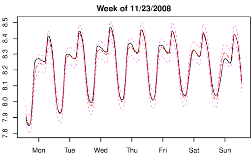
Figure 2: One week of electricity demand (solid line), with smoothed demand (two dash) and 90% probability bands (dashed)

The prior used for the two variance parameters is an inverse gamma, which is conditionally conjugate for this particular model, when the latent states are included in the simulation, while the two remaining parameters $\beta_{V}$ and $\beta_{W}$ were updated with a random walk Metropolis-Hastings step on the log scale. Figure 2 displays, for one particular week, the observations together with the smoothed states for those seven days, and 90% probability bands, obtained from the MCMC output. The fit is good, showing that the functional model, despite the small number of parameters, is flexible enough to adapt and learn the general daily pattern of electricity demand on any given day.

$\sigma^{2}_{V}$	$\log\beta_{V}$	$\sigma^{2}_{W}$	$\log\beta_{W}$
$2.76\cdot 10^{-04}$	$-2.83$	$2.14\cdot 10^{-04}$	$-3.23$
$9.86\cdot 10^{-08}$	$2.30\cdot 10^{-03}$	$1.33\cdot 10^{-07}$	$2.51\cdot 10^{-03}$
$(2.70,2.81)\cdot 10^{-4}$	$(-2.89,-2.76)$	$(2.09,2.20)\cdot 10^{-4}$	$(-3.30,-3.16)$

Table 1: Posterior estimates, with Monte Carlo standard errors and 90% posterior probability intervals

In terms of the inference on the model parameters, Table 1 summarizes posterior estimates of the four parameters, together with MC standards errors and 90% posterior probability intervals. MC standard errors are computed using Sokal’s estimator (Sokal; 1989), as implemented in the R package dlm.

5 Conclusions

The model presented in the paper is an important step forward in the methodology of analysis of functional time series. For such kind of data it provides a much more flexible setting compared to functional ARMA models (Bosq; 2000; Horváth and Kokoszka; 2012). The FDLM allows to extend to the functional setting most of the standard structural time series models (Harvey; 1989) that have proved extremely useful for the analysis and forecasting of finite dimensional time series. Among the advantages of the FDLM proposed in the paper, we note that the specification of a particular model is in most cases relatively straightforward, as illustrated in Section 4, and the practical implementation of the posterior sampling can be done using standard MCMC algorithms.

References

- (1)
- Aue et al. (2009) Aue, A., Gabrys, R., Horváth, L. and Kokoszka, P. (2009). Estimation of a change-point in the mean function of functional data, Journal of Multivariate Analysis 100: 2254–2269.
- Barra (1981) Barra, J. (1981). Mathematical Basis of Statistics, Academic Press.
- Bensoussan (2003) Bensoussan, A. (2003). Some remarks on linear filtering theory for infinite dimensional system, in A. Rantzer and C. Byrnes (eds), Directions in Mathematical System Theory and Optimization, Springer-Verlag.
- Bogachev (1998) Bogachev, V. (1998). Gaussian measures, American Mathematical Society.
- Bosq (2000) Bosq, D. (2000). Linear processes in function spaces, Springer-Verlag, New York.
- Carter and Kohn (1994) Carter, C. and Kohn, R. (1994). On Gibbs sampling for state space models, Biometrika 81: 541–553.
- Da Prato and Zabczyk (1992) Da Prato, G. and Zabczyk, J. (1992). Stochastic equations in infinite dimensions, Cambridge University Press.
- Ding et al. (2009) Ding, G., Lin, L. and Zhong, S. (2009). Functional time series prediction using process neural networks, Chinese Physics Letters 26.
- Falb (1967) Falb, P. (1967). Infinite-dimensional filtering: the Kalman-Bucy filter in Hilbert space, Information and Control 11: 102–137.
- Ferraty and Vieu (2006) Ferraty, F. and Vieu, P. (2006). Nonparametric Functional Data Analysis, Springer-Verlag.
- Früwirth-Schnatter (1994) Früwirth-Schnatter, S. (1994). Data augmentation and dynamic linear models, Journal of Time Series Analysis 15: 183–202.
- Grenander (1981) Grenander, U. (1981). Abstract Inference, Wiley.
- Harvey (1989) Harvey, A. (1989). Forecasting, Structural Time Series Models and the Kalman filter, Cambridge University Press, Cambridge.
- Hörmann and Kokoszka (2012) Hörmann, S. and Kokoszka, P. (2012). Functional time series, in T. Subba Rao, S. Subba Rao and C. Rao (eds), Handbook of Statistics, Vol. 30, Elsevier.
- Horváth et al. (2010) Horváth, L., Hušková, M. and Kokoszka, P. (2010). Testing the stability of the functional autoregressive process, Journal of Multivariate Analysis 101: 352–367.
- Horváth and Kokoszka (2012) Horváth, L. and Kokoszka, P. (2012). Inference for Functional Data with Applications, Springer.
- Hyndman and Shang (2009) Hyndman, R. and Shang, H. (2009). Forecasting functional time series, Journal of the Korean Statistical Society 38: 199–211.
- Kargin and Onatski (2008) Kargin, V. and Onatski, A. (2008). Curve forecasting by functional autoregression, Journal of Multivariate Analysis 99: 2508–2526.
- Lipster and Shiryayev (1972) Lipster, R. and Shiryayev, A. (1972). Statistics of conditionally Gaussian random sequences, Proceedings of the Sixth Berkeley Symposium on Mathematical Statistics and Probability, Univ. California Press, Berkeley.
- Mas and Pumo (2010) Mas, A. and Pumo, B. (2010). Linear processes for functional data, in F. Ferraty and Y. Romain (eds), The Oxford handbook of functional data, Oxford University Press.
-
Petris (2010)
Petris, G. (2010).
An R package for dynamic linear models, Journal of Statistical
Software 36(12): 1–16.
http://www.jstatsoft.org/v36/i12/ - Petris et al. (2009) Petris, G., Petrone, S. and Campagnoli, P. (2009). Dynamic linear models with R, Springer-Verlag, New York.
-
R Core Team (2013)
R Core Team (2013).
R: A Language and Environment for Statistical Computing, R
Foundation for Statistical Computing, Vienna, Austria.
ISBN 3-900051-07-0.
http://www.R-project.org/ - Ramsay and Dalzell (1991) Ramsay, J. and Dalzell, C. (1991). Some tools for functional data analysis, Journal of the Royal Statistical Society, Series B 53: 539–572.
- Ramsay et al. (2009) Ramsay, J., Hooker, G. and Graves, S. (2009). Functional Data Analysis with R and Matlab, Springer-Verlag, New York.
- Ramsay and Silverman (2002) Ramsay, J. and Silverman, B. (2002). Applied functional data analysis, Springer-Verlag, New York.
- Ramsay and Silverman (2006) Ramsay, J. and Silverman, B. (2006). Functional Data Analysis, 2nd edn, Springer-Verlag, New York.
- Shen (2009) Shen, H. (2009). On modeling and forecasting time series of smooth curves, Technometrics 51: 227–238.
- Shephard (1994) Shephard, N. (1994). Partial non-Gaussian state space models, Biometrika 81: 115–131.
- Sokal (1989) Sokal, A. (1989). Monte Carlo Methods in Statistical Mechanics: Foundations and New Algorithms, Cours de Troisiéme Cycle de la Physique en Suisse Romande, Lausanne.
- West and Harrison (1997) West, M. and Harrison, J. (1997). Bayesian Forecasting and Dynamic Models, 2nd edn, Springer-Verlag, New York.
-
Zeileis and Grothendieck (2005)
Zeileis, A. and Grothendieck, G. (2005).
zoo: S3 infrastructure for regular and irregular time series, Journal of Statistical Software 14(6): 1–27.
http://www.jstatsoft.org/v14/i06/