Nearly Optimal Sample Size in Hypothesis Testing for High-Dimensional Regression

Abstract

We consider the problem of fitting the parameters of a high-dimensional linear regression model. In the regime where the number of parameters $p$ is comparable to or exceeds the sample size $n$, a successful approach uses an $\ell_{1}$-penalized least squares estimator, known as Lasso.

Unfortunately, unlike for linear estimators (e.g., ordinary least squares), no well-established method exists to compute confidence intervals or p-values on the basis of the Lasso estimator. Very recently, a line of work [JM13b, JM13a, vdGBR13] has addressed this problem by constructing a debiased version of the Lasso estimator. In this paper, we study this approach for random design model, under the assumption that a good estimator exists for the precision matrix of the design. Our analysis improves over the state of the art in that it establishes nearly optimal average testing power if the sample size $n$ asymptotically dominates $s_{0}(\log p)^{2}$, with $s_{0}$ being the sparsity level (number of non-zero coefficients). Earlier work obtains provable guarantees only for much larger sample size, namely it requires $n$ to asymptotically dominate $(s_{0}\log p)^{2}$.

In particular, for random designs with a sparse precision matrix we show that an estimator thereof having the required properties can be computed efficiently. Finally, we evaluate this approach on synthetic data and compare it with earlier proposals.

1 Introduction

In the random design model for linear regression, we are given $n$ i.i.d. pairs $(Y_{1},X_{1}),\dotsc,(Y_{n},X_{n})$ with $X_{i}\in{\mathbb{R}}^{p}$. The response variables $Y_{i}$ are given by

$$Y_{i}\,=\,\langle\theta_{0},X_{i}\rangle+W_{i}\,,\;\;\;\;\;\;\;\;W_{i}\sim{\sf N}(0,\sigma^{2})\,.$$ (1)

Here $\langle\,\cdot\,,\,\cdot\,\rangle$ is the standard scalar product in ${\mathbb{R}}^{p}$, and $\theta_{0}\in{\mathbb{R}}^{p}$ is an unknown but fixed vector of parameters. In matrix form, letting $Y=(Y_{1},\dotsc,Y_{n})^{\sf T}$ and denoting by ${\mathbf{X}}$ the design matrix with rows $X_{1}^{\sf T},\dotsc,X_{n}^{\sf T}$, we have

$$Y\,=\,{\mathbf{X}}\,\theta_{0}+W\,,\;\;\;\;\;\;\;\;W\sim{\sf N}(0,\sigma^{2}{\rm I}_{n\times n})\,.$$ (2)

The goal is to estimate the unknown vector of parameters $\theta_{0}\in{\mathbb{R}}^{p}$ from the observations $Y$ and ${\mathbf{X}}$. We are interested in the high-dimensional setting where the number of parameters is larger than the sample size, i.e., $p>n$, but the number of non-zero entries of $\theta_{0}$ is smaller than $p$. We denote by $S\equiv{\rm supp}(\theta_{0})\in[p]$ the support of $\theta_{0}$, i.e., the set of non-zero coefficients, and let $s_{0}\equiv|S|$ be the sparsity level.

In the last decade, there has been a burgeoning interest in parameter estimation in high-dimensional setting. A particularly successful approach is the Lasso [Tib96, CD95] estimator which promotes sparse reconstructions through an $\ell_{1}$ penalty:

$$\widehat{\theta}(Y,{\mathbf{X}};\lambda)\equiv\arg\min_{\theta\in{\mathbb{R}}^{p}}\Big{\{}\frac{1}{2n}\|Y-{\mathbf{X}}\theta\|^{2}_{2}+\lambda\|\theta\|_{1}\Big{\}}\,.$$ (3)

In case the right hand side has more than one minimizer, one of them can be selected arbitrarily for our purposes. We will often omit the arguments $Y$, ${\mathbf{X}}$, as they are clear from the context.

The Lasso is known to perform well in terms of prediction error $\|{\mathbf{X}}(\widehat{\theta}-\theta_{0})\|^{2}_{2}$ and estimation error, as measured for instance by $\|\widehat{\theta}-\theta_{0}\|_{2}^{2}$ [BvdG11]. In this paper we address the –far less understood– problem of assessing uncertainty and statistical significance, e.g., by computing confidence intervals or p-values. This problem is particularly challenging in high dimension since good estimators, such as the Lasso, are by necessity non-linear and hence do not have a tractable distribution.

More specifically, we are interested in testing null hypotheses of the form:

$$H_{0,i}:\,\theta_{0,i}=0\,,\quad\quad\text{ for }i\in[p]\,,$$ (4)

and assigning $p$-values for these tests. Rejecting $H_{0,i}$ corresponds to inferring that $\theta_{0,i}\neq 0$. A related question is the one of computing confidence intervals. Namely, for a given $i\in[p]$, and $\alpha\in(0,1)$ we want to determine $\underline{\theta}_{i},\overline{\theta}_{i}\in{\mathbb{R}}$ such that

$${\mathbb{P}}(\theta_{i}\in[\underline{\theta}_{i},\overline{\theta}_{i}])\geq 1-\alpha\,.$$ (5)

1.1 Main idea and summary of contributions

A series of recent papers have developed the idea of ‘de-biasing’ the Lasso estimator $\widehat{\theta}$, by defining

$$\widehat{\theta}^{u}=\widehat{\theta}+\frac{1}{n}\,M{\mathbf{X}}^{\sf T}(Y-{\mathbf{X}}\widehat{\theta})\,.$$ (6)

Here $M\in{\mathbb{R}}^{p\times p}$ is a matrix that depends on the design matrix ${\mathbf{X}}$, and aims at decorrelating the columns of ${\mathbf{X}}$. A possible interpretation of this construction is that the term ${\mathbf{X}}^{\sf T}(Y-{\mathbf{X}}\widehat{\theta})/(n\lambda)$ is a subgradient of the $\ell_{1}$ norm at the Lasso solution $\widehat{\theta}$. By adding a term proportional to this subgradient, we compensate for the bias introduced by the $\ell_{1}$ penalty. It is worth noting that $\widehat{\theta}^{u}$ is no longer a sparse estimator. In certain regimes, and for suitable choices of $M$, it was proved that $\widehat{\theta}^{u}-\theta_{0}$ is approximately Gaussian with mean $0$, hence leading to the construction of p-values and confidence intervals.

More specifically, let $\Sigma={\mathbb{E}}(X_{1}X_{1}^{\sf T})$ be the population covariance matrix, and $\Omega=\Sigma^{-1}$ denote the precision matrix. In [JM13b], the present authors assumed the precision matrix to be known and proposed to use $M=c\Omega$, for an explicit constant $c$. A plug-in estimator for $\Omega$ was also suggested for sparse covariances $\Sigma$. Furthermore, asymptotic validity and minimax optimality of the method were proven for uncorrelated Gaussian designs ($\Sigma={\rm I}$). A conjecture was derived for a broad class of covariances using statistical physics arguments. De Geer, Bühlmann and Ritov [vdGBR13] used a similar construction with $M$ an estimate of $\Omega$, which is appropriate for sparse precision matrices $\Omega$. These authors prove validity of their method for sample size $n$ that asymptotically dominates $(s_{0}\log p)^{2}$. In [JM13a], the present authors propose to construct $M$ by solving a convex program that aims at optimizing two objectives. First, control the bias of $\widehat{\theta}^{u}$, and second minimize the variance of $\widehat{\theta}^{u}_{i}$. Minimax optimality was established for sample size $n$ that asymptotically dominates $(s_{0}\log p)^{2}$, without however requiring $\Omega$ to be sparse. Additional related work can be found in [Büh12, ZZ11] .

Note that nearly optimal estimation via the Lasso is possible for significantly smaller sample size, namely for $n\geq Cs_{0}\log p$, for some constant $C$ [CT07, BRT09]. This suggests the following natural question

Is it possible to design a minimax optimal test for hypotheses $H_{0,i}$, for optimal sample size $n=O(s_{0}\log p)$?

While the results of [JM13b] suggest a positive answer, they assume $\Omega$ to be known, and apply only asymptotically as $n,p\to\infty$. In this paper we partially answer this question, by proving the following results.

General subgaussian designs.

We do not make any assumption on the rows of ${\mathbf{X}}$ except that they are independent and identically distributed, with common law $p_{X}$ with subgaussian tails, and non-singular covariance. This model is well suited for statistical applications wherein the pairs $(Y_{i},X_{i})$ are drawn at random from a population.

Our results in this case holds conditionally on the availability of an estimator $\widehat{\Omega}$ of the precision matrix such that $\|\widehat{\Omega}-\Omega\|_{\infty}=o(1/\sqrt{\log p})$. Then, a testing procedure is developed that is minimax optimal with nearly optimal sample size, namely for $n$ that asymptotically dominates $s_{0}(\log p)^{2}$. Here ‘optimality’ is measured in terms of the average power of tests for hypotheses $H_{0,i}$ with average taken over the coordinates $i\in[p]$. To be more specific, the testing procedure is constructed based on the debiased estimator $\widehat{\theta}^{u}$, where we set $M=\widehat{\Omega}$.

Subgaussian designs with sparse inverse covariance.

In this case, the rows are subgaussian with a common covariance $\Sigma$, such that $\Omega=\Sigma^{-1}$ is sparse. For this model, an estimator with the required properties exists, and was used in [vdGBR13]. We can therefore establish unconditional results and prove optimality of the present test.

With respect to earlier analysis [vdGBR13], our results apply to much smaller sample size, namely $n$ needs to dominate $s_{0}(\log p)^{2}$ instead of $(s_{0}\log p)^{2}$. On the other hand, guarantees are only provided with respect to average power of the test. Roughly speaking, our results in this case imply that the method of [vdGBR13] has significantly broader domain of validity than initially expected.

While the assumption of sparse inverse covariance is admittedly restrictive, it arises naturally in a number of contexts. For instance, it is relevant for the problem of learning sparse Gaussian graphical models [MB06]. In this case, the set of edges incident on a specific vertex can be encoded in the vector $\theta_{0}$. It also played a pivotal role in compressed sensing, as one of the first model in which an optimal tradeoff between sparsity $s_{0}$ and sample size $n$ was proven to hold [CT05, DT05, Wai09].

Covariance estimators satisfying the condition $\|\widehat{\Omega}-\Omega\|_{\infty}=o(1/\sqrt{\log p})$ can be constructed under other structural assumptions than sparsity. Our general theory allows to build hypothesis testing methods for each of these cases. We expect this to spur progress in other settings as well.

Finally, we evaluate our procedure on synthetic data, comparing its performance with the method of [JM13a].

1.2 Definitions and notations

Throughout $\Sigma={\mathbb{E}}\{X_{1}X_{1}^{{\sf T}}\}$ will be referred to as the covariance, and $\Omega\equiv\Sigma^{-1}\in{\mathbb{R}}^{p\times p}$ as the precision matrix. Without loss of generality, we will assume that the columns of ${\mathbf{X}}$ are normalized so that $\Sigma_{ii}=1$. (This normalization is only assumed for the analysis, and is not required for the hypothesis testing procedure or the construction of confidence intervals.)

For a matrix $A$ and set of indices $I,J$, we let $A_{I,J}$ denote the submatrix formed by the rows in $I$ and columns in $J$. Also, $A_{I,\cdot}$ (resp. $A_{\cdot,I}$) denotes the submatrix containing just the rows (resp. columns) in $I$. Likewise, for a vector $v$, $v_{I}$ is the restriction of $v$ to indices in $I$. The maximum and the minimum singular values of $A$ are respectively denoted by $\sigma_{\max}(A)$ and $\sigma_{\min}(A)$. We write $\|v\|_{p}$ for the standard $\ell_{p}$ norm of a vector $v$ (omitting the subscript in the case $p=2$) and $\|v\|_{0}$ for the number of nonzero entries of $v$. For a matrix $A$, $\|A\|_{p}$ is its $\ell_{p}$ operator norm, and $|A|_{p}$ is the elementwise $\ell_{p}$ norm, i.e., $|A|_{p}=(\sum_{i,j}|A_{ij}|^{p})^{1/p}$. Further $|A|_{\infty}=\max_{i,j}|A_{ij}|$. We use the notation $[n]$ for the set $\{1,\dotsc,n\}$. For a vector $v$, ${\rm supp}(v)$ represents the positions of nonzero entries of $v$.

The standard normal distribution function is denoted by $\Phi(x)\equiv\int_{-\infty}^{x}e^{-t^{2}/2}{\rm d}t/\sqrt{2\pi}$. For two functions $f(n)$ and $g(n)$, the notation $f(n)=\omega(g(n))$ means that $f$ dominates $g$ asymptotically, namely, for every fixed positive $C$, there exists $n_{0}$ such that $f(n)\geq Cg(n)$ for $n>n_{0}$.

The sub-gaussian norm of a random variable $Z$, denoted by $\|Z\|_{\psi_{2}}$, is defined as

$$\|Z\|_{\psi_{2}}=\sup_{q\geq 1}q^{-1/2}({\mathbb{E}}|Z|^{q})^{1/q}\,.$$

The sub-gaussian norm of a random vector $Z$ is defined as $\|Z\|_{\psi_{2}}=\sup_{\|x\|=1}\|\langle Z,x\rangle\|_{\psi_{2}}$.

Finally, the sub-exponential norm of random variable $Z$ is defined as

$$\|Z\|_{\psi_{1}}=\sup_{q\geq 1}q^{-1}({\mathbb{E}}|Z|^{q})^{1/q}\,.$$

2 Debiasing the Lasso estimator

Let $\widehat{\Omega}$ be an estimate of the precision matrix $\Omega$. We define estimator $\widehat{\theta}^{u}$ based on the Lasso solution $\widehat{\theta}$ and $\widehat{\Omega}$, as per Eq. (7) in Table $1$. The following proposition provides a decomposition of the residual $\widehat{\theta}^{u}-\theta_{0}$, which is useful in characterizing the limiting distribution of $\widehat{\theta}^{u}$. Its proof follows readily from the proof of Theorem 2.1 in [vdGBR13], and is given in Appendix A for the reader’s convenience.

Proposition 2.1.

Consider the linear model (1) and let $\widehat{\theta}^{u}$ be defined as per Eq. (7). Then,

$$\sqrt{n}(\widehat{\theta}^{u}-\theta_{0}) =Z+\Delta\,,$$

$$Z|{\mathbf{X}}\sim{\sf N}(0,\sigma^{2}\widehat{\Omega}\widehat{\Sigma}\widehat{\Omega}^{\sf T})\,,\quad \Delta=\sqrt{n}(\widehat{\Omega}\widehat{\Sigma}-{\rm I})(\theta_{0}-\widehat{\theta})\,.$$

Table 1: Unbiased estimator for $\theta_{0}$ in high dimensional linear regression models

0:  Measurement vector $y$, design matrix ${\mathbf{X}}$, parameter $\lambda_{n}$, estimated precision matrix $\widehat{\Omega}$.

0:  Unbiased estimator $\widehat{\theta}^{u}$.

1:  Let $\widehat{\theta}=\widehat{\theta}(\lambda_{n})$ be the Lasso estimator as per Eq. (3).

2:  Define the estimator $\widehat{\theta}^{u}$ as follows:

$$\widehat{\theta}^{u}=\widehat{\theta}+\frac{1}{n}\,\widehat{\Omega}{\mathbf{X}}^{\sf T}(Y-{\mathbf{X}}\widehat{\theta})$$ (7)

We recall the definition of restricted eigenvalues as given in [BRT09]:

$$\phi_{\max}(t)\equiv\underset{1\leq\|v\|_{0}\leq t}{\max}\,\frac{\|{\mathbf{X}}v\|_{2}^{2}}{n\|v\|_{2}^{2}}\,.$$

It is also convenient to recall the following restricted eigenvalue (RE) assumptions.

Assumption ${\rm RE}(s,c)$.

For some integer $s$ such that $1\leq s\leq p$ and a positive number $c$, the following condition holds:

$$\kappa(s,c)\equiv\min_{J\subseteq[p]:|J|\leq s}\quad\min_{v\neq 0:\|v_{J^{c}}\|_{1}\leq c\|v_{J}\|_{1}}\quad\frac{\|{\mathbf{X}}v\|_{2}}{\sqrt{n}\|v_{J}\|_{2}}>0\,.$$

The assumption RE$(s,c)$ has been used to establish bounds on the prediction loss and on the $\ell_{1}$ loss of the Lasso.

Assumption ${\rm RE}(s,q,c)$.

Let $s,q$ be integers such that $1\leq s\leq p/2$ and $q\geq s$, $s+q\leq p$. For a vector $v\in{\mathbb{R}}^{p}$ and a set of indices $J\subseteq[p]$ with $|J|\leq s$, denote by $J_{1}$ the subset of $[p]$ corresponding to the $q$ largest coordinates of $v$ (in absolute value) and define $J_{2}\equiv J\cup J_{1}$. We say that ${\mathbf{X}}$ satisfies ${\rm RE}(s,q,c)$ with constant $\kappa(s,q,c)$ if

$$\kappa(s,q,c)\equiv\min_{J\subseteq[p]:|J|\leq s}\quad\min_{v\neq 0:\|v_{J^{c}}\|_{1}\leq c\|v_{J}\|_{1}}\quad\frac{\|{\mathbf{X}}v\|_{2}}{\sqrt{n}\|v_{J_{2}}\|_{2}}>0\,.$$

This assumption has been used to bound the $\ell_{p}$ loss of the Lasso with $1<p\leq 2$  [BRT09].

The following lemma is a minor improvement over [BRT09, Theorem 7.2] in that it uses $\phi_{\max}(n)$ instead of $\phi_{\max}(p)$.

Proposition 2.2 ([BRT09]).

Let assumption RE$(s_{0},3)>0$ be satisfied. Consider the Lasso selector $\widehat{\theta}$ with $\lambda=\sigma\sqrt{2\log p/n}$. Then, with high probability, we have

$$\|\widehat{\theta}\|_{0} \leq \frac{64\phi_{\max}(n)^{2}}{\kappa(s_{0},3)^{2}}s_{0}\,.$$ (8)

If assumption RE$(s_{0},q,3)$ with constant $\kappa=\kappa(s_{0},q,3)$ is satisfied, then with high probability,

$$\|\widehat{\theta}-\theta_{0}\|_{2}^{2}\leq Cs_{0}\frac{\sigma^{2}\log p}{n}\,,$$ (9)

where $C=C(\kappa)$ is bounded for $\kappa$ bounded away from $0$.

A proof of Eq. (8) is given in Appendix B.

Our next theorem controls the bias term $\Delta$. In order to state the result formally, for a vector $v\in{\mathbb{R}}^{m}$, and $k\leq m$, we define its $(\infty,k)$ norm as follows

$$\|v\|_{(\infty,k)}\equiv\max_{A\subseteq[m],|A|\geq k}\frac{\|v_{A}\|_{2}}{\sqrt{k}}\,.$$ (10)

For $k=1$, this is just the $\ell_{\infty}$ norm (the maximum entry) of $v$. At the other extreme, for $k=m$, this is the rescaled $\ell_{2}$ norm. It is easy to see that $\|v\|_{(\infty,k)}$ is non-increasing in $k$. As $k$ gets smaller, it gives us tighter control on the individual entries of $v$.

The next theorem bounds $\|\Delta\|_{(\infty,k)}$ down to $k$ much smaller than $s_{0}$.

Theorem 2.3.

Consider the linear model (1) and let $\Sigma$ be the population covariance matrix of the design ${\mathbf{X}}$. Let $\Omega\equiv\Sigma^{-1}$ be the precision matrix and suppose that an estimate $\widehat{\Omega}$ is available, such that $\|\widehat{\Omega}-\Omega\|_{\infty}=o_{\rm P}(1/\sqrt{\log p})$. Further, assume that $\sigma_{\min}(\Sigma)$ and $\sigma_{\max}(\Sigma)$ are respectively bounded from below and above by some constants as $n\to\infty$. In addition, assume that the rows of the whitened matrix ${\mathbf{X}}\Omega^{1/2}$ are sub-gaussian, i.e., $\|\Omega^{1/2}X_{1}\|_{\psi_{2}}<C_{1}$, for some constant $C_{1}>0$.

Let $\Delta\equiv\sqrt{n}(\widehat{\Omega}\widehat{\Sigma}-{\rm I})(\theta_{0}-\widehat{\theta})$ be the bias term in $\widehat{\theta}^{u}$. Then for any arbitrary (but fixed) constant $c>0$, there exists $C=C(c,C_{1},\sigma_{\max}(\Sigma),\sigma_{\min}(\Sigma))<\infty$ such that,

$$\|\Delta\|_{(\infty,cs_{0})}^{2}\leq C\frac{\sigma^{2}s_{0}(\log p)^{2}}{n}+o_{\rm P}(1)\,.$$ (11)

The proof is deferred to Section 7.1.

Using Markov inequality, this implies that there cannot be many entries of $\Delta$ that are large.

Corollary 2.4.

Under the conditions of Theorem 2.3, and for $n=\omega(s_{0}(\log p)^{2})$, there are at most $o(s_{0})$ entries of $\Delta$ that are of order $\Omega(1)$. More precisely, fix arbitrary ${\varepsilon}>0$, and define ${\cal C}_{n}({\varepsilon})\equiv\{i\in[p]:\,|\Delta_{i}|>{\varepsilon}\}$. Then the following limit holds in probability

$$\underset{n\to\infty}{\lim}\frac{1}{s_{0}}|{\cal C}_{n}({\varepsilon})|=0\,.$$

Proof.

If the claim does not hold true, then by applying Theorem 2.3 to the set ${\cal C}_{n}({\varepsilon})$, we have

$${\varepsilon}^{2}\leq\frac{\|\Delta_{{\cal C}_{n}({\varepsilon})}\|_{2}^{2}}{|{\cal C}_{n}({\varepsilon})|}\leq C\frac{\sigma^{2}s_{0}(\log p)^{2}}{n}+o_{\rm P}(1)=o_{\rm P}(1)\,,$$

which is contradiction. ∎

In other words, except for at most $o(s_{0})$ entries of $\theta_{0}$, $\widehat{\theta}^{u}_{i}$ is an asymptotically unbiased estimator for $\theta_{0,i}$.

3 Constructing $p$-values and hypothesis testing

For the linear model (1), we are interested in testing the individual hypotheses $H_{0,i}:\,\theta_{0,i}=0$, and assigning $p$-values for these tests.

Similar to [JM13a], we construct a $p$-value $P_{i}$ for the test $H_{0,i}$ as follows:

$$P_{i}=2\Big{(}1-\Phi\Big{(}\frac{\sqrt{n}|\widehat{\theta}^{u}_{i}|}{\widehat{\sigma}[\widehat{\Omega}\widehat{\Sigma}\widehat{\Omega}^{\sf T}]_{ii}^{1/2}}\Big{)}\Big{)}\,.$$ (12)

where $\widehat{\sigma}$ is a consistent estimator of $\sigma$. For instance, we can use the scaled Lasso [SZ12] (see also related work in [BCW11]) as

$$\{\widehat{\theta},\widehat{\sigma}\}\equiv\underset{\theta\in{\mathbb{R}}^{p},\sigma>0}{\arg\min}\Big{\{}\frac{1}{2\sigma n}\|Y-{\mathbf{X}}\theta\|_{2}^{2}+\frac{\sigma}{2}+\lambda\|\theta\|_{1}\Big{\}}\,.$$

Choosing $\lambda=O(\sqrt{(\log p)/n})$ yields a consistent estimate $\widehat{\sigma}$ of $\sigma$.

A different estimator of $\sigma$ can be constructed using Proposition 2.1 and Theorem 2.3, and is described in Section 4.

The decision rule is then based on the $p$-value $P_{i}$:

$$\begin{split}T_{i,{\mathbf{X}}}(y)=\begin{cases}1&\text{if }P_{i}\leq\alpha\quad\quad\text{ (reject $H_{0,i}$)}\,,\\ 0&\text{otherwise}\quad\quad\text{(accept $H_{0,i}$)}\,.\end{cases}\end{split}$$ (13)

We measure the quality of the test $T_{i,{\mathbf{X}}}(y)$ in terms of its significance level $\alpha_{i}$ and statistical power $1-\beta_{i}$. Here $\alpha_{i}$ is the probability of type I error (i.e., of a false positive at $i$) and $\beta_{i}$ is the probability of type II error (i.e., of a false negative at $i$).

Our next theorem characterizes the tradeoff between type I error and the average power attained by the decision rule (13). Note that this tradeoff depends on the magnitude of the non-zero coefficients $\theta_{0,i}$. The larger they are, the easier one can distinguish between null hypotheses from their alternatives. We refer to Section 7.2 for a proof.

Theorem 3.1.

Consider a random design model that satisfies the conditions of Theorem 2.3. For $\theta_{0}\in{\mathbb{R}}^{p}$, let $S\equiv\{i\in[p]:\,\theta_{0,i}\neq 0\}$. Assume that $\widehat{\Omega}$ is such that $\|\widehat{\Omega}-\Omega\|_{\infty}=o(1/\sqrt{\log p})$ with high probability. Under the sample size assumption $n=\omega(s_{0}(\log p)^{2})$, the following holds true:

$$\underset{n\to\infty}{\lim\sup}\,\frac{1}{p-s_{0}}\sum_{i\in S^{c}}{\mathbb{P}}_{\theta_{0}}(T_{i,{\mathbf{X}}}(y)=1)\leq\alpha\,.$$ (14)

$$\underset{n\to\infty}{\lim\inf}\,\frac{1}{1-\beta^{*}(\theta_{0};n)}\Big{\{}\frac{1}{s_{0}}\sum_{i\in S}{\mathbb{P}}_{\theta_{0}}(T_{i,{\mathbf{X}}}(y)=1)\Big{\}}\geq 1\,,$$ (15)

$$1-\beta^{*}(\theta_{0};n)\equiv\frac{1}{s_{0}}\sum_{i\in S}G\bigg{(}\alpha,\frac{\sqrt{n}\,|\theta_{0,i}|}{\sigma\sqrt{\Omega_{ii}}}\bigg{)}\,,$$ (16)

where, for $\alpha\in[0,1]$ and $u\in{\mathbb{R}}_{+}$, the function $G(\alpha,u)$ is defined as follows:

$$G(\alpha,u)=2-\Phi(\Phi^{-1}(1-\frac{\alpha}{2})+u)-\Phi(\Phi^{-1}(1-\frac{\alpha}{2})-u)\,.$$ (17)

Furthermore, ${\mathbb{P}}_{\theta_{0}}(\cdot)$ is the induced probability for random design ${\mathbf{X}}$ and noise realization $w$, given the fixed parameter vector $\theta_{0}$.

In Fig. 1, function $G(\alpha,u)$ is plotted versus $\alpha$, for several values of $u$. It is easy to see that, for any $\alpha\in(0,1)$, $u\mapsto G(\alpha,u)$ is monotone increasing. Suppose that $\min_{i\in S}|\theta_{0,i}|\geq\mu$. Then, by Eq. (16), we have

$$1-\beta^{*}(\theta_{0},n)\geq\frac{1}{s_{0}}\sum_{i\in S}G\Big{(}\alpha,\frac{\sqrt{n}\mu}{\sigma\sqrt{\Omega_{ii}}}\Big{)}\,.$$

Notice that $G(\alpha,0)=\alpha$, giving the lower bound $\alpha$ for the power at $\mu=0$. In fact without any assumption on the non-zero coordinates of $\theta_{0}$, one can take $\theta_{0,i}\neq 0$ arbitrarily close to zero, and practically $H_{0,i}$ becomes indistinguishable from its alternative. In this case, no decision rule can outperform random guessing, i.e, randomly rejecting $H_{0,i}$ with probability $\alpha$. This yields the trivial power $\alpha$.

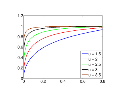
Figure 1: Function $G(\alpha,u)$ versus $\alpha$ for several values of $u$.

3.1 Minimax optimality of the average power

An upper bound for the minimax power of tests, with a given significant level $\alpha$, is provided in [JM13b] for sparse linear regression with Gaussian designs. Considering sample size scaling $n=\omega(s_{0}(\log p)^{2})$, the minimax bound [JM13b, Theorem 2.6] simplifies to the following bound for the optimal average power

$$\lim_{n\to\infty}\frac{1-\beta^{{\rm opt}}(\alpha;\mu)}{G(\alpha,\mu/\sigma_{\rm eff})}\leq 1\,,\quad\sigma_{\rm eff}=\frac{\sigma}{\sqrt{n\eta_{\Sigma,s_{0}}}}\,,$$ (18)

where

$$\eta_{\Sigma,s_{0}} \equiv\max_{i\in[p]}\min_{S}\Big{\{}\Sigma_{i|S}:\,S\subseteq[p]\backslash\{i\},|S|<s_{0}\Big{\}}\,,$$

$$\Sigma_{i|S} \equiv\Sigma_{ii}-\Sigma_{i,S}(\Sigma_{S,S})^{-1}\Sigma_{S,i}\,.$$

We compare our test to the optimal test by computing how much $\mu$ must be increased to achieve the minimax optimal average power. It follows from Eqs. (15) and (16) that $\mu$ must be increased to $\tilde{\mu}$, with the increase factor

$$\frac{\tilde{\mu}}{\mu}=\Big{(}\max_{i\in[p]}\sqrt{\Omega_{ii}}\Big{)}\sqrt{\eta_{\Sigma,s_{0}}}\leq\max_{i\in[p]}\sqrt{\Omega_{ii}\Sigma_{ii}}\leq\sqrt{\frac{\sigma_{\max}(\Sigma)}{\sigma_{\min}(\Sigma)}}\,.$$

Therefore, our test has nearly optimal average power for well-conditioned covariances and sample size scaling $n=\omega(s_{0}(\log p)^{2})$.

4 An estimator of the noise level

In this section we describe a consistent estimator $\widehat{\sigma}$ of the noise standard deviation $\sigma$, that is based on Proposition 2.1 and Theorem 2.3. After constructing $\widehat{\theta}^{u}$ as per Eq. (7), we let

$$z_{i}\equiv\frac{\sqrt{n}\,\widehat{\theta}^{u}_{i}}{[\widehat{\Omega}\widehat{\Sigma}\widehat{\Omega}^{\sf T}]^{1/2}_{ii}}\,.$$ (19)

According to Proposition 2.1 and Theorem 2.3, the entries $z_{i}$, $i\not\in S$ are approximately Gaussian, with mean $0$ and variance $\sigma^{2}$. This suggests to use the following robust estimator (a similar approach in a related context was proposed in [DMM09]).

Let $|z|$ be the vector of absolute values of $z$, i.e. $|z|=(|z_{1}|,|z_{2}|,\dots,|z_{p}|)$, and denote by $|z|_{(i)}$ its $i$-th entry in order of magnitude: $|z|_{(1)}\leq|z|_{(2)}\leq\dots\leq|z|_{(p)}$. We then set

$$\widehat{\sigma}=\frac{|z|_{(p/2)}}{\Phi^{-1}(3/4)}$$ (20)

The next corollary is an immediate consequence of Proposition 2.1 and Theorem 2.3 (see also Lemma 7.2).

Corollary 4.1.

Under the assumptions of Theorem 2.3, if further $s_{0}=o(p)$, we have $\widehat{\sigma}\to\sigma$ in probability.

5 Designs with sparse precision matrix

In Theorem 2.3 we posit existence of an estimator $\widehat{\Omega}$ for the precision matrix $\Omega$, such that $\|\widehat{\Omega}-\Omega\|_{\infty}=o(1/\sqrt{\log p})$. In case the precision matrix is sparse enough, then [vdGBR13] constructs such an estimator using the Lasso for the nodewise regression on the design ${\mathbf{X}}$. Formally, for $j\in[p]$, let

$$\hat{\gamma}_{j}=\underset{\gamma}{\arg\min}\,\frac{1}{2n}\|X_{j}-{\mathbf{X}}_{-j}\gamma\|_{2}^{2}+\lambda\|\gamma\|_{1}\,,$$

where ${\mathbf{X}}_{-j}$ is the sub-matrix obtained by removing the $j^{th}$ column. Also let

$$\widehat{C}=\begin{bmatrix}1&-\widehat{\gamma}_{1,2}&\cdots&-\widehat{\gamma}_{1,p}\\ -\widehat{\gamma}_{2,1}&1&\cdots&-\widehat{\gamma}_{1,p}\\ \vdots&\vdots&\ddots&\vdots\\ -\widehat{\gamma}_{p,1}&-\widehat{\gamma}_{p,2}&\cdots&1\end{bmatrix}\,,$$

with $\widehat{\gamma}_{j,k}$ being the $k$-th entry of $\widehat{\gamma}_{j}$, and let

$$\widehat{T}^{2}={\rm diag}(\widehat{\tau}_{1}^{2},\dotsc,\widehat{\tau}_{p}^{2}),\quad\widehat{\tau}_{j}^{2}=(X_{j}-{\mathbf{X}}_{-j}\widehat{\gamma}_{j})^{\sf T}X_{j}/n\,.$$

Then define $\widehat{\Omega}=\widehat{T}^{-2}\widehat{C}$.

Proposition 5.1 ([vdGBR13]).

Suppose that the whitened matrix ${\mathbf{X}}\Omega^{1/2}$ has i.i.d. sub-gaussian rows. Further, assume that the maximum number of non-zeros per row of $\Omega$ is $t_{0}=o(n/\log p)$, that $\sigma_{\max}(\Omega)=\sigma_{\rm min}(\Sigma)^{-1}=O(1)$ and that, for all $i\in[p]$, $\Sigma_{ii}=1$. Then, with high probability,

$$\|\widehat{\Omega}-\Omega\|_{\infty}=O(t_{0}\sqrt{\log p/n})\,.$$ (21)

Therefore, if $\Omega$ is sufficiently sparse, namely it has $t_{0}=o(\sqrt{n}/\log p)$ non-zeros per row, then Eq. (21) yields $\|\widehat{\Omega}-\Omega\|_{\infty}=o(1/\sqrt{\log p})$. Hence, the estimator $\widehat{\Omega}$ satisfies the conditions of Theorem 2.3 and 3.1.

6 Numerical experiments

We generated synthetic data from the linear model (1) with the choice of parameters $\sigma=1$, $n=240$ and $p=300$. The rows of the design matrix ${\mathbf{X}}$ are generated independently form distribution ${\sf N}(0,\Sigma)$. Here $\Omega=\Sigma^{-1}$ is a circulant matrix with $\Omega_{ii}=1$, $\Omega_{jk}=a$ for $j\neq k$, $|j-k|\leq b$, and zero everywhere else. (The difference between indices is understood modulo $p$.) The parameter $b$ controls the sparsity of the precision matrix and we take $a=1/b$ to ensure that $\Omega\succ 0$ (with $\sigma_{\min}(\Omega)>0.5$). For parameter vector $\theta_{0}$, we consider a subset $S\subseteq[p]$, with $|S|=s_{0}=30$, chosen uniformly at random, and set $\theta_{0,i}=0.1$ for $i\in S$ and zero everywhere else.

We evaluate the performance of our testing procedure (13) at significance level $\alpha=0.05$. The procedure is implemented in $R$ using glmnet-package that fits the Lasso solution for an entire path of regularization parameters $\lambda_{n}$. We then choose the value of $\lambda_{n}$ that has the minimum mean squares error, approximated by a $5$-fold cross validation.

We compare the performance of decision rule (13) to the testing method presented in [JM13a] for different values of $b$. (Recall that $b$ controls the sparsity of the precision matrix.) The results are reported in Table 1. The means and the standard deviations are obtained by testing over $20$ realizations of noise and the design matrix.

Interestingly, for small values of $b$ (very sparse precision matrices), the two methods perform often identically the same, and their performances differ slightly for moderate $b$. This is in agreement with the theoretical results that both methods asymptotically have nearly optimal minimax average power.

Letting $Z=(z_{i})_{i=1}^{p}$ with $z_{i}\equiv\sqrt{n}(\widehat{\theta}^{u}_{i}-\theta_{0,i})/[\widehat{\Omega}\widehat{\Sigma}\widehat{\Omega}]_{ii}^{1/2}$, in Fig. 3 we plot sample quantiles of $Z$ versus the quantiles of a standard normal distribution for one realization (with $b=75$). The linear trend of the plot clearly demonstrates that the empirical distribution of $Z$ is approximately normal, corroborating our theoretical results (Proposition 2.1 and Theorem 2.3).

Method	Type I err	Type I err	Avg. power	Avg. power
	(mean)	(std.)	(mean)	(std)
Present testing procedure $(b=5)$	0.0644	0.0060	0.5766	0.0387
Procedure of [JM13a] $(b=5)$	0.0644	0.0060	0.5766	0.0387
Present testing procedure $(b=25)$	0.0600	0.0074	0.5750	0.0445
Procedure of [JM13a] $(b=25)$	0.0600	0.0074	0.5750	0.0445
Present testing procedure $(b=50)$	0.0412	0.0061	0.5350	0.0383
Procedure of [JM13a] $(b=50)$	0.0468	0.0063	0.5416	0.0386
Present testing procedure $(b=75)$	0.0509	0.0075	0.4916	0.0334
Procedure of [JM13a] $(b=75)$	0.0507	0.0073	0.4900	0.0340
Present testing procedure $(b=100)$	0.0479	0.0067	0.5150	0.0310
Procedure of [JM13a] $(b=100)$	0.0618	0.0077	0.5416	0.0302

Table 1: Comparison between testing procedure (13) and procedure proposed in [JM13a] on the setup described in Section 6. The significance level is $\alpha=0.05$. The means and the standard deviations are obtained by testing over $20$ realizations.

7 Proofs

7.1 Proof of Theorem 2.3

Write $\Delta=\Delta^{(1)}+\Delta^{(2)}$ with

$$\Delta^{(1)}=\sqrt{n}(\Omega\widehat{\Sigma}-{\rm I})(\theta_{0}-\widehat{\theta})\,,\quad\Delta^{(2)}=\sqrt{n}(\widehat{\Omega}-\Omega)\widehat{\Sigma}(\theta_{0}-\widehat{\theta})\,.$$

Let $T\equiv{\rm supp}(\widehat{\theta})\cup{\rm supp}(\theta_{0})$. By Eq. (8), $|T|=O(s_{0})$ because $\phi_{\max}(n)\leq C$, $\kappa(s_{0},3)\geq 1/C$ for some constant $C<\infty$, with high probability. (This in turns follows from the assumption that $\sigma_{\rm max}(\Sigma)$, $\sigma_{\rm min}(\Sigma)$ are bounded above and below, using [RZ13].) Also, note that any set $A\subseteq[p]$ with $|A|\geq cs_{0}$ can be partitioned as $A=\cup_{\ell=1}^{L}A_{\ell}$ with $c\,s_{0}\leq|A_{\ell}|\leq 2c\,s_{0}$. If the claim holds for all $A_{\ell}$, then it follows for $A$ by summing these cases. We can therefore assume, without loss of generality, $c\,s_{0}\leq|A|\leq 2c\,s_{0}$.

(a) $b=5$

(b) $b=100$

Figure 2: Comparison between testing procedure (13) and the one proposed in [JM13a] for one realization.

Figure 3: Q-Q plot of $Z$ for one realization. Here $b=75$.

We first bound $\|\Delta^{(1)}_{A}\|_{2}$ using Hoeffding’s inequality. Note that

$$\Delta^{(1)}_{A}=\sqrt{n}(\Omega\widehat{\Sigma}-{\rm I})_{A,T}(\widehat{\theta}-\theta_{0})_{T}\,,$$

since ${\rm supp}(\widehat{\theta}-\theta_{0})\subseteq T$. Hence,

$$\|\Delta^{(1)}_{A}\|_{2}\leq\sqrt{n}\|(\Omega\widehat{\Sigma}-{\rm I})_{A,T}\|_{2}\|(\widehat{\theta}-\theta_{0})_{T}\|_{2}\,.$$ (22)

Let $R\equiv(\Omega\widehat{\Sigma}-{\rm I})_{A,T}$ and define ${\cal F}_{1}\equiv\{u\in S^{p-1}:\,{\rm supp}(u)\subseteq[A]\}$, ${\cal F}_{2}\equiv\{v\in S^{p-1}:\,{\rm supp}(v)\subseteq[T]\}$. We have

$$\|R\|_{2} =\underset{\begin{subarray}{c}u,v\\ \|u\|,\|v\|\leq 1\end{subarray}}{\sup}\langle u,Rv\rangle$$

$$=\underset{\begin{subarray}{c}u,v\\ \|u\|,\|v\|\leq 1\end{subarray}}{\sup}\Big{(}\langle u,\frac{1}{n}\sum_{i=1}^{n}(\Omega X_{i})_{A}(X_{i}^{\sf T})_{T}v\rangle-\langle u_{A},v_{T}\rangle\Big{)}$$

$$\leq\underset{u\in{\cal F}_{1},v\in{\cal F}_{2}}{\sup}\,\frac{1}{n}\sum_{i=1}^{n}\Big{(}\langle u,\Omega X_{i}\rangle\langle X_{i},v\rangle-\langle u,v\rangle\Big{)}\,.$$ (23)

Fix $u\in{\cal F}_{1}$ and $v\in{\cal F}_{2}$. Let $\xi_{i}\equiv\langle u,\Omega X_{i}\rangle\langle X_{i},v\rangle-\langle u,v\rangle$. The variables $\xi_{i}$ are independent and it is easy to see that ${\mathbb{E}}(\xi_{i})=0$. By [Ver12, Remark 5.18], we have

$$\|\xi_{i}\|_{\psi_{1}}\leq 2\|\langle u,\Omega X_{i}\rangle\langle X_{i},v\rangle\|_{\psi_{1}}\,.$$

Moreover, by Lemma C.1,

$$\|\langle u,\Omega X_{i}\rangle\langle X_{i},v\rangle\|_{\psi_{1}} \leq 2\|\langle u,\Omega X_{i}\rangle\|_{\psi_{2}}\|\langle X_{i},v\rangle\|_{\psi_{2}}$$

$$=\|\Omega^{1/2}u\|_{2}\|\Omega^{-1/2}v\|_{2}\|\Omega^{1/2}X_{i}\|_{\psi_{2}}^{2}$$

$$\leq\sqrt{\sigma_{\max}(\Sigma)/\sigma_{\min}(\Sigma)}\|\Omega^{1/2}X_{i}\|_{\psi_{2}}^{2}\,.$$

Hence, $\max_{i\in[n]}\|\xi_{i}\|_{\psi_{1}}\leq K$, for some constant $K$. Now, by applying Bernstein inequality for centered sub-exponential random variables [Ver12], for every $t\geq 0$, we have

$${\mathbb{P}}\bigg{(}\frac{1}{n}\sum_{i=1}^{n}\xi_{i}\geq t\Big{)}\leq 2\exp\bigg{[}-Cn\min\Big{(}\frac{t^{2}}{K^{2}},\frac{t}{K}\Big{)}\bigg{]}\,,$$

where $C>0$ is an absolute constant. Therefore, for any constant $c_{1}>0$, since $n=\omega(s_{0}\log p)$, we have

$${\mathbb{P}}\bigg{(}\frac{1}{n}\sum_{i=1}^{n}\xi_{i}\geq K\sqrt{\frac{c_{1}s_{0}\log p}{Cn}}\bigg{)}\leq p^{-c_{1}s_{0}}\,.$$ (24)

In order to bound the right hand side of Eq. (23), we use a ${\varepsilon}$-net argument. Clearly, ${\cal F}_{1}\cong S^{|A|-1}$ and ${\cal F}_{2}\cong S^{|T|-1}$ where $\cong$ denotes that the two objects are isometric. By [Ver12, Lemma 5.2], there exists a $\frac{1}{2}$-net ${\cal N}_{1}$ of $S^{|A|-1}$ (and hence of ${\cal F}_{1}$) with size at most $5^{|A|}$. Similarly there exists a $\frac{1}{2}$-net ${\cal N}_{2}$ of ${\cal F}_{2}$ of size at most $5^{|T|}$. Hence, using Eq. (24) and taking union bound over all vectors in ${\cal N}_{1}$ and ${\cal N}_{2}$ , we obtain

$$\underset{{u\in{\cal N}_{1}},{v\in{\cal N}_{2}}}{\sup}\frac{1}{n}\sum_{i=1}^{n}\langle u,(\Omega X_{i}X_{i}^{\sf T}-{\rm I})v\rangle\leq K\sqrt{\frac{c_{1}s_{0}\log p}{Cn}}\,,$$ (25)

with probability at least $1-5^{|A|+|T|}p^{-c_{1}s_{0}}$.

The last part of the argument is based on the following lemma, whose proof is deferred to Appendix D.

Lemma 7.1.

Let $M\in{\mathbb{R}}^{p\times p}$. Then,

$$\underset{u\in{\cal F}_{1},v\in{\cal F}_{2}}{\sup}\langle u,Mv\rangle\leq 4\underset{u\in{\cal N}_{1},v\in{\cal N}_{2}}{\sup}\langle u,Mv\rangle\,.$$

Employing Lemma 7.1 and bound (25) in Eq. (23), we arrive at

$$\|R\|_{2}\leq 4K\sqrt{\frac{c_{1}s_{0}\log p}{Cn}}\,,$$ (26)

with probability at least $1-5^{|A|+|T|}p^{-c_{1}s_{0}}$.

Finally, note that there are less than $p^{c^{\prime}s_{0}}$ subsets $A,T$, with $|T|\leq Cs_{0}$ and $|A|\leq 2cs_{0}$, for some constant $c^{\prime}>0$. Taking union bound over all these sets, we obtain that with high probability,

$$\|(\Omega\widehat{\Sigma}-{\rm I})_{A,T}\|_{2}\leq C\sqrt{s_{0}\log p/n}\,,$$

for all such sets $A,T$, where $C=C(c,C_{1},\sigma_{\max}(\Sigma),\sigma_{\min}(\Sigma))$ is a constant.

Now, plugging this bound and the bound (9) (recalling that $\kappa(s_{0},q,3)$ is bounded away from zero with high probability by [RZ13] because $\sigma_{\rm min}(\Sigma)$ is bounded away from zero) into Eq. (22), we get

$$\|\Delta^{(1)}_{A}\|_{2}\leq C\frac{\sigma s_{0}\log p}{\sqrt{n}}\,,$$ (27)

with $C=C(c,C_{1},\sigma_{\max}(\Sigma),\sigma_{\min}(\Sigma))$ a constant.

To bound $\|\Delta^{(2)}_{A}\|_{2}$, we bound each entry $\Delta^{(2)}_{i}$ separately:

$$|\Delta^{(2)}_{i}| \leq\sqrt{n}\|\widehat{\Omega}_{i,\cdot}-\Omega_{i,\cdot}\|_{1}\|\widehat{\Sigma}(\theta_{0}-\widehat{\theta})\|_{\infty}\,.$$ (28)

Note that the subgradient condition for optimization (3) reads

$$\Sigma(\widehat{\theta}-\theta_{0})={\mathbf{X}}^{\sf T}W/n+\lambda v(\widehat{\theta})\,,$$

with $v(\widehat{\theta})\in\partial\|\widehat{\theta}\|_{1}$. Thus $\|\Sigma(\widehat{\theta}-\theta_{0})\|_{\infty}=O(\sqrt{\log p/n})$, with high probability, for the choice of $\lambda=O(\sqrt{\log p/n})$. Therefore, Eq. (28) implies

$$\|\Delta^{(2)}\|_{\infty}=o(1)\,,$$ (29)

since by our assumption

$$\|\widehat{\Omega}-\Omega\|_{\infty}=\max_{i\in[p]}\|\widehat{\Omega}_{i,\cdot}-\Omega_{i,\cdot}\|_{1}=o(1/\sqrt{\log p})\,.$$

We are now ready to bound $\|\Delta_{A}\|_{2}^{2}/|A|$. By triangle inequality,

$$\|\Delta_{A}\|_{2}^{2}\leq 2\|\Delta^{(1)}_{A}\|_{2}^{2}+2\|\Delta^{(2)}\|_{2}^{2}\,.$$

Applying bounds (27) and (29), we obtain

$$\frac{\|\Delta_{A}\|_{2}^{2}}{|A|}\leq C\frac{\sigma^{2}s_{0}^{2}(\log p)^{2}}{n|A|}+o(1)\,.$$

This implies the thesis since$|A|\geq cs_{0}$ for some constant $c$.

7.2 Proof of Theorem 3.1

We begin with a lemma that lower bounds the variance of $\widehat{\theta}^{u}_{i}$.

Lemma 7.2.

Assume that the rows of ${\mathbf{X}}\Omega^{1/2}$ are subgaussian, i.e. $\|\Omega^{1/2}X_{1}\|_{\psi_{2}}<C$ for some constant $C$. Further assume that $1/C^{\prime}\leq\sigma_{\rm min}(\Sigma)\leq\sigma_{\rm max}(\Sigma)\leq C^{\prime}$, for some constant $C^{\prime}$. Finally assume that $\|\widehat{\Omega}-\Omega\|_{\infty}\leq 1/\sqrt{\log p}$ with probability at least $1-{\varepsilon}$.

Then for any constant $c_{0}>0$, there exist constants $c_{1},c_{2}>0$ such that

$${\mathbb{P}}\Big{(}\max_{i\in[p]}\big{|}[\widehat{\Omega}\widehat{\Sigma}\widehat{\Omega}^{\sf T}]_{ii}-\Omega_{ii}\big{|}\leq c_{0}\Big{)}\geq 1-c_{1}\,p^{2}\,e^{-c_{2}n}-{\varepsilon}\,.$$ (30)

Proof.

Fix $i\in[p]$, and let $v=\Omega^{\sf T}e_{i}$ be the $i$-th column of $\Omega$. Further let $\delta=(\Omega-\widehat{\Omega})^{\sf T}e_{i}$. Then,

$$[\widehat{\Omega}\widehat{\Sigma}\widehat{\Omega}^{\sf T}]_{ii} =(v-\delta)^{{\sf T}}\widehat{\Sigma}(v-\delta)=v^{{\sf T}}\widehat{\Sigma}v-2v^{{\sf T}}\widehat{\Sigma}\delta+\delta^{{\sf T}}\widehat{\Sigma}\delta\,.$$

Since $\widehat{\Sigma}\succeq 0$, we have

$$v^{\sf T}\widehat{\Sigma}\delta\leq\sqrt{(v^{\sf T}\widehat{\Sigma}v)(\delta^{\sf T}\widehat{\Sigma}\delta)}.$$

Consequently,

$$\Big{(}\sqrt{v^{{\sf T}}\widehat{\Sigma}v}-\sqrt{\delta^{{\sf T}}\widehat{\Sigma}\delta}\Big{)}^{2}\leq[\widehat{\Omega}\widehat{\Sigma}\widehat{\Omega}^{\sf T}]_{ii}\leq\Big{(}\sqrt{v^{{\sf T}}\widehat{\Sigma}v}+\sqrt{\delta^{{\sf T}}\widehat{\Sigma}\delta}\Big{)}^{2}\,.$$

Let ${\cal E}$ be the event that $\|\widehat{\Omega}-\Omega\|_{\infty}\leq 1/\sqrt{\log p}$. On ${\cal E}$, we have

$$\delta^{\sf T}\widehat{\Sigma}\delta=\sum_{i,j\in[p]}\widehat{\Sigma}_{ij}\delta_{i}\delta_{j}\leq|\widehat{\Sigma}|_{\infty}\|\delta\|_{1}^{2}\leq|\widehat{\Sigma}|_{\infty}\|\Omega-\widehat{\Omega}\|_{\infty}^{2}\leq\frac{|\widehat{\Sigma}|_{\infty}}{\log p}\,.$$

It is therefore sufficient to prove that $|v^{{\sf T}}\widehat{\Sigma}v-\Omega_{ii}|\leq c_{0}/2$ with probability at least $1-c_{1}\,e^{-c_{2}n}$, and $|\widehat{\Sigma}|_{\infty}<2$ with probability at least $1-c_{1}p^{2}\,e^{-c_{2}n}$. The claim then follows by union bound.

Consider first $v^{{\sf T}}\widehat{\Sigma}v$. We have ${\mathbb{E}}\{v^{{\sf T}}\widehat{\Sigma}v\}=[\Omega\Sigma\Omega]_{ii}=\Omega_{ii}$. Further

$$v^{{\sf T}}\widehat{\Sigma}v-{\mathbb{E}}(v^{{\sf T}}\widehat{\Sigma}v)=\frac{1}{n}\sum_{j=1}^{n}e_{i}^{{\sf T}}\Omega\big{[}X_{j}X_{j}^{{\sf T}}-{\mathbb{E}}(X_{j}X_{j}^{{\sf T}})\big{]}\Omega^{\sf T}e_{i}=\frac{1}{n}\sum_{j=1}^{n}\xi_{j}\,.$$ (31)

Here the $\xi_{j}$’s are i.i.d. sub-exponential with norm

$$\|\xi_{1}\|_{\psi_{1}}\leq 4\|\langle e_{i},\Omega X_{1}\rangle\|_{\psi_{2}}^{2}\leq 4C^{2}\|\Omega^{1/2}e_{i}\|_{2}^{2}\leq 4C^{2}\sigma_{\rm max}(\Omega)\leq 4C^{2}C^{\prime}\,.$$ (32)

The claim then follows by applying Bernstein inequality for sub-exponential random variables as in the proof in Section 7.1.

In order to bound $|\widehat{\Sigma}|_{\infty}$, we use

$${\mathbb{P}}\big{(}|\widehat{\Sigma}|_{\infty}\geq 2\big{)}\leq\sum_{i,j=1}^{p}{\mathbb{P}}\big{(}|\widehat{\Sigma}_{ij}|\geq 2\big{)}\leq\sum_{i,j=1}^{p}{\mathbb{P}}\big{(}|\widehat{\Sigma}_{ij}-{\mathbb{E}}\widehat{\Sigma}_{ij}|\geq 1\big{)}\,,$$ (33)

where the last inequality follows from ${\mathbb{E}}\widehat{\Sigma}_{ij}=\Sigma_{ij}\leq\sqrt{\Sigma_{ii}\Sigma_{jj}}=1$. Finally, the probability of $|\widehat{\Sigma}_{ij}-{\mathbb{E}}\widehat{\Sigma}_{ij}|\geq 1$ is bounded once again as above using Bernstein inequality. ∎

We next prove Eq. (14). For $i\in[p]$, let

$$A_{i}\equiv\frac{\sqrt{n}(\widehat{\theta}_{i}^{u}-\theta_{0,i})}{\widehat{\sigma}[\widehat{\Omega}\widehat{\Sigma}\widehat{\Omega}^{\sf T}]_{ii}^{1/2}}=\frac{\sigma}{\widehat{\sigma}}\widetilde{Z}_{i}+\frac{\Delta_{i}}{\widehat{\sigma}[\widehat{\Omega}\widehat{\Sigma}\widehat{\Omega}^{\sf T}]_{ii}^{1/2}}.$$

Invoking Proposition 2.1, $\widetilde{Z}_{i}|{\mathbf{X}}\sim{\sf N}(0,1)$. For any constant $b\geq 0$, we have

$$\sum_{i\in S_{0}^{c}}{\mathbb{P}}_{\theta_{0}}(|A_{i}|\geq b) \leq{\mathbb{E}}\Big{\{}\sum_{i\in S_{0}^{c}}{\mathbb{I}}\Big{(}|\widetilde{Z}_{i}|\geq\frac{\widehat{\sigma}}{\sigma}b-\frac{|\Delta_{i}|}{\sigma[\widehat{\Omega}\widehat{\Sigma}\widehat{\Omega}^{\sf T}]_{ii}^{1/2}}\Big{)}\Big{\}}$$

$$\leq{\mathbb{E}}\Big{\{}\sum_{i\in S_{0}^{c}\backslash{\cal C}_{n}({\varepsilon})}{\mathbb{I}}\Big{(}|\widetilde{Z}_{i}|\geq\frac{\widehat{\sigma}}{\sigma}b-\frac{|\Delta_{i}|}{\sigma[\widehat{\Omega}\widehat{\Sigma}\widehat{\Omega}^{\sf T}]_{ii}^{1/2}}\Big{)}+|{\cal C}_{n}({\varepsilon})|\Big{\}}\,.$$

By definition, $|\Delta_{i}|\leq{\varepsilon}$ for $i\in S_{0}^{c}\backslash{\cal C}_{n}({\varepsilon})$. Hence,

$$\frac{1}{p-s_{0}}\sum_{i\in S_{0}^{c}}{\mathbb{P}}_{\theta_{0}}(|A_{i}|\geq b)\leq\frac{1}{p-s_{0}}{\mathbb{E}}\Big{\{}\sum_{i\in S_{0}^{c}}{\mathbb{I}}\Big{(}|\widetilde{Z}_{i}|\geq\frac{\widehat{\sigma}}{\sigma}b-\frac{{\varepsilon}}{\sigma[\widehat{\Omega}\widehat{\Sigma}\widehat{\Omega}^{\sf T}]_{ii}^{1/2}}\Big{)}+|{\cal C}_{n}({\varepsilon})|\Big{\}}\,.$$ (34)

Let ${\cal G}\equiv{\cal G}(\delta,c_{0})$ be the following event:

$${\cal G}\equiv{\cal G}(\delta,c_{0})=\Big{\{}\max_{i\in[p]}\big{|}[\widehat{\Omega}\widehat{\Sigma}\widehat{\Omega}^{\sf T}]_{ii}-\Omega_{ii}\big{|}\leq c_{0},\,|\widehat{\sigma}/\sigma-1|\leq\delta\Big{\}}.$$

Then,

$${\mathbb{E}}\Big{\{}\sum_{i\in S_{0}^{c}}{\mathbb{I}}\Big{(}|\widetilde{Z}_{i}|\geq\frac{\widehat{\sigma}}{\sigma}b-\frac{{\varepsilon}}{\sigma[\widehat{\Omega}\widehat{\Sigma}\widehat{\Omega}^{\sf T}]_{ii}^{1/2}}\Big{)}\Big{\}} \leq{\mathbb{E}}\Big{\{}\Big{[}\sum_{i\in S_{0}^{c}}{\mathbb{I}}\Big{(}|\widetilde{Z}_{i}|\geq\frac{\widehat{\sigma}}{\sigma}b-\frac{{\varepsilon}}{\sigma[\widehat{\Omega}\widehat{\Sigma}\widehat{\Omega}^{\sf T}]_{ii}^{1/2}}\Big{)}\Big{]}\cdot{\mathbb{I}}({\cal G})\Big{\}}+{\mathbb{P}}({\cal G}^{c})$$

$$\leq{\mathbb{E}}\Big{\{}\Big{[}\sum_{i\in S_{0}^{c}}{\mathbb{I}}\Big{(}|\widetilde{Z}_{i}|\geq(1-\delta)b-\frac{{\varepsilon}}{\sigma\sqrt{\Omega_{ii}-c_{0}}}\Big{)}\Big{]}\cdot{\mathbb{I}}({\cal G})\Big{\}}+{\mathbb{P}}({\cal G}^{c})$$

$$\leq{\mathbb{E}}\Big{\{}\sum_{i\in S_{0}^{c}}{\mathbb{I}}\Big{(}|\widetilde{Z}_{i}|\geq(1-\delta)b-\frac{{\varepsilon}}{\sigma\sqrt{\Omega_{ii}-c_{0}}}\Big{)}\Big{\}}+{\mathbb{P}}({\cal G}^{c})\,.$$ (35)

Recalling that $\widetilde{Z}_{i}|{\mathbf{X}}\sim{\sf N}(0,1)$, the following holds for any $b^{\prime}\in{\mathbb{R}}$:

$${\mathbb{E}}({\mathbb{I}}(|\widetilde{Z}_{i}|\geq b^{\prime}))={\mathbb{E}}\{{\mathbb{P}}(|\widetilde{Z}_{i}|\geq b^{\prime}|{\mathbf{X}})\}=2(1-\Phi(b^{\prime}))\,.$$

Plugging in Eq. (35), we obtain

$$\underset{n\to\infty}{\lim\sup}\,\frac{1}{p-s_{0}}{\mathbb{E}}\Big{\{}\sum_{i\in S_{0}^{c}}{\mathbb{I}}\Big{(}|\widetilde{Z}_{i}|\geq\frac{\widehat{\sigma}}{\sigma}b-\frac{{\varepsilon}}{\sigma[\widehat{\Omega}\widehat{\Sigma}\widehat{\Omega}^{\sf T}]_{ii}^{1/2}}\Big{)}\Big{\}}\leq 2\Big{\{}1-\Phi\Big{(}(1-\delta)b-\frac{{\varepsilon}}{\sigma\sqrt{\Omega_{ii}-c_{0}}}\Big{)}\Big{\}}\,,$$ (36)

where in the last equality we used the fact that the event ${\cal G}$ holds with high probability, i.e., $\lim_{n\to\infty}{\mathbb{P}}({\cal G}^{c})=0$, as per Lemma 7.2.

Employing bound (36) in Eq. (34), we get

$$\underset{n\to\infty}{\lim\sup}\,\frac{1}{p-s_{0}}\sum_{i\in S_{0}^{c}}{\mathbb{P}}_{\theta_{0}}(|A_{i}|\geq b) \leq 2\Big{\{}1-\Phi\Big{(}(1-\delta)b-\frac{{\varepsilon}}{\sigma\sqrt{\Omega_{ii}-c_{0}}}\Big{)}\Big{\}}+\lim_{n\to\infty}{\mathbb{E}}\Big{(}\frac{|{\cal C}_{n}({\varepsilon})|}{p-s_{0}}\Big{)}$$

$$=2\Big{\{}1-\Phi\Big{(}(1-\delta)b-\frac{{\varepsilon}}{\sigma\sqrt{\Omega_{ii}-c_{0}}}\Big{)}\Big{\}}\,,$$

where the last step follows readily from Corollary 2.4. Since the above holds for all ${\varepsilon},\delta>0$, we obtain the following:

$$\underset{n\to\infty}{\lim\sup}\,\frac{1}{p-s_{0}}\sum_{i\in S_{0}^{c}}{\mathbb{P}}_{\theta_{0}}(|A_{i}|\geq b)\leq 2(1-\Phi(b))\,.$$ (37)

We are now ready to prove Eq. (14). For the decision rule given in Eq. (13), we have

$$\underset{n\to\infty}{\lim\sup}\,\frac{1}{p-s_{0}}\sum_{i\in S_{0}^{c}}{\mathbb{P}}_{\theta_{0}}(T_{i,{\mathbf{X}}}(y)=1)=\underset{n\to\infty}{\lim\sup}\,\frac{1}{p-s_{0}}\sum_{i\in S_{0}^{c}}{\mathbb{P}}_{\theta_{0}}(P_{i}\leq\alpha)$$

$$=\underset{n\to\infty}{\lim\sup}\,\frac{1}{p-s_{0}}\sum_{i\in S_{0}^{c}}{\mathbb{P}}_{\theta_{0}}\Big{(}\Phi^{-1}(1-\frac{\alpha}{2})\leq|A_{i}|\Big{)}\leq\alpha\,.$$

Here, the second equality follows from construction of $p$-values $P_{i}$ as per Eq.(12), and the fact that $\theta_{0,i}=0$, for $i\in S_{0}^{c}$; the inequality follows from Eq. (37), with $b=\Phi^{-1}(1-\alpha/2)$.

Eq. (15) can be proved in a similar way, as follows:

$$\frac{1}{s_{0}}\sum_{i\in S_{0}}{\mathbb{P}}_{\theta_{0}}(T_{i,{\mathbf{X}}}(y)=1) =\frac{1}{s_{0}}\sum_{i\in S_{0}}{\mathbb{P}}_{\theta_{0}}(P_{i}\leq\alpha)$$

$$=\frac{1}{s_{0}}\sum_{i\in S_{0}}{\mathbb{P}}_{\theta_{0}}\Big{(}\Phi^{-1}(1-\frac{\alpha}{2})\leq\frac{\sqrt{n}|\widehat{\theta}^{u}_{i}|}{\widehat{\sigma}[\widehat{\Omega}\widehat{\Sigma}\widehat{\Omega}^{\sf T}]_{ii}^{1/2}}\Big{)}$$

$$=\frac{1}{s_{0}}\sum_{i\in S_{0}}{\mathbb{P}}_{\theta_{0}}\Big{(}\Phi^{-1}(1-\frac{\alpha}{2})\leq\Big{|}\frac{\sigma}{\widehat{\sigma}}\widetilde{Z}_{i}+\frac{\sqrt{n}\theta_{0,i}+\Delta_{i}}{\widehat{\sigma}[\widehat{\Omega}\widehat{\Sigma}\widehat{\Omega}^{\sf T}]_{ii}^{1/2}}\Big{|}\Big{)}\,.$$

Define $\eta_{i}\equiv(\sqrt{n}\theta_{0,i}+\Delta_{i})/(\sigma[\widehat{\Omega}\widehat{\Sigma}\widehat{\Omega}^{\sf T}]_{ii}^{1/2})$. Rewriting the above identity we have

$$\frac{1}{s_{0}}\sum_{i\in S_{0}}{\mathbb{P}}_{\theta_{0}}(T_{i,{\mathbf{X}}}(y)=1) =\frac{1}{s_{0}}{\mathbb{E}}\Big{\{}\sum_{i\in S_{0}}{\mathbb{I}}\Big{(}\frac{\widehat{\sigma}}{\sigma}\Phi^{-1}(1-\frac{\alpha}{2})\leq|\widetilde{Z}_{i}+\eta_{i}|\Big{)}\Big{\}}$$

$$\geq\frac{1}{s_{0}}{\mathbb{E}}\Big{\{}\sum_{i\in S_{0}\backslash{\cal C}_{n}({\varepsilon})}{\mathbb{I}}\Big{(}\frac{\widehat{\sigma}}{\sigma}\Phi^{-1}(1-\frac{\alpha}{2})\leq|\widetilde{Z}_{i}+\eta_{i}|\Big{)}\Big{\}}\,.$$ (38)

By definition, $|\Delta_{i}|\leq{\varepsilon}$ for $i\in S_{0}\backslash{\cal C}_{n}({\varepsilon})$. Therefore, on the event ${\cal G}$ we have

$$|\eta_{i}|\geq\eta^{*}_{i}\equiv\frac{\sqrt{n}|\theta_{0,i}|-{\varepsilon}}{\sigma\sqrt{\Omega_{ii}+c_{0}}}\,,\quad\text{for }i\in S_{0}\backslash{\cal C}_{n}({\varepsilon})\,.$$

Moreover, $\widehat{\sigma}/\sigma\leq 1+\delta$. Fix arbitrary $\delta^{\prime}>0$ and define the event $\tilde{{\cal G}}$ as in the following

$$\tilde{{\cal G}}\equiv{\cal G}\cap\Big{\{}\frac{{\cal C}_{n}({\varepsilon})}{|s_{0}|}\leq\delta^{\prime}\Big{\}}\,.$$

Using Eq. (38), we have

$$\frac{1}{s_{0}}\sum_{i\in S_{0}}{\mathbb{P}}_{\theta_{0}}(T_{i,{\mathbf{X}}}(y)=1) \geq\frac{1}{s_{0}}{\mathbb{E}}\Big{\{}\Big{[}\sum_{i\in S_{0}\backslash{\cal C}_{n}({\varepsilon})}{\mathbb{I}}\Big{(}\frac{\widehat{\sigma}}{\sigma}\Phi^{-1}(1-\frac{\alpha}{2})\leq|\widetilde{Z}_{i}+\eta_{i}|\Big{)}\Big{]}\cdot{\mathbb{I}}(\tilde{{\cal G}})\Big{\}}-{\mathbb{P}}(\tilde{{\cal G}}^{c})$$

$$\geq\frac{1}{s_{0}}{\mathbb{E}}\Big{\{}\Big{[}\sum_{i\in S_{0}}{\mathbb{I}}\Big{(}\frac{\widehat{\sigma}}{\sigma}\Phi^{-1}(1-\frac{\alpha}{2})\leq|\widetilde{Z}_{i}+\eta_{i}|\Big{)}-|{\cal C}_{n}({\varepsilon})|\Big{]}\cdot{\mathbb{I}}(\tilde{{\cal G}})\Big{\}}-{\mathbb{P}}(\tilde{{\cal G}}^{c})$$

$$\geq\frac{1}{s_{0}}{\mathbb{E}}\Big{\{}\sum_{i\in S_{0}}{\mathbb{I}}\Big{(}(1+\delta)\Phi^{-1}(1-\frac{\alpha}{2})\leq|\widetilde{Z}_{i}+\eta^{*}_{i}|\Big{)}\Big{\}}-\delta^{\prime}-{\mathbb{P}}(\tilde{{\cal G}}^{c})\,,$$ (39)

where the last step follows from definition of event $\tilde{{\cal G}}$. Hence,

$$\underset{n\to\infty}{\lim\inf}\,\frac{1}{s_{0}(1-\beta^{*}(\theta_{0};n))}\Big{\{}\sum_{i\in S_{0}}{\mathbb{P}}_{\theta_{0}}(T_{i,{\mathbf{X}}}(y)=1)\Big{\}}$$

$$\geq\underset{n\to\infty}{\lim\inf}\,\frac{1}{s_{0}(1-\beta^{*}(\theta_{0};n))}\,{\mathbb{E}}\Big{\{}\sum_{i\in S_{0}}{\mathbb{I}}\Big{(}(1+\delta)\Phi^{-1}(1-\frac{\alpha}{2})\leq|\widetilde{Z}_{i}+\eta^{*}_{i}|\Big{)}\Big{\}}-\delta^{\prime}-\lim_{n\to\infty}{\mathbb{P}}(\tilde{{\cal G}}^{c})\,.$$

Given that $\widehat{\sigma}$ is a consistent estimator for $\sigma$, and using Lemma 7.2 and Corollary 2.4, the event $\tilde{{\cal G}}$ holds with high probability, i.e., $\lim_{n\to\infty}{\mathbb{P}}(\tilde{{\cal G}}^{c})=0$. Since the above bound holds for all $\delta^{\prime},{\varepsilon},c_{0}>0$, we get

$$\underset{n\to\infty}{\lim\inf}\,\frac{1}{s_{0}(1-\beta^{*}(\theta_{0};n))}\Big{\{}\sum_{i\in S_{0}}{\mathbb{P}}_{\theta_{0}}(T_{i,{\mathbf{X}}}(y)=1)\Big{\}}$$

$$\geq\underset{n\to\infty}{\lim\inf}\,\frac{1}{s_{0}(1-\beta^{*}(\theta_{0};n))}{\mathbb{E}}\Big{\{}\sum_{i\in S_{0}}{\mathbb{I}}\Big{(}\Phi^{-1}(1-\frac{\alpha}{2})\leq\Big{|}\widetilde{Z}_{i}+\frac{\sqrt{n}|\theta_{0,i}|}{\sigma\sqrt{\Omega_{ii}}}\Big{|}\Big{)}\Big{\}}$$

$$=\underset{n\to\infty}{\lim\inf}\,\frac{1}{(1-\beta^{*}(\theta_{0};n))}\Big{\{}\frac{1}{s_{0}}\sum_{i\in S_{0}}G\Big{(}\alpha,\frac{\sqrt{n}|\theta_{0,i}|}{\sigma\sqrt{\Omega_{ii}}}\Big{)}\Big{\}}=1\,.$$

The last step follows from definition of function $G(\cdot,\cdot)$, as per Eq. (17), and the fact that $\widetilde{Z}_{i}|{\mathbf{X}}\sim{\sf N}(0,1)$.

Appendix A Proof of Proposition 2.1

Plugging in $Y={\mathbf{X}}\theta_{0}+W$, we have

$$\sqrt{n}(\widehat{\theta}^{u}-\theta_{0})$$

$$=\sqrt{n}\Big{\{}\widehat{\theta}-\theta_{0}+\frac{1}{n}\widehat{\Omega}{\mathbf{X}}^{\sf T}W+\frac{1}{n}\widehat{\Omega}{\mathbf{X}}^{\sf T}{\mathbf{X}}(\theta_{0}-\widehat{\theta})\Big{\}}$$

$$=Z+\Delta\,,$$

where $Z=\widehat{\Omega}{\mathbf{X}}^{\sf T}W/\sqrt{n}$, and $\Delta=\sqrt{n}(\widehat{\Omega}\widehat{\Sigma}-{\rm I})(\theta_{0}-\widehat{\theta})$. Conditional on ${\mathbf{X}}$, we have $Z\sim{\sf N}(0,\sigma^{2}\widehat{\Omega}\widehat{\Sigma}\widehat{\Omega}^{\sf T})$, since $W\sim{\sf N}(0,\sigma^{2}{\rm I})$.

Appendix B Proof of Proposition 2.2

This proposition is a slightly improved version of Theorem 7.2 in [BRT09], in that we replace $\phi_{\max}(p)$ by $\phi_{\max}(n)$ in the bound on $\|\widehat{\theta}\|_{0}$. Here, we prove Eq. (8).

Let $\widehat{S}\equiv{\rm supp}(\widehat{\theta})$. Recall that the stationarity condition for the Lasso cost function reads ${\mathbf{X}}^{{\sf T}}(y-{\mathbf{X}}\widehat{\theta})=n\lambda\,v(\widehat{\theta})$, where $v(\widehat{\theta})\in\partial\|\widehat{\theta}\|_{1}$. Equivalently,

$$\frac{1}{n}{\mathbf{X}}^{{\sf T}}{\mathbf{X}}(\theta_{0}-\widehat{\theta})=\lambda\,v(\widehat{\theta})-\frac{1}{n}{\mathbf{X}}^{{\sf T}}w\,.$$

As proved in [BRT09], $\|{\mathbf{X}}^{\sf T}w\|_{\infty}\leq n\lambda/2$ with high probability. Thus for all $i\in\widehat{S}$

$$\left|\frac{1}{n}{\mathbf{X}}^{{\sf T}}{\mathbf{X}}(\theta_{0}-\widehat{\theta})\right|_{i}\geq\frac{\lambda}{2}\,.$$

Let ${\rm P}_{\widehat{S}}$ be the orthogonal projector in ${\mathbb{R}}^{p}$ on the subspace of vectors with support in $\widehat{S}$. Squaring and summing the last identity over $i\in\widehat{S}$, we obtain, for $h\equiv n^{-1/2}{\mathbf{X}}(\theta_{0}-\widehat{\theta})$,

$$|\widehat{S}| \leq\frac{4}{\lambda^{2}}\,\langle h,\frac{1}{n}{\mathbf{X}}{\rm P}_{\widehat{S}}{\mathbf{X}}^{{\sf T}}\,h\rangle$$

$$\leq\frac{4}{\lambda^{2}}\,\phi_{\rm max}(|\widehat{S}|)^{2}\|h\|_{2}^{2}\leq\frac{4\phi_{\rm max}(n)^{2}}{\lambda^{2}}\|h\|^{2}\,,$$

where the last inequality follows because $|\widehat{S}|\leq n$ by the fact that the columns of ${\mathbf{X}}$ are in generic positions (see e.g. [Tib13, Lemma 3]). By [BRT09, Theorem 6.2], we have $n^{-1}\|{\mathbf{X}}(\theta_{0}-\widehat{\theta})\|_{2}^{2}\leq 16\lambda^{2}s_{0}/\kappa(s_{0},3)^{2}$, whence the claim follows.

Appendix C Auxiliary lemmas

Lemma C.1.

For any two random variables $X$ and $Y$, we have

$$\|XY\|_{\psi_{1}}\leq 2\|X\|_{\psi_{2}}\|Y\|_{\psi_{2}}\,.$$

Proof.

By definition of sub-exponential and sub-gaussian norms, we write

$$\|XY\|_{\psi_{1}} =\underset{p\geq 1}{\sup}\,p^{-1}{\mathbb{E}}(|XY|^{p})^{1/p}$$

$$\leq\underset{p\geq 1}{\sup}\,p^{-1}{\mathbb{E}}(|X|^{2p})^{1/2p}{\mathbb{E}}(|Y|^{2p})^{1/2p}$$

$$\leq 2\Big{(}\underset{q\geq 2}{\sup}\,q^{-1/2}{\mathbb{E}}(|X|^{q})^{1/q}\Big{)}\Big{(}\underset{q\geq 2}{\sup}\,q^{-1/2}{\mathbb{E}}(|Y|^{q})^{1/q}\Big{)}$$

$$\leq 2\|X\|_{\psi_{2}}\|Y\|_{\psi_{2}}\,.$$

Here, the first inequality follows from Cauchy-Schwartz inequality. ∎

Appendix D Proof of Lemma 7.1

Each vector $u\in{\cal F}_{1}$ can be written as $u=\sum_{i=0}^{\infty}2^{-i}u_{i}$, where $u_{i}\in{\cal N}_{1}$. Similarly, each vector $v\in{\cal F}_{2}$ can be written as $v=\sum_{j=0}^{\infty}2^{-j}v_{j}$. Therefore,

$$\langle u,Mv\rangle=\sum_{i,j=0}^{\infty}2^{-i-j}\langle u_{i},Mv_{j}\rangle\leq 4\underset{u^{\prime}\in{\cal N}_{1},v^{\prime}\in{\cal N}_{2}}{\sup}\langle u^{\prime},Mv^{\prime}\rangle\,.$$

The result follows.

References

- [BCW11] Alexandre Belloni, Victor Chernozhukov, and Lie Wang, Square-root lasso: pivotal recovery of sparse signals via conic programming, Biometrika 98 (2011), no. 4, 791–806.
- [BRT09] P. J. Bickel, Y. Ritov, and A. B. Tsybakov, Simultaneous analysis of Lasso and Dantzig selector, Annals of Statistics 37 (2009), 1705–1732.
- [Büh12] P. Bühlmann, Statistical significance in high-dimensional linear models, arXiv:1202.1377, 2012.
- [BvdG11] Peter Bühlmann and Sara van de Geer, Statistics for high-dimensional data, Springer-Verlag, 2011.
- [CD95] S.S. Chen and D.L. Donoho, Examples of basis pursuit, Proceedings of Wavelet Applications in Signal and Image Processing III (San Diego, CA), 1995.
- [CT05] E. J. Candés and T. Tao, Decoding by linear programming, IEEE Trans. on Inform. Theory 51 (2005), 4203–4215.
- [CT07] E. Candés and T. Tao, The Dantzig selector: statistical estimation when p is much larger than n, Annals of Statistics 35 (2007), 2313–2351.
- [DMM09] D. L. Donoho, A. Maleki, and A. Montanari, Message Passing Algorithms for Compressed Sensing, Proceedings of the National Academy of Sciences 106 (2009), 18914–18919.
- [DT05] D. L. Donoho and J. Tanner, Neighborliness of randomly-projected simplices in high dimensions, Proceedings of the National Academy of Sciences 102 (2005), no. 27, 9452–9457.
- [JM13a] Adel Javanmard and Andrea Montanari, Confidence Intervals and Hypothesis Testing for High-Dimensional Regression, arXiv:1306.3171, 2013.
- [JM13b] , Hypothesis testing in high-dimensional regression under the gaussian random design model: Asymptotic theory, arXiv:1301.4240, 2013.
- [MB06] N. Meinshausen and P. Bühlmann, High-dimensional graphs and variable selection with the lasso, Ann. Statist. 34 (2006), 1436–1462.
- [RZ13] Mark Rudelson and Shuheng Zhou, Reconstruction from anisotropic random measurements, IEEE Transactions on Information Theory 59 (2013), no. 6, 3434–3447.
- [SZ12] Tingni Sun and Cun-Hui Zhang, Scaled sparse linear regression, Biometrika 99 (2012), no. 4, 879–898.
- [Tib96] R. Tibshirani, Regression shrinkage and selection with the Lasso, J. Royal. Statist. Soc B 58 (1996), 267–288.
- [Tib13] Ryan J. Tibshirani, The lasso problem and uniqueness, Electronic Journal of Statistics 7 (2013), 1456–1490.
- [vdGBR13] S. van de Geer, P. Bühlmann, and Y. Ritov, On asymptotically optimal confidence regions and tests for high-dimensional models, arXiv:1303.0518, 2013.
- [Ver12] R. Vershynin, Introduction to the non-asymptotic analysis of random matrices, Compressed Sensing: Theory and Applications (Y.C. Eldar and G. Kutyniok, eds.), Cambridge University Press, 2012, pp. 210–268.
- [Wai09] M.J. Wainwright, Sharp thresholds for high-dimensional and noisy sparsity recovery using -constrained quadratic programming, IEEE Trans. on Inform. Theory 55 (2009), 2183–2202.
- [ZZ11] C.-H. Zhang and S.S. Zhang, Confidence Intervals for Low-Dimensional Parameters in High-Dimensional Linear Models, arXiv:1110.2563, 2011.