Abstract

We study the bispectrum of the matter density perturbations induced by the large scale structure formation in the most general second-order scalar-tensor theory that may possess the Vainshtein mechanism as a screening mechanism. On the basis of the standard perturbation theory, we derive the bispectrum being expressed by a kernel of the second order of the density perturbations. We find that the kernel at the leading order is characterized by one parameter, which is determined by the solutions of the linear density perturbations, the Hubble parameter and the other function specifying nonlinear interactions. This does not allow for varied behavior in the bispectrum of the matter density perturbations in the most general second-order scalar-tensor theory equipped with the Vainshtein mechanism. We exemplify the typical behavior of the bispectrum in a kinetic gravity braiding model.

I Introduction

Modified gravity models attract interests of researchers as an alternative to explain the cosmic accelerated expansion of the universe without introducing the cosmological constant HuSawicki ; Starobinsky ; Tsujikawafr ; Nojirib ; DGP2 ; Song ; Maartens ; KM ; MassiveG ; MassiveG2 ; MassiveG3 ; HA . The most general second-order scalar-tensor theory was constructed by Horndeski Horndeski for the first time, and it was rediscovered in DGSZ as a generalization of the galileon theories Koba ; GC ; SAUGC ; ELCP ; CEGH ; GGC ; GBDT ; DPGMGT ; CG ; GGIR ; MGALG ; CCGF ; OCG ; CSTOG ; FeliceTsujikawa ; Deffayet ; DDEF ; GALMG ; RFFGM ; SSSDBI ; DBIGR . In addition to the possibility of constructing cosmological models with an accelerated expansion, it possesses the following interesting features. The equation of motion are the second order differential equation. Then, an additional degree of freedom is not introduced, which is advantageous to avoid the appearance of ghosts. Furthermore, the galileon theory is endowed with the Vainshtein mechanism GALMG , which is a screening mechanism useful to evade the local gravity constraints. In the most general second-order scalar-tensor theory, the Vainshtein mechanism may work depending on the model parameters (e.g., KKY ; Kase ; Narikawa ).

The results of the Planck satellite have shown that the primordial perturbations obey almost the Gaussian statistics Planckresults . Even if the initial perturbations were completely Gaussian, the non-Gaussian nature in the density perturbations is induced in the large scale structure formation through the nonlinear fluid equations under the influence of the gravitational force. The bispectrum is often used to characterize the nonlinear and non-Gaussian nature in the density perturbations (e.g., Bispectrum1 ; Bispectrum2 ; Bispectrum3 ; BMR1 ; BMR2 ). Recently, bispectrum and nonlinear features in the structure formation in the galileon models have been investigated KTH ; Barreira ; BLi ; Wyman ; Bellini ; Emilio ; kgb . In the present paper, we focus our investigation on the bispectrum in the most general second-order scalar-tensor theory in order to illuminate characteristic features in a wide class of modified gravity models, regarding it as an effective theory. An advantage of such a general theory is that we can discuss general features of a wide class of modified gravity models, which is useful to forecast their detectability in future large surveys.

In the present paper, we consider the bispectrum in the matter density perturbations which is induced in the large scale structure formation after the matter dominated epoch. We present an expression of the bispectrum in the most general second-order scalar-tensor theory based on the standard density perturbation theory, which is written in term of a kernel of the second order of perturbations. We find that the kernel is characterized by only one parameter, which is determined by the solutions of the linear density perturbations, the Hubble parameter, and the other function of the background universe that describes the nonlinear interactions. This paper is organized as follows: In section 2, we apply the standard perturbation theory to the most general second-order scalar-tensor theory that may possess the Vainshtein mechanism, and find the solution of the second-order of density perturbations. In section 3, we present the expression of the bispectrum of the density perturbations, and investigate the influence of the modification of gravity. The results are applied to a simple kinetic gravity braiding model in section 4. Section 5 is devoted to summary and conclusions.

II Formulation

We consider the most general second-order scalar-tensor theory on the expanding universe background. The action is given by

$$S=\int d^{4}x\sqrt{-g}\left({\cal L}_{\rm GG}+{\cal L}_{\rm m}\right),$$ (1)

where we defined

$${\cal L}_{\rm GG} = K(\phi,X)-G_{3}(\phi,X)\Box\phi+G_{4}(\phi,X)R+G_{4X}\left[(\Box\phi)^{2}-(\nabla_{\mu}\nabla_{\nu}\phi)^{2}\right]$$ (2)

$$+G_{5}(\phi,X)G_{\mu\nu}\nabla^{\mu}\nabla^{\nu}\phi-\frac{1}{6}G_{5X}\bigl{[}(\Box\phi)^{3}-3\Box\phi(\nabla_{\mu}\nabla_{\nu}\phi)^{2}+2(\nabla_{\mu}\nabla_{\nu}\phi)^{3}\bigr{]},$$

with four arbitrary functions, $K,G_{3},G_{4},$ and $G_{5}$, of $\phi$ and $X:=-(\partial\phi)^{2}/2$, $G_{iX}$ stands for $\partial G_{i}/\partial X$, $R$ is the Ricci scalar, $G_{\mu\nu}$ is the Einstein tensor, and ${\cal L}_{\rm m}$ is the matter Lagrangian, which is assumed to be minimally coupled to gravity. This theory is found in DGSZ as a generalization of the galileon theory, but the equivalence with the Horndeski’s theory is shown in Koba . We consider a spatially flat expanding universe and the metric perturbations in the Newtonian gauge, whose line element is written as

$$ds^{2}=-(1+2\Phi)dt^{2}+a^{2}(1-2\Psi)d\mathbf{x}^{2}.$$ (3)

We define the scalar field with perturbations by

$$\phi \to \phi(t)+\delta\phi(t,\mathbf{x}),$$ (4)

with which we introduce $Q:=H{\delta\phi}/{\dot{\phi}}$.

We consider the case that the Vainshtein mechanism may work as a screening mechanism. The basic equations for the cosmological density perturbations are derived in Ref. KKY . Here we briefly review the method and the results (see KKY for details). The basic equations of the gravitational and scalar fields are derived on the basis of the quasi-static approximation of the subhorizon scales. The models that the Vainshtein mechanism may work can be found as follows. The equations are derived by keeping the leading terms schematically written as $(\partial\partial Y)^{n}$, with $n\geq 1$, where $\partial$ denotes a spatial derivative and $Y$ does any of $\Phi$, $\Psi$ or $Q$. Such terms make a leading contribution of the order $(L_{\rm H}^{2}\partial\partial Y)^{n}$, where $L_{\rm H}$ is a typical horizon length scale. According to Ref. KKY , from the gravitational field equation, we have

$$\nabla^{2}\left({\cal F}_{T}\Psi-{\cal G}_{T}\Phi-A_{1}Q\right)=\frac{B_{1}}{2a^{2}H^{2}}{\cal Q}^{(2)}+\frac{B_{3}}{a^{2}H^{2}}\left(\nabla^{2}\Phi\nabla^{2}Q-\partial_{i}\partial_{j}\Phi\partial^{i}\partial^{j}Q\right),$$ (5)

$${\cal G}_{T}\nabla^{2}\Psi=\frac{a^{2}}{2}\rho_{\rm m}\delta-A_{2}\nabla^{2}Q-\frac{B_{2}}{2a^{2}H^{2}}{\cal Q}^{(2)}-\frac{B_{3}}{a^{2}H^{2}}\left(\nabla^{2}\Psi\nabla^{2}Q-\partial_{i}\partial_{j}\Psi\partial^{i}\partial^{j}Q\right)-\frac{C_{1}}{3a^{4}H^{4}}{\cal Q}^{(3)},$$ (6)

where $\rho_{\rm m}$ is the matter density, $\delta$ is the matter density contrast, and we defined

$${\cal Q}^{(2)}:=\left(\nabla^{2}Q\right)^{2}-\left(\partial_{i}\partial_{j}Q\right)^{2},$$ (7)

$${\cal Q}^{(3)}:=\left(\nabla^{2}Q\right)^{3}-3\nabla^{2}Q\left(\partial_{i}\partial_{j}Q\right)^{2}+2\left(\partial_{i}\partial_{j}Q\right)^{3}.$$ (8)

From the equation of motion of the scalar field, we have

$$A_{0}\nabla^{2}Q-A_{1}\nabla^{2}\Psi-A_{2}\nabla^{2}\Phi+\frac{B_{0}}{a^{2}H^{2}}{\cal Q}^{(2)}-\frac{B_{1}}{a^{2}H^{2}}\left(\nabla^{2}\Psi\nabla^{2}Q-\partial_{i}\partial_{j}\Psi\partial^{i}\partial^{j}Q\right)$$

$$-\frac{B_{2}}{a^{2}H^{2}}\left(\nabla^{2}\Phi\nabla^{2}Q-\partial_{i}\partial_{j}\Phi\partial^{i}\partial^{j}Q\right)-\frac{B_{3}}{a^{2}H^{2}}\left(\nabla^{2}\Phi\nabla^{2}\Psi-\partial_{i}\partial_{j}\Phi\partial^{i}\partial^{j}\Psi\right)$$

$$-\frac{C_{0}}{a^{4}H^{4}}{\cal Q}^{(3)}-\frac{C_{1}}{a^{4}H^{4}}{\cal U}^{(3)}=0,$$ (9)

where we defined

$${\cal U}^{(3)} := {\cal Q}^{(2)}\nabla^{2}\Phi-2\nabla^{2}Q\partial_{i}\partial_{j}Q\partial^{i}\partial^{j}\Phi+2\partial_{i}\partial_{j}Q\partial^{j}\partial^{k}Q\partial_{k}\partial^{i}\Phi.$$ (10)

The coefficients such as ${\cal F}_{T}$, $A_{1}$, $B_{1}$, etc., that appear in the field equations here and hereafter are defined in Appendix A. $A_{i},B_{i},C_{i}$ are the coefficients of the linear, quadratic and cubic terms of $\Psi$, $\Phi$, $Q$, respectively.

Equations for the matter density contrast $\delta$ and the velocity field $u^{i}$ are given by

$${\partial\delta(t,{\bf x})\over\partial t}+{1\over a}\partial_{i}[(1+\delta(t,{\bf x}))u^{i}(t,{\bf x})]=0,$$ (11)

$${\partial u^{i}(t,{\bf x})\over\partial t}+{\dot{a}\over a}u^{i}(t,{\bf x})+{1\over a}u^{j}(t,{\bf x})\partial_{j}u^{i}(t,{\bf x})=-{1\over a}\partial^{i}\Phi(t,{\bf x}),$$ (12)

where the dot denotes the differentiation with respect to $t$. The effect of the gravity comes through the gravitational potential $\Phi$, which is determined by the above equations (5), (6) and (9). Here, we only consider the scalar mode of the density perturbations, then we introduce a scalar function by $\theta\equiv\nabla{\bf u}/(aH)$. Now we define the Fourier expansion as for the quantities $\delta$ and $\theta$,

$$\delta(t,{\bf x})={1\over(2\pi)^{3}}\int d^{3}p\delta(t,{\bf p})e^{i{\bf p}\cdot{\bf x}},$$ (13)

$$u^{j}(t,{\bf x})={1\over(2\pi)^{3}}\int d^{3}p{-ip^{j}\over p^{2}}aH\theta(t,{\bf p})e^{i{\bf p}\cdot{\bf x}}.$$ (14)

The Fourier expansion for $\Phi$, $\Psi$ and $Q$ is defined in the similar way to (13). Then, (5) and (6) yield

$$-p^{2}\left({\cal F}_{T}\Psi(t,{\bf p})-{\cal G}_{T}\Phi(t,{\bf p})-A_{1}Q(t,{\bf p})\right)=\frac{B_{1}}{2a^{2}H^{2}}\Gamma[t,{\bf p};Q,Q]+\frac{B_{3}}{a^{2}H^{2}}\Gamma[t,{\bf p};Q,\Phi]$$ (15)

$$-p^{2}({\cal G}_{T}\Psi(t,{\bf p})+A_{2}Q(t,{\bf p}))-\frac{a^{2}}{2}\rho_{\rm m}\delta(t,{\bf p})=-\frac{B_{2}}{2a^{2}H^{2}}\Gamma[t,{\bf p};Q,Q]-\frac{B_{3}}{a^{2}H^{2}}\Gamma[t,{\bf p};Q,\Psi]$$

$$~{}~{}~{}~{}~{}~{}~{}-\frac{C_{1}}{3a^{4}H^{4}}{1\over(2\pi)^{6}}\int d{\bf k}_{1}d{\bf k}_{2}d{\bf k}_{3}\delta^{(3)}({\bf k}_{1}+{\bf k}_{2}+{\bf k}_{3}-{\bf p})$$

$$~{}~{}~{}~{}~{}~{}~{}\times\biggl{[}-k_{1}^{2}k_{2}^{2}k_{3}^{2}+3k_{1}^{2}({\bf k}_{2}\cdot{\bf k}_{3})^{2}-2({\bf k}_{1}\cdot{\bf k}_{2})({\bf k}_{2}\cdot{\bf k}_{3})({\bf k}_{3}\cdot{\bf k}_{1})\biggr{]}Q(t,{\bf k}_{1})Q(t,{\bf k}_{2})Q(t,{\bf k}_{3}),$$ (16)

where we defined

$$\Gamma[t,{\bf p};Y,Z]={1\over(2\pi)^{3}}\int d{\bf k}_{1}d{\bf k}_{2}\delta^{(3)}({\bf k}_{1}+{\bf k}_{2}-{\bf p})\left(k_{1}^{2}k_{2}^{2}-({\bf k}_{1}\cdot{\bf k}_{2})^{2}\right)Y(t,{\bf k}_{1})Z(t,{\bf k}_{2}),$$ (17)

where $Y$ and $Z$ denote any of $Q$, $\Phi$, or $\Psi$. Eq. (9) leads to

$$-p^{2}(A_{0}Q(t,{\bf p})-A_{1}\Psi(t,{\bf p})-A_{2}\Phi(t,{\bf p}))$$

$$~{}~{}~{}~{}=-\frac{B_{0}}{a^{2}H^{2}}\Gamma[t,{\bf p};Q,Q]+\frac{B_{1}}{a^{2}H^{2}}\Gamma[t,{\bf p};Q,\Psi]+\frac{B_{2}}{a^{2}H^{2}}\Gamma[t,{\bf p};Q,\Phi]+\frac{B_{3}}{a^{2}H^{2}}\Gamma[t,{\bf p};\Psi,\Phi]$$

$$~{}~{}~{}~{}+\frac{C_{0}}{a^{4}H^{4}}{1\over(2\pi)^{6}}\int d{\bf k}_{1}d{\bf k}_{2}d{\bf k}_{3}\delta^{(3)}({\bf k}_{1}+{\bf k}_{2}+{\bf k}_{3}-{\bf p})\biggl{[}-k_{1}^{2}k_{2}^{2}k_{3}^{2}+3k_{1}^{2}({\bf k}_{2}\cdot{\bf k}_{3})^{2}$$

$$~{}~{}~{}~{}\hskip 2.84544pt-2({\bf k}_{1}\cdot{\bf k}_{2})({\bf k}_{2}\cdot{\bf k}_{3})({\bf k}_{3}\cdot{\bf k}_{1})\biggr{]}Q(t,{\bf k}_{1})Q(t,{\bf k}_{2})Q(t,{\bf k}_{3})$$

$$~{}~{}~{}~{}+\frac{C_{1}}{a^{4}H^{4}}{1\over(2\pi)^{6}}\int d{\bf k}_{1}d{\bf k}_{2}d{\bf k}_{3}\delta^{(3)}({\bf k}_{1}+{\bf k}_{2}+{\bf k}_{3}-{\bf p})\biggl{[}-k_{1}^{2}k_{2}^{2}k_{3}^{2}+({\bf k}_{1}\cdot{\bf k}_{2})^{2}k_{3}^{2}$$

$$~{}~{}~{}~{}\hskip 2.84544pt+2k_{1}^{2}({\bf k}_{2}\cdot{\bf k}_{3})^{2}-2({\bf k}_{1}\cdot{\bf k}_{2})({\bf k}_{2}\cdot{\bf k}_{3})({\bf k}_{3}\cdot{\bf k}_{1})\biggr{]}Q(t,{\bf k}_{1})Q(t,{\bf k}_{2})\Phi(t,{\bf k}_{3}).$$ (18)

Equations (11) and (12) are rephrased as

$${1\over H}{\partial\delta(t,{\bf p})\over\partial t}+\theta(t,{\bf p})=-{1\over(2\pi)^{3}}\int d{\bf k}_{1}d{\bf k}_{2}\delta^{(3)}({\bf k}_{1}+{\bf k}_{2}-{\bf p})\left(1+{{\bf k}_{1}\cdot{\bf k}_{2}\over k_{2}^{2}}\right)\delta(t,{\bf k}_{1})\theta(t,{\bf k}_{2}),$$ (19)

$${1\over H}{\partial\theta(t,{\bf p})\over\partial t}+\left(2+{\dot{H}\over H^{2}}\right)\theta(t,{\bf p})-{p^{2}\over a^{2}H^{2}}\Phi(t,{\bf p})$$

$$\hskip 28.45274pt=-{1\over 2}{1\over(2\pi)^{3}}\int d{\bf k}_{1}d{\bf k}_{2}\delta^{(3)}({\bf k}_{1}+{\bf k}_{2}-{\bf p})\left({({\bf k}_{1}\cdot{\bf k}_{2})|{\bf k}_{1}+{\bf k}_{2}|^{2}\over k_{1}^{2}k_{2}^{2}}\right)\theta(t,{\bf k}_{1})\theta(t,{\bf k}_{2}).$$ (20)

We find the solution in terms of the perturbative expansion, which can be written in a form

$$Y(t,{\bf p}) = \sum_{n=1}Y_{n}(t,{\bf p}),$$ (21)

where $Y$ denotes $\delta,\theta,\Psi,\Phi$, or $Q$, and $Y_{n}$ denotes the $n$-th order solution of the expansion.

Now we start from the first order equations, which can be easily solved as follows. From equations (15), (16), and (18), we have

$${\cal F}_{T}p^{2}\Psi_{1}(t,{\bf p})-{\cal G}_{T}p^{2}\Phi_{1}(t,{\bf p})-A_{1}p^{2}Q_{1}(t,{\bf p})=0,$$ (22)

$${\cal G}_{T}p^{2}\Psi_{1}(t,{\bf p})+A_{2}p^{2}Q_{1}(t,{\bf p})=-{a^{2}\over 2}\rho_{\rm m}\delta_{1}(t,{\bf p}),$$ (23)

$$A_{0}p^{2}Q_{1}(t,{\bf p})-A_{1}p^{2}\Psi_{1}(t,{\bf p})-A_{2}p^{2}\Phi_{1}(t,{\bf p})=0,$$ (24)

which give the solutions

$$\Phi_{1}(t,{\bf p}) = -{a^{2}\rho_{\rm m}{\cal R}(t)\over p^{2}{\cal Z}(t)}\delta_{1}(t,{\bf p}),$$ (25)

$$\Psi_{1}(t,{\bf p}) = -{a^{2}\rho_{\rm m}{\cal S}(t)\over p^{2}{\cal Z}(t)}\delta_{1}(t,{\bf p}),$$ (26)

$$Q_{1}(t,{\bf p}) = -{a^{2}\rho_{\rm m}{\cal T}(t)\over p^{2}{\cal Z}(t)}\delta_{1}(t,{\bf p}),$$ (27)

where we defined

$${\cal R}(t)=A_{0}{\cal F}_{T}-A_{1}^{2},$$ (28)

$${\cal S}(t)=A_{0}{\cal G}_{T}+A_{1}A_{2},$$ (29)

$${\cal T}(t)=A_{1}{\cal G}_{T}+A_{2}{\cal F}_{T},$$ (30)

$${\cal Z}(t)=2(A_{0}{\cal G}_{T}^{2}+2A_{1}A_{2}{\cal G}_{T}+A_{2}^{2}{\cal F}_{T}).$$ (31)

The first order equation of (19) is

$$\theta_{1}(t,{\bf p})=-{1\over H}{\partial\delta_{1}(t,{\bf p})\over\partial t}.$$ (32)

Substituting (32) and (25) into the first order equation of (20), we have

$${\partial^{2}\delta_{1}(t,{\bf p})\over\partial t^{2}}+2H{\partial\delta_{1}(t,{\bf p})\over\partial t}+L(t)\delta_{1}(t,{\bf p})=0,$$ (33)

where we defined

$$L(t)=-{(A_{0}{\cal F}_{T}-A_{1}^{2})\rho_{\rm m}\over 2(A_{0}{\cal G}_{T}^{2}+2A_{1}A_{2}{\cal G}_{T}+A_{2}^{2}{\cal F}_{T})}.$$ (34)

This second rank differential equation has the growing mode solution $D_{+}(t)$ and the decaying mode solution $D_{-}(t)$. Neglecting the decaying mode solution, we write the first order solution,

$$\delta_{1}(t,{\bf p})=D_{+}(t)\delta_{\rm L}({\bf p}),$$ (35)

where $\delta_{\rm L}({\bf p})$ is a constant, which is determined by the initial density fluctuations. We assume that $\delta_{\rm L}({\bf p})$ obeys the Gaussian random statistics. Here we adopt the normalization $D_{+}(a)=a$ at $a\ll 1$. The first order solutions for the other quantities can be expressed in terms of $\delta_{1}(t,{\bf p})$.

Then, we consider the second order equations of the perturbative expansion. From (15), (16) and (18), the second order equations are

$$-p^{2}\left({\cal F}_{T}\Psi_{2}(t,{\bf p})-{\cal G}_{T}\Phi_{2}(t,{\bf p})-A_{1}Q_{2}(t,{\bf p})\right)=\frac{B_{1}}{2a^{2}H^{2}}\Gamma[t,{\bf p};Q_{1},Q_{1}]+\frac{B_{3}}{a^{2}H^{2}}\Gamma[t,{\bf p};Q_{1},\Phi_{1}],$$ (36)

$$-p^{2}({\cal G}_{T}\Psi_{2}(t,{\bf p})+A_{2}Q_{2}(t,{\bf p})=\frac{a^{2}}{2}\rho_{\rm m}\delta_{2}(t,{\bf p})-\frac{B_{2}}{2a^{2}H^{2}}\Gamma[t,{\bf p};Q_{1},Q_{1}]-\frac{B_{3}}{a^{2}H^{2}}\Gamma[t,{\bf p};Q_{1},\Psi_{1}],$$ (37)

$$-p^{2}(A_{0}Q_{2}(t,{\bf p})-A_{1}\Psi_{2}(t,{\bf p})-A_{2}\Phi_{2}(t,{\bf p}))$$

$$~{}~{}~{}~{}=-\frac{B_{0}}{a^{2}H^{2}}\Gamma[t,{\bf p};Q_{1},Q_{1}]+\frac{B_{1}}{a^{2}H^{2}}\Gamma[t,{\bf p};Q_{1},\Psi_{1}]+\frac{B_{2}}{a^{2}H^{2}}\Gamma[t,{\bf p};Q_{1},\Phi_{1}]+\frac{B_{3}}{a^{2}H^{2}}\Gamma[t,{\bf p};\Psi_{1},\Phi_{1}].$$ (38)

Using the first order solutions (25), (26), (27), and (35), the above equations are rephrased as

$$-p^{2}\left({\cal F}_{T}\Psi_{2}(t,{\bf p})-{\cal G}_{T}\Phi_{2}(t,{\bf p})-A_{1}Q_{2}(t,{\bf p})\right)={D_{+}^{2}(t)a^{2}\rho_{\rm m}^{2}\over H^{2}{\cal Z}^{2}(t)}\Bigl{(}{1\over 2}B_{1}{\cal T}^{2}(t)+B_{3}{\cal T}(t){\cal R}(t)\Bigr{)}{\cal W}_{\gamma}({\bf p}),$$ (39)

$$-p^{2}({\cal G}_{T}\Psi_{2}(t,{\bf p})+A_{2}Q_{2}(t,{\bf p}))=\frac{a^{2}}{2}\rho_{\rm m}\delta_{2}(t,{\bf p})+{D_{+}^{2}(t)a^{2}\rho_{\rm m}^{2}\over H^{2}{\cal Z}^{2}(t)}\Bigl{(}-{1\over 2}B_{2}{\cal T}^{2}(t)-B_{3}{\cal T}(t){\cal S}(t)\Bigr{)}{\cal W}_{\gamma}({\bf p}),$$ (40)

$$-p^{2}(A_{0}Q_{2}(t,{\bf p})-A_{1}\Psi_{2}(t,{\bf p})-A_{2}\Phi_{2}(t,{\bf p}))$$

$$={D_{+}^{2}(t)a^{2}\rho_{\rm m}^{2}\over H^{2}{\cal Z}^{2}(t)}\Bigl{(}-B_{0}{\cal T}^{2}(t)+B_{1}{\cal S}(t){\cal T}(t)+B_{2}{\cal R}(t){\cal T}(t)+B_{3}{\cal R}(t){\cal S}(t)\Bigr{)}{\cal W}_{\gamma}({\bf p}),$$ (41)

where we defined

$${\cal W}_{\gamma}({\bf p})={1\over(2\pi)^{3}}\int d{\bf k}_{1}d{\bf k}_{2}\delta^{(3)}({\bf k}_{1}+{\bf k}_{2}-{\bf p})\gamma({\bf k}_{1},{\bf k}_{2})\delta_{\rm L}({\bf k}_{1})\delta_{\rm L}({\bf k}_{2}),$$ (42)

$$\gamma({\bf k}_{1},{\bf k}_{2})=1-{({\bf k}_{1}\cdot{\bf k}_{2})^{2}\over k_{1}^{2}k_{2}^{2}}.$$ (43)

These equations yield

$$\Phi_{2}(t,{\bf p})=-{a^{2}\rho_{\rm m}{\cal R}\over p^{2}{\cal Z}}\delta_{2}(t,{\bf p})-{D_{+}^{2}(t)a^{2}\rho_{\rm m}^{2}{\cal W}_{\gamma}({\bf p})\over H^{2}p^{2}{\cal Z}^{3}}\Bigl{\{}2B_{0}{\cal T}^{3}-3B_{1}{\cal S}{\cal T}^{2}-3B_{2}{\cal R}{\cal T}^{2}-6B_{3}{\cal R}{\cal S}{\cal T}\Bigr{\}},$$ (44)

$$\Psi_{2}(t,{\bf p})=-{a^{2}\rho_{\rm m}{\cal S}\over p^{2}{\cal Z}}\delta_{2}(t,{\bf p})-{D_{+}^{2}(t)a^{2}\rho_{\rm m}^{2}{\cal W}_{\gamma}({\bf p})\over H^{2}p^{2}{\cal Z}^{3}}\Bigl{\{}2B_{0}A_{2}{\cal G}_{T}{\cal T}^{2}+B_{1}(A_{2}^{2}{\cal T}^{2}-2A_{2}{\cal G}_{T}{\cal S}{\cal T})$$

$$~{}~{}~{}~{}~{}-B_{2}({\cal S}{\cal T}^{2}-2A_{2}{\cal G}_{T}{\cal R}{\cal T})-B_{3}(2{\cal S}^{2}{\cal T}-2A_{2}^{2}{\cal R}{\cal T}+2A_{2}{\cal G}_{T}{\cal R}{\cal S})\Bigr{\}},$$ (45)

$$Q_{2}(t,{\bf p})=-{a^{2}\rho_{\rm m}{\cal T}\over p^{2}{\cal Z}}\delta_{2}(t,{\bf p})+{D_{+}^{2}(t)a^{2}\rho_{\rm m}^{2}{\cal W}_{\gamma}({\bf p})\over H^{2}p^{2}{\cal Z}^{3}}\Bigl{\{}2B_{0}{\cal G}_{T}^{2}{\cal T}^{2}+B_{1}(A_{2}{\cal G}_{T}{\cal T}^{2}-2{\cal G}_{T}^{2}{\cal S}{\cal T})$$

$$~{}~{}~{}~{}~{}+B_{2}({\cal T}^{3}-2{\cal G}_{T}^{2}{\cal R}{\cal T})+B_{3}(2{\cal S}{\cal T}^{2}+2A_{2}{\cal G}_{T}{\cal R}{\cal T}-2{\cal G}_{T}^{2}{\cal R}{\cal S})\Bigr{\}}.$$ (46)

The second order equations of (19) and (20) are

$${1\over H}{\partial\delta_{2}(t,{\bf p})\over\partial t}+\theta_{2}(t,{\bf p})=-{1\over(2\pi)^{3}}\int d{\bf k}_{1}d{\bf k}_{2}\delta^{(3)}({\bf k}_{1}+{\bf k}_{2}-{\bf p})\alpha({\bf k}_{1},{\bf k}_{2})\delta_{1}(t,{\bf k}_{1})\theta_{1}(t,{\bf k}_{2}),$$ (47)

$${1\over H}{\partial\theta_{2}(t,{\bf p})\over\partial t}+\left(2+{\dot{H}\over H^{2}}\right)\theta_{2}(t,{\bf p})-{p^{2}\over a^{2}H^{2}}\Phi_{2}(t,{\bf p})$$

$$\hskip 85.35826pt=-{1\over(2\pi)^{3}}\int d{\bf k}_{1}d{\bf k}_{2}\delta^{(3)}({\bf k}_{1}+{\bf k}_{2}-{\bf p})\beta({\bf k}_{1},{\bf k}_{2})\theta_{1}(t,{\bf k}_{1})\theta_{1}(t,{\bf k}_{2}),$$ (48)

where we defined

$$\alpha({\bf k}_{1},{\bf k}_{2})=1+{{\bf k}_{1}\cdot{\bf k}_{2}\over k_{1}^{2}},$$ (49)

$$\beta({\bf k}_{1},{\bf k}_{2})={({\bf k}_{1}\cdot{\bf k}_{2})|{\bf k}_{1}+{\bf k}_{2}|^{2}\over 2k_{1}^{2}k_{2}^{2}}.$$ (50)

Combining (47) and (48), and using the first order solution and (44), we have

$${\partial^{2}\delta_{2}(t,{\bf p})\over\partial t^{2}}+2H{\partial\delta_{2}(t,{\bf p})\over\partial t}+L(t)\delta_{2}(t,{\bf p})=S_{\delta}(t,{\bf p}),$$ (51)

where we defined

$$S_{\delta}(t,{\bf p})=\left(\dot{D}_{+}^{2}(t)-L(t)D_{+}^{2}(t)\right){\cal W}_{\alpha}({\bf p})+\dot{D}_{+}^{2}(t){\cal W}_{\beta}({\bf p})+{N}_{\gamma}(t)D_{+}^{2}(t){\cal W}_{\gamma}({\bf p}),$$ (52)

$${\cal W}_{\alpha}({\bf p})={1\over(2\pi)^{3}}\int d{\bf k}_{1}d{\bf k}_{2}\delta^{(3)}({\bf k}_{1}+{\bf k}_{2}-{\bf p})\alpha({\bf k}_{1},{\bf k}_{2})\delta_{\rm L}({\bf k}_{1})\delta_{\rm L}({\bf k}_{2}),$$ (53)

$${\cal W}_{\beta}({\bf p})={1\over(2\pi)^{3}}\int d{\bf k}_{1}d{\bf k}_{2}\delta^{(3)}({\bf k}_{1}+{\bf k}_{2}-{\bf p})\beta({\bf k}_{1},{\bf k}_{2})\delta_{\rm L}({\bf k}_{1})\delta_{\rm L}({\bf k}_{2}),$$ (54)

and

$$N_{\gamma}(t)={\rho_{\rm m}^{2}\over H^{2}{\cal Z}^{3}}\left(2B_{0}{\cal T}^{3}-3B_{1}{\cal S}{\cal T}^{2}-3B_{2}{\cal R}{\cal T}^{2}-6B_{3}{\cal R}{\cal S}{\cal T}\right).$$ (55)

In deriving (52), we used (33). Because of the symmetry with respect to the interchange of ${\bf k}_{1}$ and ${\bf k}_{2}$, we redefine $\alpha({\bf k}_{1},{\bf k}_{2})$ as follows,

$$\alpha({\bf k}_{1},{\bf k}_{2}) = 1+{{\bf k}_{1}\cdot{\bf k}_{2}(k_{1}^{2}+k_{2}^{2})\over 2k_{1}^{2}k_{2}^{2}}.$$ (56)

Using the relation,

$$\beta({\bf k}_{1},{\bf k}_{2})=\alpha({\bf k}_{1},{\bf k}_{2})-\gamma({\bf k}_{1},{\bf k}_{2})~{}~{}{\rm or}~{}~{}{\cal W}_{\beta}({\bf p})={\cal W}_{\alpha}({\bf p})-{\cal W}_{\gamma}({\bf p}),$$ (57)

equation (52) reduces to

$$S_{\delta}(t,{\bf p}) = \left(2f^{2}H^{2}-L(t)\right)D_{+}^{2}(t){\cal W}_{\alpha}({\bf p})+\left({N}_{\gamma}(t)-f^{2}H^{2}\right)D_{+}^{2}(t){\cal W}_{\gamma}({\bf p}),$$ (58)

where we defined the growth rate $f=d\ln D_{+}(t)/d\ln a$.

Note that the homogeneous equation of (51) is the same as that of the first order one. Therefore, we have the solution of the second order,

$$\delta_{2}(t,{\bf p})=c_{+}({\bf p})D_{+}(t)+c_{-}({\bf p})D_{-}(t)+\int_{0}^{t}dt^{\prime}{D_{+}(t^{\prime})D_{-}(t)-D_{+}(t)D_{-}(t^{\prime})\over W[D_{+}(t^{\prime}),D_{-}(t^{\prime})]}S_{\delta}(t^{\prime},{\bf p}),$$ (59)

where $c_{+}({\bf p})$ and $c_{-}({\bf p})$ are constants, and the Wronskian is defined as

$$W[D_{+}(t),D_{-}(t)]=D_{+}(t){\dot{D}_{-}(t)}-{\dot{D}_{+}(t)}D_{-}(t).$$ (60)

In the present paper, we assume the initial density perturbations obey the Gaussian statistics, and we set $c_{\pm}({\bf p})=0$. Then, the second order solution is written in the form

$$\delta_{2}(t,{\bf p})=D_{+}^{2}(t)\left(\kappa(t){\cal W}_{\alpha}({\bf p})-{2\over 7}\lambda(t){\cal W}_{\gamma}({\bf p})\right),$$ (61)

with

$$\kappa(t)={1\over D_{+}^{2}(t)}\int_{0}^{t}{D_{-}(t)D_{+}(t^{\prime})-D_{+}(t)D_{-}(t^{\prime})\over W[D_{+}(t^{\prime}),D_{-}(t^{\prime})]}D_{+}^{2}(t^{\prime})\left(2f^{2}H^{2}-L(t^{\prime})\right)dt^{\prime},$$ (62)

$$\lambda(t)={7\over 2D_{+}^{2}(t)}\int_{0}^{t}{D_{-}(t)D_{+}(t^{\prime})-D_{+}(t)D_{-}(t^{\prime})\over W[D_{+}(t^{\prime}),D_{-}(t^{\prime})]}D_{+}^{2}(t^{\prime})\left(f^{2}H^{2}-N_{\gamma}(t^{\prime})\right)dt^{\prime}.$$ (63)

These expressions are a generalization of the results in Ref.Emilio .

In the case of the matter dominated universe within the general relativity, $a(t)\propto t^{2/3}$, $D_{+}(t)=a$ and $D_{-}(t)={a}^{-3/2}$, then the second order solution reduces to

$$\delta_{2}(t,{\bf p})=D_{+}^{2}(t)\left({\cal W}_{\alpha}({\bf p})-{2\over 7}{\cal W}_{\gamma}({\bf p})\right).$$ (64)

Namely, one finds $\kappa(t)=\lambda(t)=1$ in the Einstein de Sitter universe. Even in the general second-order scalar-tensor theory, we may consider models in which the matter dominated epoch is realized in the early stage of the universe. In this stage, the effect of the scalar field perturbations would be negligible, and we may naturally expect that the matter density perturbations grow in the same way as those in the general relativity. In this case, we may write the initial conditions, $\kappa(t)=1$ and $\lambda(t)=1$ at $a\ll 1$.

Interestingly, we can show that (62) generally reduces to $\kappa(t)=1$ for all the time. Substituting the expression (61) into (51) with regarding $\kappa(t)$ and $\lambda(t)$ as unknown functions, we have the following equations

$$\ddot{\kappa}(t)+(4f+2)H\dot{\kappa}(t)+(2f^{2}H^{2}-L)\kappa(t)=(2f^{2}H^{2}-L),$$ (65)

$$\ddot{\lambda}(t)+(4f+2)H\dot{\lambda}(t)+(2f^{2}H^{2}-L)\lambda(t)={7\over 2}(f^{2}H^{2}-N_{\gamma}).$$ (66)

These equations can be solved, to give the general solutions

$$\kappa(t)=\kappa_{+}{1\over D_{+}(t)}+\kappa_{-}{D_{-}(t)\over D^{2}_{+}(t)}+1,$$ (67)

$$\lambda(t)=\lambda_{+}{1\over D_{+}(t)}+\lambda_{-}{D_{-}(t)\over D^{2}_{+}(t)}+\lambda_{p}(t),$$ (68)

where $\kappa_{\pm}$ and $\lambda_{\pm}$ are constants, and $\lambda_{p}(t)$ is given by the right hand side of (63). In the general solutions, we have not imposed the requirement of $c_{\pm}({\bf p})=0$ in (59). The condition $c_{\pm}({\bf p})=0$ leads to $\kappa_{\pm}=\lambda_{\pm}=0$. Thus the solutions for $\kappa(t)$ and $\lambda(t)$ are $\kappa(t)=1$ and (63), which we adopt hereafter. Therefore, the kernel defined by Eq. (77) depends only on the parameter $\lambda(t)$, which is determined by the solution of the linear density perturbation, $H(t)$ and the function $N_{\gamma}(t)$.

Finally, in this section, we present the expression of the velocity divergence at the second order of perturbations, which is obtained by inserting the expressions of $\delta_{1}(t,{\bf p})$, $\theta_{1}(t,{\bf p})$ and $\delta_{2}(t,{\bf p})$ into (47), as

$$\theta_{2}(t,{\bf p}) = D_{+}^{2}(t)\left(-\kappa_{\theta}(t){\cal W}_{\alpha}({\bf p})+\lambda_{\theta}(t){\cal W}_{\gamma}({\bf p})\right),$$ (69)

where we defined

$$\kappa_{\theta}(t) = f,$$ (70)

$$\lambda_{\theta}(t) = {4\over 7}f\lambda(t)+{2\over 7H}\dot{\lambda}(t).$$ (71)

In the Einstein de Sitter universe, we have $\kappa_{\theta}(t)=\lambda_{\theta}(t)=1$.

III Bispectrum

In this section, we consider the bispectrum of the density perturbations in the most general second-order scalar-tensor theory on the cosmological background. The power spectrum and the bispectrum are defined by

$$\left<\delta(t,{\bf k}_{1})\delta(t,{\bf k}_{2})\right>\equiv(2\pi)^{3}\delta^{(3)}({\bf k}_{1}+{\bf k}_{2})P(t,k_{1}),$$ (72)

$$\left<\delta(t,{\bf k}_{1})\delta(t,{\bf k}_{2})\delta(t,{\bf k}_{3})\right>\equiv(2\pi)^{3}\delta^{(3)}({\bf k}_{1}+{\bf k}_{2}+{\bf k}_{3})B(t,k_{1},k_{2},k_{3}),$$ (73)

respectively. The three point function at the lowest order of the standard perturbation theory is evaluated as

$$\left<\delta(t,{\bf k}_{1})\delta(t,{\bf k}_{2})\delta(t,{\bf k}_{3})\right> =D^{4}_{+}(t)(\left<\delta_{\rm L}({\bf k}_{1})\delta_{\rm L}({\bf k}_{2})\delta_{\rm 2K}(t,{\bf k}_{3})\right>+2~{}{\rm cyclic~{}terms}),$$ (74)

where we defined

$$\delta_{\rm 2K}(t,{\bf k})={\cal W}_{\alpha}({\bf k})-{2\over 7}\lambda(t){\cal W}_{\gamma}({\bf k}).$$ (75)

The first term in the parenthesis in the right hand side of (74) is

$$\left<\delta_{\rm L}({\bf k}_{1})\delta_{\rm L}({\bf k}_{2})\delta_{\rm 2K}(t,{\bf k}_{3})\right>=\int{d^{3}q_{1}\over(2\pi)^{3}}F_{2}(t,{\bf q}_{1},{\bf k}_{3}-{\bf q}_{1})\left<\delta_{\rm L}({\bf k}_{1})\delta_{\rm L}({\bf k}_{2})\delta_{\rm L}({\bf q}_{1})\delta_{\rm L}({\bf k}_{3}-{\bf q}_{1})\right>,$$ (76)

where we defined the kernel

$$F_{2}(t,{\bf k}_{1},{\bf k}_{2})\equiv\alpha({\bf k}_{1},{\bf k}_{2})-{2\over 7}\lambda(t)\gamma({\bf k}_{1},{\bf k}_{2}).$$ (77)

Using the definition of the linear matter power spectrum,

$$\left<\delta_{\rm L}({\bf k}_{1})\delta_{\rm L}({\bf k}_{2})\right>=(2\pi)^{3}\delta^{(3)}({\bf k}_{1}+{\bf k}_{2})P_{11}(k_{1}),$$ (78)

and the Wick’s theorem, we have

$$\left<\delta_{\rm L}({\bf k}_{1})\delta_{\rm L}({\bf k}_{2})\delta_{\rm 2K}(t,{\bf k}_{3})\right>=2(2\pi)^{3}\delta^{(3)}({\bf k}_{1}+{\bf k}_{2}+{\bf k}_{3})F_{2}(t,{\bf k}_{1},{\bf k}_{2})P_{11}(k_{1})P_{11}(k_{2}),$$ (79)

where we may use $\alpha({\bf k}_{1},{\bf k}_{2})=\alpha(-{\bf k}_{1},-{\bf k}_{2})$, $\gamma({\bf k}_{1},{\bf k}_{2})=\gamma(-{\bf k}_{1},-{\bf k}_{2})$, $F_{2}(t,{\bf k}_{1},{\bf k}_{2})=F_{2}(t,-{\bf k}_{1},-{\bf k}_{2})=F_{2}(t,{\bf k}_{2},{\bf k}_{1})$. Finally, we have the expression for the bispectrum at the lowest order of the perturbation theory,

$$B(t,k_{1},k_{2},k_{3})=D_{+}^{4}(t)B_{4}(t,k_{1},k_{2},k_{3})$$ (80)

with

$$B_{4}(t,k_{1},k_{2},k_{3})=2F_{2}(t,{\bf k}_{1},{\bf k}_{2})P_{11}(k_{1})P_{11}(k_{2})+2{\rm~{}cyclic~{}terms}.$$ (81)

The reduced bispectrum is given by

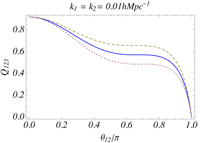
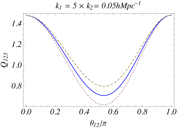
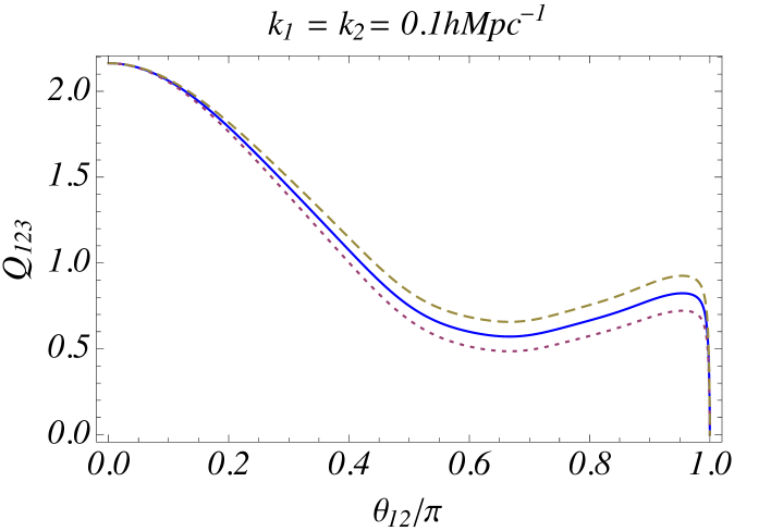
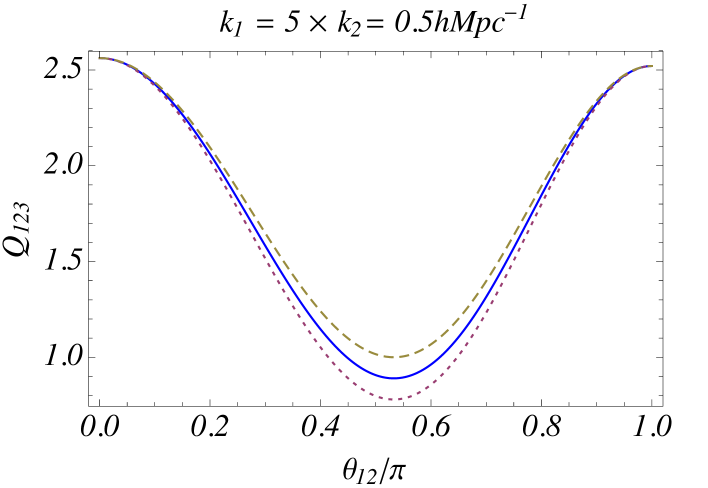
Figure 1: $Q_{123}$ as function of $\theta_{12}$ with fixing, $k_{1}=k_{2}=0.01h{\rm Mpc}^{-1}$ (upper left panel), $k_{1}=k_{2}=0.1h{\rm Mpc}^{-1}$ (lower left panel), $k_{1}=5\times k_{2}=0.05h{\rm Mpc}^{-1}$ (lower right panel), and $k_{1}=5\times k_{2}=0.5h{\rm Mpc}^{-1}$ (lower right panel), respectively. For the linear matter power spectrum $P_{11}(k)$, we adopt the spatially flat universe with the cold dark matter model (CDM) and the cosmological constant $\Lambda$, whose density parameters are $\Omega_{0}=0.3$ and $\Omega_{\Lambda}=0.7$, respectively. Note that the reduced bispectrum depends on time $t$ only through $\lambda(t)$, for which we adopted the different value of $\lambda(t)=1$ (blue solid curve), $\lambda(t)=1.2$ (red dotted curve), and $\lambda(t)=0.8$ (yellow dashed curve), irrespectively of the $\Lambda$CDM model.

$$Q_{123}(t,k_{1},k_{2},\theta_{12}) = {B_{4}(t,k_{1},k_{2},k_{3})\over P_{11}(k_{1})P_{11}(k_{2})+P_{11}(k_{2})P_{11}(k_{3})+P_{11}(k_{3})P_{11}(k_{1})},$$ (82)

at the lowest order of perturbations. Note that the (reduced) bispectrum is described by the kernel (77), which depends only on the parameter $\lambda(t)$, given by (63).

Because ${\bf k}_{1}+{\bf k}_{2}+{\bf k}_{3}=0$ is satisfied, and the reduced bispectrum is a function of only three parameters, which we take $k_{1}=|{\bf k}_{1}|$, $k_{2}=|{\bf k}_{2}|$ and the angle $\theta_{12}$ between ${\bf k}_{1}$ and ${\bf k}_{2}$. Explicit expressions for $\alpha({\bf k}_{i},{\bf k}_{j})$ and $\gamma({\bf k}_{i},{\bf k}_{j})$, where $(i,j)$ denotes any of $(1,2),~{}(2,3)$, or $(3,1)$, are summarized in Appendix B.

Each panel of figure 1 shows a typical behavior of $Q_{123}$ as function of $\theta_{12}$ with fixing $k_{1}$ and $k_{2}$, whose values are described in the caption. In each panel, we adopt the different value of $\lambda(t)=1$ (blue solid curve), $\lambda(t)=1.2$ (red dotted curve), and $\lambda(t)=0.8$ (yellow dashed curve), where we assumed the spatially flat universe with the cold dark matter model (CDM) and the cosmological constant $\Lambda$, whose density parameters are $\Omega_{0}=0.3$ and $\Omega_{\Lambda}=0.7$, for the linear matter power spectrum $P_{11}(k)$. Note that the reduced bispectrum depends on time $t$ only through $\lambda$(t). One can read the following features. First, the overall amplitude of $Q_{123}$ depends on the value of $k_{1}$ and $k_{2}$. However, once the values of $k_{1}$ and $k_{2}$ are fixed, the reduced bispectrum is enhanced for $\lambda<1$, while it is reduced for $\lambda>1$. This feature is explained by the expression of kernel (77) and the fact $\gamma({\bf k}_{i},{\bf k}_{j})\geq 0$.

In the limit $\theta_{12}=0$, we have $\gamma({\bf k}_{1},{\bf k}_{2})=\gamma({\bf k}_{2},{\bf k}_{3})=\gamma({\bf k}_{3},{\bf k}_{1})=0$ (see also appendix B). Then, $Q_{123}$ is independent of $\lambda$ at $\theta_{12}=0$. In the limit $\theta_{12}=\pi$, $Q_{123}$ has the different behavior depending on the conditions $k_{1}=k_{2}$ and $k_{1}\neq k_{2}$. In the case $k_{1}\neq k_{2}$, we have $\gamma({\bf k}_{1},{\bf k}_{2})=\gamma({\bf k}_{2},{\bf k}_{3})=\gamma({\bf k}_{3},{\bf k}_{1})=0$, which is the same as those of the limit $\theta_{12}=0$. In the case $k_{1}=k_{2}$, however, we have $\gamma({\bf k}_{1},{\bf k}_{2})=0,~{}\gamma({\bf k}_{2},{\bf k}_{3})=\gamma({\bf k}_{3},{\bf k}_{1})=1$ , and $k_{3}=0$, i.e, $P_{11}(k_{3})=0$. Then the bispectrum approach zero in this limit, thought the rate of convergence depends on $\lambda(t)$, as is discussed in the next section.

All the influence of the nonlinear interaction of the modified gravity arise only through the parameter $\lambda(t)$, which appears as the term in proportion to $\gamma({\bf k}_{1},{\bf k}_{2})$ in the kernel (77). The bispectrum of the matter density perturbations behaves only in a restricted way, which is a feature of the general second-order scalar-tensor theory equipped with the Vainshtein mechanism.

IV Kinetic gravity braiding model

In this section, we consider a simple example to demonstrate how the modification of gravity influences the behavior of the bispectrum at a quantitative level. We consider the kinetic gravity braiding model investigated in Ref. Deffayet ; kgb , whose action is written as

$$S=\int d^{4}x\sqrt{-g}\left[{M_{\rm pl}^{2}\over 2}R+K-G_{3}\square\phi+{\cal L}_{\rm m}\right],$$ (83)

with the Planck mass $M_{\rm pl}$, which is related with the gravitational constant $G_{N}$ by $8\pi G_{N}=1/M_{\rm pl}^{2}$. Comparing this action (83) with that of the most general second-order scalar-tensor theory, the action of the kinetic gravity braiding model is produced by setting

$$G_{4}={M_{\rm pl}^{2}\over 2},~{}~{}~{}~{}G_{5}=0.$$ (84)

In Ref. kgb , $K$ and $G_{3}$ are chosen as

$$K=-X,~{}~{}~{}~{}G_{3}=M_{\rm pl}\left({r_{c}^{2}\over M_{\rm pl}^{2}}X\right)^{n},$$ (85)

where $n$ and $r_{c}$ are the parameters. In this model, we have

$$L(t)=-{A_{0}{\cal F}_{T}\rho_{\rm m}\over 2(A_{0}{\cal G}_{T}+A_{2}^{2}{\cal F}_{T})},$$ (86)

$$N_{\gamma}(t)={B_{0}A_{2}^{3}{\cal F}_{T}^{3}\rho_{\rm m}^{2}\over 4(A_{0}{\cal G}_{T}^{2}+A_{2}^{2}{\cal F}_{T})^{3}H^{2}}.$$ (87)

Useful expressions of the kinetic gravity braiding model are summarized in Appendix A.

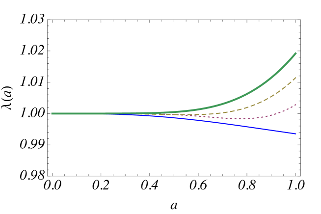
Figure 2: $\lambda(t)$ as function of $a$ for the $\Lambda$CDM model (blue solid curve) and the kinetic gravity braiding model with $n=1$ (red dotted curve), $n=2$ (yellow dashed curve), and $5$ (green thick curve).

When we consider the attractor solution, which satisfies

$$3\dot{\phi}HG_{3X}=1,$$ (88)

the Friedmann equation is written in the form

$$\left({H\over H_{0}}\right)^{2}={\Omega_{0}\over a^{3}}+(1-\Omega_{0})\left({H\over H_{0}}\right)^{-2/(2n-1)},$$ (89)

where $H_{0}$ is the Hubble constant and $\Omega_{0}$ is the density parameter at the present time, and the model parameters must satisfy

$$H_{0}r_{c}=\left({2^{n-1}\over 3n}\right)^{1/2n}\left[{1\over 6(1-\Omega_{0})}\right]^{(2n-1)/4n}.$$ (90)

On the attractor solution, $L(t)$ and $N_{\gamma}(t)$ reduce to

$$L(t)=-{3\over 2}{2n+(3n-1)\Omega_{m}(t)\over 5n-\Omega_{m}(t)}H^{2},$$ (91)

$$N_{\gamma}(t)=-{9\over 4}{(1-\Omega_{m}(t))(2n-\Omega_{m}(t))^{3}\over\Omega_{m}(t)(5n-\Omega_{m}(t))^{3}}H^{2},$$ (92)

where $\Omega_{m}(a)$ is defined by $\Omega_{m}(a)={\Omega_{0}H_{0}^{2}/H(a)^{2}a^{3}}$. Note that the quasi-static approximation on the scales of the large scale structures holds for $n\lower 2.15277pt\hbox{$\;\buildrel<\over{\sim}\;$}10$ (see kgb ).

Figure 2 shows the evolution of $\lambda(t)$ as a function of $a$ for the kinetic gravity braiding model with $n=1,~{}2,~{}5$ and the $\Lambda$CDM model. For $a\ll 1$, we have $\lambda(t)=1$, which is the prediction of the Einstein de Sitter universe. However, the accelerated expansion arises due to a domination of the galileon field as $a$ approaches $1$, then the value of $\lambda(t)$ starts to deviate from $1$. The deviation of $\lambda(t)$ from $1$ is small. The value of $\lambda(t)$ at the present epoch is $0.994$ for the $\Lambda$CDM model with the density parameter $\Omega_{0}=0.3$. The value of $\lambda(t)$ at the present epoch is $1.003$, $1.011$, and $1.019$ for the KBG model with $n=1,~{}2,~{}5$, respectively. Our results guarantee the validity of the approximation setting $\lambda(t)=1$, which is usually adopted in the standard density perturbations theory.

Figure 3 shows the relative deviation of the bispectrum at the present epoch of the KGB model from that of the $\Lambda$CDM model, $Q_{123}(t,k_{1},k_{2},\theta_{12})/$ $Q_{123\Lambda}(t,k_{1},k_{2},\theta_{12})-1$, as a function of $\theta_{12}$, where $Q_{123\Lambda}(t,k_{1},k_{2},\theta_{12})$ is the reduced bispectrum of the $\Lambda$CDM model. The relative deviation from the $\Lambda$CDM model is less than $2$ %. For the case $k_{1}\neq k_{2}$, the deviation between the models does not appear at $\theta_{12}=0,~{}\pi$, which is simply understood by the fact $\gamma({\bf k}_{i},{\bf k}_{j})=0$ there. In the case $k_{1}=k_{2}$ in the limit $\theta_{12}=\pi$, we have $\alpha({\bf k}_{1},{\bf k}_{2})\sim(\pi-\theta_{12})^{2}$, $\alpha({\bf k}_{2},{\bf k}_{3})=\alpha({\bf k}_{3},{\bf k}_{1})=3/4$, $\gamma({\bf k}_{1},{\bf k}_{2})\sim(\pi-\theta_{12})^{2}$, $\gamma({\bf k}_{2},{\bf k}_{3})=\gamma({\bf k}_{3},{\bf k}_{1})=1$, and $P(k_{3})\propto k_{3}^{n_{s}}\propto(\pi-\theta_{12})^{n_{s}}$, where $n_{s}$ is the spectral index. (see appendix B for details.)

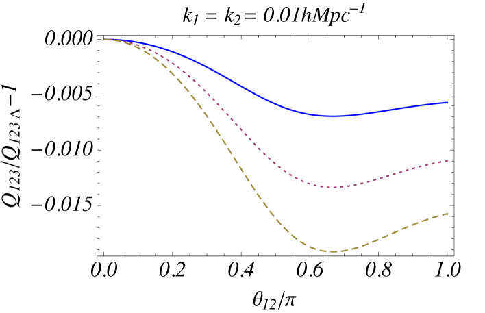
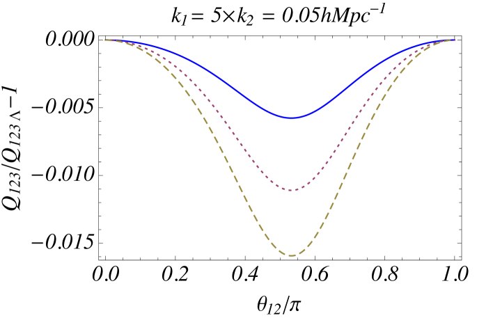
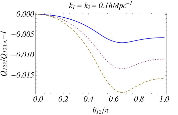
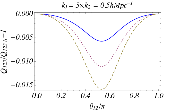
Figure 3: Relative deviation of the reduced bispectrum at the present epoch of the kinetic gravity braiding model with $n=1$ (blue solid curve), $n=2$ (red dotted curve), $n=5$ (yellow dashed curve) from the that of the $\Lambda$CDM model $Q_{123\Lambda}$, as a function of $\theta_{12}$, where $k_{1}$ and $k_{2}$ are fixed, whose values are noted on each panel. Here the density parameter is fixed as $\Omega_{0}=0.3$.

Then, the bispectrum has the asymptotic form

$$B_{4}(t,k_{1},k_{1},\theta_{12})\sim 4\left({3\over 4}-{2\over 7}\lambda(t)\right)P_{11}(k_{3})P_{11}(k_{1})$$ (93)

around the limit $\theta_{12}=\pi$. This leads to the ratio of the reduced bispectrum in this limit,

$${Q_{123}(t,k_{1},k_{1},\theta_{12})\over Q_{123\Lambda}(t,k_{1},k_{1},\theta_{12})}={21-8\lambda(t)\over 21-8\lambda_{\Lambda}(t)},$$ (94)

where $\lambda_{\Lambda}(t)$ is the parameter $\lambda(t)$ of the $\Lambda$CDM model, which explains the behaviors of the left panels of Fig. 3.

The behavior of the reduced bispectrum is almost same when the ratio of $k_{1}/k_{2}$ is the same. This is because the function $\alpha({\bf k}_{i},{\bf k}_{j})$ and $\gamma({\bf k}_{i},{\bf k}_{j})$ depend on only on the ratio $k_{1}/k_{2}$ and $\theta_{12}$ (see also appendix B).

Recently, the bispectrum in the covariant cubic galileon cosmology is investigated in Ref. Emilio . Our kinetic gravity braiding model with $n=1$ is a cubic galileon model, however, there is the difference between our model and the covariant cubic galileon cosmology in Ref. Emilio . The cosmic acceleration in the covariant cubic galileon model is derived by a potential of the scalar field. This causes the differences of the evolution of the background universe and the linear density perturbations.

V Summary and Conclusions

In the present paper, we have investigated the bispectrum of the matter density perturbations induced by the gravitational instability in the most general second-order scalar-tensor theory that may possess the Vainshtein mechanism. We have discussed a general feature of this wide class of modified gravity models in the most general second-order scalar-tensor theory. We have obtained the expression of the bispectrum of the second order of perturbations on the basis of the standard density perturbation theory in an analytic manner. The bispectrum is expressed by the kernel (77), depending only on the parameter $\lambda(t)$, which is determined by the growing and decaying solutions of the linear density perturbations $D_{\pm}(t)$, the Hubble parameter $H(t)$, and the other function $N_{\gamma}(t)$ for the nonlinear interactions. These simple results come from the fact that the basic equations for the gravitational and scalar fields have the same form of the nonlinear mode couplings, which are derived as the leading terms under the quasi-static approximation within the subhorizon scales. Thus, all the effect of the modified gravity in the bispectrum come through the parameter $\lambda(t)$ in the kernel (77), which has the simple structure. This makes the behavior of the bispectrum less complex. As an application of our results, we have exemplified the behavior of the bispectrum in a kinetic gravity braiding model proposed in Ref. kgb . We have investigated the evolution of $\lambda(t)$ in this model, and have demonstrated the deviation of the reduced bispectrum from that of the $\Lambda$CDM model is less than a few %. Higher order solutions of the density perturbations will be obtained in a similar way, which is left as a future problem.

Appendix A Definition of the coefficients

We first summarize the definitions of the coefficients in the field equations in section 2.

$$A_{0} := \frac{\dot{\Theta}}{H^{2}}+\frac{\Theta}{H}+{\cal F}_{T}-2{\cal G}_{T}-2\frac{\dot{\cal G}_{T}}{H}-\frac{{\cal E}+{\cal P}}{2H^{2}},$$ (95)

$$A_{1} := \frac{\dot{\cal G}_{T}}{H}+{\cal G}_{T}-{\cal F}_{T},$$ (96)

$$A_{2} := {\cal G}_{T}-\frac{\Theta}{H},$$ (97)

$$B_{0} := \frac{X}{H}\biggl{\{}\dot{\phi}G_{3X}+3\left(\dot{X}+2HX\right)G_{4XX}+2X\dot{X}G_{4XXX}-3\dot{\phi}G_{4\phi X}+2\dot{\phi}XG_{4\phi XX}$$ (98)

$$+\left(\dot{H}+H^{2}\right)\dot{\phi}G_{5X}+\dot{\phi}\left[2H\dot{X}+\left(\dot{H}+H^{2}\right)X\right]G_{5XX}+H\dot{\phi}X\dot{X}G_{5XXX}$$

$$-2\left(\dot{X}+2HX\right)G_{5\phi X}-\dot{\phi}XG_{5\phi\phi X}-X\left(\dot{X}-2HX\right)G_{5\phi XX}\biggr{\}},$$

$$B_{1} := 2X\left[G_{4X}+\ddot{\phi}\left(G_{5X}+XG_{5XX}\right)-G_{5\phi}+XG_{5\phi X}\right],$$ (99)

$$B_{2} := -2X\left(G_{4X}+2XG_{4XX}+H\dot{\phi}G_{5X}+H\dot{\phi}XG_{5XX}-G_{5\phi}-XG_{5\phi X}\right),$$ (100)

$$B_{3} := H\dot{\phi}XG_{5X},$$ (101)

$$C_{0} := 2X^{2}G_{4XX}+\frac{2X^{2}}{3}\left(2\ddot{\phi}G_{5XX}+\ddot{\phi}XG_{5XXX}-2G_{5\phi X}+XG_{5\phi XX}\right),$$ (102)

$$C_{1} := H\dot{\phi}X\left(G_{5X}+XG_{5XX}\right),$$ (103)

where we also defined

$${\cal F}_{T} := 2\left[G_{4}-X\left(\ddot{\phi}G_{5X}+G_{5\phi}\right)\right],$$ (104)

$${\cal G}_{T} := 2\left[G_{4}-2XG_{4X}-X\left(H\dot{\phi}G_{5X}-G_{5\phi}\right)\right],$$ (105)

$$\Theta := -\dot{\phi}XG_{3X}+2HG_{4}-8HXG_{4X}-8HX^{2}G_{4XX}+\dot{\phi}G_{4\phi}+2X\dot{\phi}G_{4\phi X}$$ (106)

$$-H^{2}\dot{\phi}\left(5XG_{5X}+2X^{2}G_{5XX}\right)+2HX\left(3G_{5\phi}+2XG_{5\phi X}\right),$$

$${\cal E} := 2XK_{X}-K+6X\dot{\phi}HG_{3X}-2XG_{3\phi}-6H^{2}G_{4}+24H^{2}X(G_{4X}+XG_{4XX})$$ (107)

$$-12HX\dot{\phi}G_{4\phi X}-6H\dot{\phi}G_{4\phi}+2H^{3}X\dot{\phi}(5G_{5X}+2XG_{5XX})$$

$$-6H^{2}X(3G_{5\phi}+2XG_{5\phi X}),$$

$${\cal P} := K-2X(G_{3\phi}+\ddot{\phi}G_{3X})+2(3H^{2}+2\dot{H})G_{4}-12H^{2}XG_{4X}-4H\dot{X}G_{4X}$$ (108)

$$-8\dot{H}XG_{4X}-8HX\dot{X}G_{4XX}+2(\ddot{\phi}+2H\dot{\phi})G_{4\phi}+4XG_{4\phi\phi}+4X(\ddot{\phi}-2H\dot{\phi})G_{4\phi X}$$

$$-2X(2H^{3}\dot{\phi}+2H\dot{H}\dot{\phi}+3H^{2}\ddot{\phi})G_{5X}-4H^{2}X^{2}\ddot{\phi}G_{5XX}+4HX(\dot{X}-HX)G_{5\phi X}$$

$$+2\left[2(HX)\dot{}+3H^{2}X\right]G_{5\phi}+4HX\dot{\phi}G_{5\phi\phi}.$$

In the kinetic gravity braiding model considered in section 4, the coefficients are written as follows,

$${\cal F}_{T}=M_{pl}^{2},~{}~{}~{}~{}~{}{\cal G}_{T}=M_{pl}^{2},$$ (109)

$$\Theta=-nM_{pl}\left({r_{c}^{2}\over M_{pl}^{2}}\right)^{n}\dot{\phi}X^{n}+HM_{pl}^{2},$$ (110)

$$\dot{\Theta}=-n(2n+1)M_{pl}\left({r_{c}^{2}\over M_{pl}^{2}}\right)^{n}\ddot{\phi}X^{n}+\dot{H}M_{pl}^{2},$$ (111)

$${\cal E}=-X+6nM_{pl}\left({r_{c}^{2}\over M_{pl}^{2}}\right)^{n}\dot{\phi}HX^{n}-3H^{2}M_{pl}^{2},$$ (112)

$${\cal P}=-X-2nM_{pl}\left({r_{c}^{2}\over M_{pl}^{2}}\right)^{n}\ddot{\phi}X^{n}+(3H^{2}+2\dot{H})M_{pl}^{2},$$ (113)

$$A_{0}={X\over H^{2}}-2nM_{pl}\left({r_{c}^{2}\over M_{pl}^{2}}\right)^{n}\left({2\dot{\phi}\over H}+n{\ddot{\phi}\over H^{2}}\right)X^{n},$$ (114)

$$A_{2}=B_{0}=n{\dot{\phi}\over H}M_{pl}\left({r_{c}^{2}\over M_{pl}^{2}}\right)^{n}X^{n},$$ (115)

$$A_{1}=B_{1}=B_{2}=B_{3}=C_{0}=C_{1}=0.$$ (116)

In the present papwer, we consider the attractor solution satisfying (88), then we have

$$\ddot{\phi}=-{1\over 2n-1}{\dot{\phi}\dot{H}\over H},$$ (117)

$${\dot{H}\over H^{2}}=-{(2n-1)3\Omega_{m}(a)\over 2(2n-\Omega_{m}(a))},$$ (118)

$$A_{0}=-{M_{\rm Pl}^{2}(1-\Omega_{m}(a))\left(2n+(3n-1)\Omega_{m}(a)\right)\over 2n-\Omega_{m}(a)},$$ (119)

$$A_{2}=M_{\rm Pl}^{2}{(1-\Omega_{m}(a))},$$ (120)

$$B_{0}=M_{\rm Pl}^{2}{(1-\Omega_{m}(a))},$$ (121)

where we defined $\Omega_{m}(a)=\rho_{m}(a)/3M_{\rm Pl}^{2}H^{2}$.

Appendix B Explicit expressions of $\alpha$ and $\gamma$

In general, we may write the wave number vector, which satisfies ${\bf k}_{1}+{\bf k}_{2}+{\bf k}_{3}=0$, as follows,

$${\bf k}_{1} = (0,0,k_{1}),$$ (122)

$${\bf k}_{2} = (0,k_{2}\sin\theta_{12},k_{2}\cos\theta_{12}),$$ (123)

$${\bf k}_{3} = (0,-k_{2}\sin\theta_{12},-k_{1}-k_{2}\cos\theta_{12}),$$ (124)

where $\theta_{12}$ is the angle between the vector ${\bf k}_{1}$ and ${\bf k}_{2}$. Then we have

$${{\bf k}_{1}\cdot{\bf k}_{2}\over k_{1}k_{2}}=\cos\theta_{12},$$ (125)

$${{\bf k}_{2}\cdot{\bf k}_{3}\over k_{2}k_{3}}={-k_{2}-k_{1}\cos\theta_{12}\over\sqrt{k_{1}^{2}+k_{2}^{2}+2k_{1}k_{2}\cos\theta_{12}}},$$ (126)

$${{\bf k}_{3}\cdot{\bf k}_{1}\over k_{3}k_{1}}={-k_{1}-k_{2}\cos\theta_{12}\over\sqrt{k_{1}^{2}+k_{2}^{2}+2k_{1}k_{2}\cos\theta_{12}}},$$ (127)

where we used $k_{3}=\sqrt{k_{1}^{2}+k_{2}^{2}+2k_{1}k_{2}\cos\theta_{12}}$. Introducing the constant $c$ by $k_{1}=ck_{2}$, we have

$$k_{3}=k_{1}\sqrt{c^{2}+2c\cos\theta_{12}+1},$$ (128)

$${{\bf k}_{2}\cdot{\bf k}_{3}\over k_{2}k_{3}}=-{c+\cos\theta_{12}\over\sqrt{c^{2}+2c\cos\theta_{12}+1}},$$ (129)

$${{\bf k}_{3}\cdot{\bf k}_{1}\over k_{3}k_{1}}=-{c\cos\theta_{12}+1\over\sqrt{c^{2}+2c\cos\theta_{12}+1}}.$$ (130)

For convenience, we summarize the explicit expressions of $\alpha({\bf k}_{i},{\bf k}_{j})$ and $\gamma({\bf k}_{i},{\bf k}_{j})$. The above relations yield

$$\alpha({\bf k}_{1},{\bf k}_{2})=1+{(c^{2}+1)\cos\theta_{12}\over 2c},$$ (131)

$$\alpha({\bf k}_{2},{\bf k}_{3})=1-{(2c^{2}+2c\cos\theta_{12}+1)(c+\cos\theta_{12})\over 2c(c^{2}+2c\cos\theta_{12}+1)},$$ (132)

$$\alpha({\bf k}_{3},{\bf k}_{1})=1-{(c^{2}+2c\cos\theta_{12}+2)(c\cos\theta_{12}+1)\over 2(c^{2}+2c\cos\theta_{12}+1)},$$ (133)

$$\gamma({\bf k}_{1},{\bf k}_{2})=1-\cos^{2}\theta_{12},$$ (134)

$$\gamma({\bf k}_{2},{\bf k}_{3})={\sin^{2}\theta_{12}\over c^{2}+2c\cos\theta_{12}+1},$$ (135)

$$\gamma({\bf k}_{3},{\bf k}_{1})={c^{2}\sin^{2}\theta_{12}\over c^{2}+2c\cos\theta_{12}+1}.$$ (136)

Thus, $\alpha$ and $\gamma$ depend only on $c$ and $\theta_{12}$, which means that $F_{2}(t,{\bf k}_{i},{\bf k}_{j})$ depends only on $c$ and $\theta_{12}$, excepting $t$. It is trivial that $\alpha({\bf k}_{1},{\bf k}_{2})$ and $\gamma({\bf k}_{1},{\bf k}_{2})$ are invariant under the interchange between ${\bf k}_{1}$ and ${\bf k}_{2}$, or the replacement of $c$ with $1/c$. Note also that $\alpha({\bf k}_{2},{\bf k}_{3})$ and $\gamma({\bf k}_{2},{\bf k}_{3})$ are transformed into $\alpha({\bf k}_{3},{\bf k}_{1})$ and $\gamma({\bf k}_{3},{\bf k}_{1})$, respectively, by the replacement of $c$ with $1/c$.

References

• (1) W. Hu and I. Sawicki, Phys. Rev. D 76 (2007) 064004
• (2) A. A. Starobinsky, JETP Lett. 86 (2007) 157
• (3) S. Tsujikawa, Phys. Rev. D 77 (2008) 023507
• (4) S. Nojiri and S. Odintsov, Phys. Lett. B 657 (2007) 238
• (5) G. R. Dvali, G. Gabadadze and M. Porrati, Phys. Lett. B 485 (2000) 208
• (6) Y-S. Song, I. Sawicki and W. Hu, Phys. Rev. D 75 (2007) 064003
• (7) R. Maartens and E. Majerotto, Phys. Rev. D 74 (2006) 023004
• (8) R. Maartens and K. Koyama, Living Rev. Rel. 13 (2010) 5
• (9) C. de Rham and G. Gabadadze, Phys.Rev. D 82 (2010) 044020
• (10) C. de Rham, G. Gabadadze, and A. J. Tolley, Phys. Rev. Lett. 106 (2011) 231101
• (11) S. F. Hassan and R. A. Rosen, Phys. Rev. Lett. 108 (2012) 041101
• (12) A. R. Gomes, L. Amendola, arXiv1306.3593
• (13) G. W. Horndeski, Int. J. Theor. Phys. 10 (1974) 363
• (14) C. Deffayet, X. Gao, D. A. Steer, and G. Zahariade, Phys. Rev. D 84, (2011) 064039
• (15) T. Kobayashi, M. Yamaguchi, and J. Yokoyama, Prog. Theor. Phys. 126, (2011) 511
• (16) N. Chow and J. Khoury, Phys. Rev. D 80 (2009) 024037
• (17) F. P. Silva and K. Koyama, Phys. Rev. D 80 (2009) 121301
• (18) T. Kobayashi, H. Tashiro and D. Suzuki, Phys. Rev. D 81 (2010) 063513
• (19) T. Kobayashi, Phys. Rev. D 81 (2010) 103533
• (20) A. De Felice and S. Tsujikawa, Phys. Rev. D 84 (2011) 124029
• (21) A. De Felice and S. Tsujikawa, JCAP 07(2010)024
• (22) A. De Felice, S. Mukohyama and S. Tsujikawa, Phys. Rev. D 82 (2010) 023524
• (23) C. Deffayet, G. Esposito-Farese and A. Vikman, Phys. Rev. D 79 (2009) 084003
• (24) R. Gannouji and M. Sami, Phys. Rev. D 82 (2010) 024011
• (25) A. Ali, R. Gannouji and M. Sami, Phys. Rev. D 82 (2010) 103015
• (26) A. De Felice and S. Tsujikawa, Phys. Rev. Lett. 105 (2010) 111301
• (27) S. Nesseris, A. De Felice and S. Tsujikawa, Phys. Rev. D 82 (2010) 124054
• (28) D. F. Mota, M. Sandstad and T. Zlosnik, JHEP 12(2010)051
• (29) A. De Felice, R. Kase, S. Tsujikawa, Phys. Rev. D 83 (2011) 043515
• (30) C. Deffayet, O. Pujolas, I. Sawicki and A. Vikman, JCAP 10(2010)026
• (31) C. Deffayet, S. Deser and G. Esposito-Farese, Phys. Rev. D 80 (2009) 064015
• (32) A. Nicolis, R. Rattazzi and E. Trincherini, Phys. Rev. D 79 (2009) 064036
• (33) C. Burrage and D. Seery, JCAP 08(2010) 011
• (34) G. L. Goon, K. Hinterbichler and M. Trodden, Phys. Rev. D 83 (2011) 085015
• (35) C. de Rham and A. J. Tolley, JCAP 05(2010)015
• (36) R. Kimura, T. Kobayashi, and K. Yamamoto, Phys. Rev. D 85 (2012) 024023
• (37) R. Kase, S. Tsujikawa, JCAP 08(2013)054
• (38) T. Narikawa, T.Kobayashi, D. Yamauchi, R. Saito, Phys. Rev. D 87 (2013) 124006
• (39) Planck Collaboration: P. A. R. Ade et al., arXiv:13035084
• (40) R. Scoccimarro, H. M. Couchman, J. A. Frieman, Astrophy. J. 517, (1999) 531
• (41) T. Nishimichi, et al., Publ. Astron. Soc. Japan 59, (2007) 1049
• (42) F. Bernardeau, S Colombi, E. Gaztanaga, R. Scoccimarro, Phys. Rep. 367 (2002) 1
• (43) N. Bartolo, S. Matarrese and A. Riotto, JCAP 0510 (2005) 010
• (44) N. Bartolo, S. Matarrese and A. Riotto, JCAP 0701 (2007) 019
• (45) K. Koyama, A. Taruya, T. Hiramatsu, Phys. Rev. D 79 (2009) 123512
• (46) A. Barreira, B. Li, W. Hellwing, C. M. Baugh, S. Pascoli, arXiv:1306.3219
• (47) B. Li, A. Barreira, C. M. Baugh, W. A. Hellwing, K. Koyama, arXiv:1308.3491
• (48) M. Wyman, E. Jennings, M. Lima, arXiv:1303.6630
• (49) E. Bellini, N. Bartolo, S. Matarrese, JCAP 1206 (2012) 019
• (50) N. Bartolo, E. Bellini, D. Bertacca and S. Matarrese, JCAP 1303 (2013) 034
• (51) R. Kimura, K. Yamamoto, JCAP 04(2011)025