An Improved Solution for Restricted and Uncertain TRQ

Abstract

CSPTRQ is an interesting problem and its has attracted much attention. The CSPTRQ is a variant of the traditional PTRQ. As objects moving in a constrained-space are common, clearly, it can also find many applications. At the first sight, our problem can be easily tackled by extending existing methods used to answer the PTRQ. Unfortunately, those classical techniques are not well suitable for our problem, due to a set of new challenges. We develop targeted solutions and demonstrate the efficiency and effectiveness of the proposed methods through extensive experiments.

I Introduction

The range query as one of fundamental operations in moving object search systems has attracted a lot of attention in the past decades [43, 12, 40, 36, 31, 20, 24, 19, 18, 14, 3, 9, 26]. A database server usually only stores the discrete location information due to various reasons such as the limited network bandwidth and battery power of the mobile devices [23, 6]. This fact implies that the current specific position of a moving object $o$ is uncertain before obtaining the next (sampled) location information, which can lead to the incorrect answer if we simply take the recorded location (stored in the database) as the current position of $o$. In order to tackle the aforementioned problem, the idea of incorporating uncertainty into the moving object data has been proposed [38]. A widely-used uncertainty model is to use a closed region (known as uncertainty region) together with a probability density function (PDF), which is used to denote the object’s location distribution[38, 6].

From then on, probabilistic range query (PRQ) as a derivative version of the traditional range query was naturally presented, and many outstanding works addressed this problem (see e.g., [8, 27, 23, 33, 4, 28, 35, 6, 42]). In existing results, one of important branches is to address the PRQ over objects moving freely (without predefined routes) in two-dimensional (2D) space (see e.g., [4, 42, 6]). Our work generally falls in the aforementioned branch.

Motivations. A common fact is that users usually are interested in the objects being located in the query range $R$ with higher probabilities. Several classical papers (see e.g., [4, 30, 44]) already considered this fact and studied the probabilistic threshold range query (PTRQ). Existing results are mainly developed for the case of non-constrained 2D space (i.e., no obstacles exist). To our knowledge, the constrained-space probabilistic threshold range query (CSPTRQ) has not been studied yet. Moreover, we realize that more and more intelligent terminals have been configured with touch screens by which one can input the query requirement using the finger or interactive pen [1, 10]. An obvious fact is that a more generic shaped query range should be better for the user experience, and can also improve the flexibility of a system itself. Existing works (see e.g., [27, 28]) already adopted the general polygon as the query range. Those results are mainly developed from the theoretical perspective. Specifically, this work studies the CSPTRQ supporting a generic shaped query range, for moving objects.

The CSPTRQ can be used in a lot of applications, as objects moving in a constrained 2D space are common in the real world. For example, mobile robots are already used to rescue survivors after a disaster such as an earthquake [21]. The location information of robots is collected and stored on the database server. A typical application for dispatching scattered robots to a specific location is retrieving the identities of the robots that are currently located in a given region with no less than a predefined (e.g., $75\%$) probability; here robots usually move freely but can be blocked by various obstacles (e.g., rocks, buildings). As another example, in the information warfare the location information of combat machineries is collected and usually stored on the military database [39, 13]. A typical application for the coordination combat is retrieving the identities of the friendly machineries (e.g., tanks and panzers) that are currently located in a given region with no less than a specific (e.g., $85\%$) probability; here objects such as tanks and panzers usually move freely without predefined routes but can be blocked by various obstacles (e.g., lakes, hills).

Challenges. At the first glance, the CSPTRQ can be easily tackled by directly extending existing methods used to answer the PTRQ. As a matter of fact, there are several new challenges. (i) The CSPTRQ needs to handle a set of obstacles, and so the workload is larger, implying that to achieve a quick response time is more challenging. (ii) With the presence of obstacles, the uncertainty region $u$ is usually a complicated geometry (see Section III-C for more details), rendering that the subsequent computation is more difficult. (iii) In a non-constrained space, $u$ can be easily obtained (almost) without taking the precomputation cost, and thus existing methods usually pre-compute a set of bounds based on the uncertainty region $u$ and the probability density function (PDF). These bounds are used to prune/validate unqualified/qualified objects, and can significantly improve the performance, especially when they are correctly indexed using the R-tree like data structure. In the context of our concern, the precomputation time is rather long (up to the hour level) even if we only pre-compute the uncertainty regions. (See Section III-C for more detailed discussion about bounds and the precomputation.) Imagine if we further pre-compute lots of bounds, the overall precomputation time should be larger. With these challenges (particularly, the third one) in mind, we have to resort to other proposals.

Another method used to answer the constrained-space probabilistic range query (CSPRQ) [37] can be easily extended to tackle our problem. Unfortunately, a simple adaptation of this method is inefficient, due to its weak pruning/validating capability. (See Section III-C for more details about the baseline method.)

Overall, we are confronted with the following troubles: (i) those classical techniques (used to answer the PTRQ) have powerful pruning/validating capabilities, but are not well suitable for the context of our concern, and (ii) the method used to answer the CSPRQ is easily incorporated, but to find a feasible and powerful pruning/validating mechanism is not easy.

Contributions. A casual trifle, shopping in a supermarket, gives us the initial inspiration. The shopper freely chooses his/her wanted commodities and finally obtains them by paying the bill. Clearly, it is a swap: money $\longleftrightarrow$ commodities. This trifle reminds us that swapping can usually obtain the wanted things. With this (concept) in mind, we revisit our problem and develop our first idea — swapping the order of geometric operations, which simplifies the computation and can prune/validate some objects without the need of computing their uncertainty regions. After this, by carefully considering the details, we realize that the result obtained in the previous step possibly is a fake result, which stems from the location unreachability. The natural method to eliminate the fault is inefficient. Instead, our strategy is to take advantage of the location unreachability. This method not only eliminates the possible fault, but also prunes some objects in the early stages. All strategies developed above actually belong to spatial pruning/validating mechanisms.

When we strive to seek the threshold pruning/validating mechanisms, suddenly, we realize an interesting fact — the CSPTRQ can be classified into two forms: explicit and implicit ones (they can have different solutions, performance results, and purposes/applications). The former returns a set of tuples in form of ($o$, $p$) such that $p\geq p_{t}$, where $p$ is the probability of the moving object $o$ being located in the query range $R$, and $0\leq p_{t}\leq 1$ is a given probabilistic threshold. A potential purpose/application is like: listing the objects (e.g., tanks) that are currently located in the region $R$ with no less than the $80\%$ probability in the descending order according to their appearance probabilities; it is similar to the following: listing the universities that are with no less than 80 points in the descending order according to their points, where the points usually be evaluated using a variety of indicators such as the publications in Nature/Science. (Remark: the traditional probabilistic range query (PRQ) usually refers to the explicit form but $p_{t}=0$. Thus, the immediate purposes/applications of the explicit CSPTRQ are the similar as the ones of the traditional PRQ.) In contrast, the latter returns a set of objects, which have probabilities higher than $p_{t}$ to be located in $R$. A potential purpose/application is like: returning the number of objects (e.g., mobile robots) that are currently located in the region $R$ with no less than the $75\%$ probability. (Remark: the traditional probabilistic threshold range query (PTRQ) usually refers to the implicit form. Thus, the immediate purposes/applications of the implicit CSPTRQ are the similar as the ones of the traditional PTRQ.) See Figure 1 for example. We assume there is no obstacles, $R$ is a rectangle, and the location of $o$ follows uniform distribution in $u$ for simplicity. Suppose $p_{t}=0.2$, the answer of explicit query is $\{(o_{2},50\%),$ $(o_{3},50\%),$ $(o_{4},25\%)\}$, while the answer of implicit query is $\{o_{2},o_{3},o_{4}\}$.

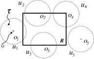
Figure 1: Example of explicit and implicit queries, where $l_{r}$ denotes the recorded location, $\tau$ denotes the distance threshold, and $u_{i}$ denotes the uncertainty region of object $o_{i}$ ($i\in[1,2,\cdots,5]$)

The second main idea is inspired by the evolutionary algorithms [16]. A typical characteristic of evolutionary algorithms is the repeated application of a set of predefined operators; and each iteration can be generally looked as a refinement of the previous result. This reminds us to compute the appearance probability $p$ in a multi-step manner, and thus objects that are obviously unqualified can be pruned in the early steps. This idea is especially effective when the locations of objects do not follow uniform distribution in their uncertainty regions. The multi-step strategy yields a set of threshold pruning/validating rules, which are employed by the explicit query. As the implicit query does not need to return the appearance probabilities of qualified objects, an enhanced multi-step strategy is naturally developed, which includes an adaptive pruning/validating mechanism and a two-way test mechanism. Furthermore, we further optimize our solutions based on a new insight — different candidate moving objects may share the same candidate restricted areas. In summary, our contributions are as follows:

We propose the CSPTRQ, and show that (i) it can be used in many applications; (ii) the classical methods used to answer the traditional PTRQ are not well suitable for the context of our concern; and (iii) a simple adaptation of the method used to answer the CSPRQ is inefficient.

We realize the CSPTRQ can be classified into two forms: explicit and implicit ones. We formally formulate them, and offer insights into their properties.

We develop techniques to answer the explicit query, and then extend them to answer the implicit query. Our solutions are simple but without loss of efficiency.

We give the detailed theoretical analysis for our algorithms. While we focus on the CSPTRQ in this paper, (part of) our techniques can be immediately extended to other types of probabilistic threshold queries.

We experimentally evaluate our algorithms using both real and synthetic data sets. The experimental results demonstrate the efficiency and effectiveness of the proposed algorithms. From the experimental results, we can further perceive the difference between explicit and implicit queries. This interesting finding is valuable especially for the topics of other types of probabilistic threshold queries.

Paper organization. We review the related work in Section II. We formally formulate our problem and present a baseline method in Section III. The proposed methods for answering the explicit and implicit CSPTRQs are addressed in Section IV and V, respectively. We further optimize our solution based on a new insight in Section VI. We evaluate the performance of our proposed methods through extensive experiments in Section VII. Finally, we conclude this paper with several interesting research topics in Section VIII.

II Related work

Range query over moving objects. Most of the representative works on range query over moving objects have been mentioned in Section I. A common aspect of those works is not to capture the location uncertainty. In other words, they assume the current location of any object $o$ is equal to the recorded location (stored on the database server). In contrast, we assume the current location of $o$ is uncertain.

Uncertainty models. We also mentioned many outstanding works on PRQ over uncertain moving objects in Section I. One of important branches assumed that objects move freely (without predefined routes) in 2D space. In this branch, there are several typical uncertainty models like, the free moving uncertainty (FMU) model [6, 38], the moving object spatial temporal (MOST) model [27], the uncertain moving object (UMO) model [42], the 3D cylindrical (3DC) model [35, 23], and the necklace uncertainty (NU) model [34, 17]. Another important branch assumed that objects move on predefined routes [6] or road networks [45]. They usually adopt the line segment uncertainty (LSU) model [8, 6] to capture the location uncertainty. These models have different assumptions and purposes (e.g., 3DC and NU models are suitable for querying the trajectories of moving objects), but have their own advantages (note: it is a difficult task to say which one is the best. Please refer to [37] as a summary on the differences of these models and their assumptions). The model used in [37] roughly follows the FMU model, but it is different from the FUM model, as it introduces the concept of restricted areas (i.e., obstacles). Here we dub it the extensive free moving uncertainty (EFMU) model for clearness.

Though our work also uses the EFMU model, there are at least two differences: (i) our work investigates CSPTRQs (including explicit and implicit ones) rather than the CSPRQ, and (ii) our work employs a more generic shaped query range.

Probabilistic threshold range query. According to the theme of this paper, we classify PTRQs into two subcategories: PTRQs for moving objects and the ones for other uncertain data (note: the terms “PRQ” and “PTRQ” are somewhat abused in the literature, we take those papers, which explicitly discussed the probabilistic threshold, as the related work of the PTRQ).

Many excellent works addressed the PTRQ for moving objects. For example, Chung et al. [8] addressed the PTRQ for objects moving in one-dimensional (1D) space. In contrast, we focus on the objects moving in 2D space. Zhang et al. [42] studied the PTRQ over objects moving in 2D space. They proposed the UMO model, in which they assumed both the distribution of velocity and the one of location are available at the update time. In contrast, we do not need to know the velocity (as well as its distribution), instead we assume the specific location of any object $o$ is available at the update time. Moreover, the used model in this paper is the EFMU model, which considers the existence of restricted areas. Zheng et al. [45] studied the PTRQ for objects moving on the road networks. They proposed the UTH model that is developed for querying the trajectories of moving objects. In contrast, this paper is not interested in querying the trajectories, and it focuses on the objects moving in the constrained 2D space where no predefined route is given.

There are many classical papers that studied the PTRQ for other uncertain data. For example, Cheng et al. [7] addressed the PTRQ over 1D uncertain data (e.g. sensor data), they presented a clever idea, using a tighter bound (compared to the MBR of the uncertainty interval), called x-bound, to reduce the search cost. Later, Tao et al. [32] extended this idea to multi-dimensional uncertain data. They proposed a classical technique, probabilistic constrained region (PCR), which consists of a set of precomputed bounds, called p-bounds. This classical technique is not well suitable for the context of our concern, Section I has shown the reasons (more detailed discussion will be given in Section III-C). Chen et al. [4] studied the PTRQ for such a scenario where the location of query issuer is uncertain (a.k.a, location based PTRQ); several smart ideas such as the query expansion were developed. They assumed the query range $R$ and uncertainty region $u$ are rectangles, and focused on the non-constrained space, and thus employed the p-bounds technique. In contrast, both $R$ and $u$ used in our work are more complex, and we focus on the constrained space, where the p-bounds technique has some limitations (again, Section I has shown the reasons). Moreover, our work does not belong to the location based PTRQ.

Other probabilistic threshold queries. There are also many representative works that addressed other probabilistic threshold queries (PTQs); those works are clearly different from ours. For instance, Zhang et al. studied the location based probabilistic threshold range aggregated query [44]. Hua et al. [15] addressed the probabilistic threshold ranking query on uncertain data. The probabilistic threshold KNN query over uncertain data was investigated by Cheng et al. [5]. Yuan et al. [41] discussed the probabilistic threshold shortest path query over uncertain graphs. The general PTQ for arbitrary SQL queries that involve selections, projections, and joins was studied by Qi et al. [25].

III Problem definition

III-A Problem settings and notations

Let $R$ be the query range. Let $r$ denote the restricted area, and ${\mathscr{R}}$ be a set of disjoint restricted areas. Let $\mathbb{T}$ be a territory such that $\bigcup_{r\in\mathscr{R}}{r}\subset{\mathbb{T}}$. Let $o$ denote the moving object, and ${\mathscr{O}}$ be a set of moving objects. Let $l_{r}$ be the latest recorded location (stored on the database server) of $o$, and $l_{t}$ be the location of $o$ at an arbitrary instant of time $t$. We assume that $l_{t}\notin\bigcup_{r\in{\mathscr{R}}}{r}$ and $l_{t}\in{\mathbb{T}}-\bigcup_{r\in{\mathscr{R}}}{r}$. Let $\tau$ be the distance threshold of $o$. We assume any object $o$ reports its new location to the server once $dist(l_{t_{n}},l_{r})\geq$ $\tau$, where $l_{t_{n}}$ denotes its current specific location, $dist(\cdot)$ denotes the Euclidean distance. Finally, for any two different objects $o$ and $o^{\prime}$, we assume they cannot be located in the same location at the same instant of time $t$, i.e., $l_{t}\neq l_{t}^{\prime}$.

We model both the query range and restricted areas as the arbitrary shaped polygons. We capture the location uncertainty using two components [6, 38].

Definition III.1 (Uncertainty region).

The uncertainty region of a moving object $o$ at a given time $t$, denoted by $u^{t}$, is a closed region where $o$ can always be found.

Definition III.2 (Uncertainty probability density function).

The uncertainty probability density function of $o$ at time $t$, denoted by $f^{t}(x,y)$, is a probability density function (PDF) of $o$’s location at a given time $t$; its value is 0 if $l_{t}$ $\notin$ ${u}^{t}$.

The PDF has the property that $\int_{{u}^{t}}f^{t}(x,y)dxdy=1$. In addition, under the distance based update policy (a.k.a., dead-reckoning policy [38, 6]), for any two different time $t_{1}$ and $t_{2}$ ($t_{1},t_{2}\in$ ($t_{r}$,$t_{n}$]), the following conditions always hold: $u^{t_{1}}=u^{t_{2}}$ and $f^{t_{1}}(x,y)=f^{t_{2}}(x,y)$, where $t_{r}$ refers to the latest reporting time, $t_{n}$ refers to the current time. Hence, unless stated otherwise, we use $u$ and $f(x,y)$ to denote the uncertainty region and PDF of $o$, respectively. (Remark: if the time based update policy is assumed to be adopted, such a topic is more interesting and also more challenging, since the uncertainty region $u$ is to be a continuously changing geometry over time. See, e.g., [37] for a clue about the relation between the location update policy and the uncertainty region $u$.) With the presence of restricted areas (i.e., obstacles), the uncertainty region $u$ under the distance based update policy can be formalized as follows.

$$u=o.\odot-\bigcup_{r\in{\mathscr{R}}}r$$ (1)

where $o.\odot$ denotes a circle with the centre $l_{r}$ and radius $\tau$. We remark that, in the rest of this paper, we abuse the notation ‘$|\cdot|$’, but its meaning should be clear from the context. In addition, unless stated otherwise, a notation or symbol with a subscript ‘b’ usually refers to its corresponding minimum bounding rectangle (MBR). For instance, $R_{b}$ refers to the MBR of $R$. For convenience, Table I summarizes the notations used frequently in the rest of this paper.

Notations	Meanings
$\mathscr{R}^{*}$	the set of candidate restricted areas
$\mathscr{O}^{*}$	the set of candidate moving objects
$R_{b}$	the minimum bounding rectangle of the query range $R$
$\tau$	distance threshold
$l_{r}$	recorded location of a moving object $o$
$o.\odot$	circle with the centre $l_{r}$ and radius $\tau$
$\mathscr{I}_{r}$	index of restricted areas
$\mathscr{I}_{o}$	index of moving objects
$p_{t}$	probabilistic threshold
$u_{o}$	outer ring of uncertainty region $u$
$u_{h}^{i}$	the $i$th hole in uncertainty region $u$
$\mathscr{H}$	the set of holes in uncertainty region $u$
$s$	intersection result between $R$ and $u$
$|s|$	the number of subdivisions of $s$
$s[i]$	the $i$th subdivision of $s$
$s[i]_{o}$	outer ring of $s[i]$
$\mathscr{H}^{*}$	the set of all holes in $s$
$s_{h}^{j}$	the $j$th hole among all the $|\mathscr{H}^{*}|$ holes of $s$
$\gamma$	reference value

TABLE I: Notations and their descriptions

III-B Problem statement

Let $p_{t}$ be the probabilistic threshold, we have

Definition III.3.

Given a set $\mathscr{R}$ of restricted areas, a set $\mathscr{O}$ of moving objects in a territory $\mathbb{T}$, and a query range $R$, an explicit constrained-space probabilistic threshold range query (ECSPTRQ) returns a set of tuples in form of ($o$, $p$) such that $p\geq p_{t}$, where $p$ is the probability of $o$ being located in $R$, and is computed as

$$p=\int_{u\cap R}f(x,y)dxdy$$ (2)

We note that $f(x,y)$=$\frac{1}{\alpha(u)}$ when the location of $o$ follows uniform distribution in its uncertainty region $u$, where $\alpha(\cdot)$ denotes the area of this geometric entity. In this case, we have

$$p=\frac{\alpha(u\cap R)}{\alpha(u)}$$ (3)

Definition III.4.

Given a set $\mathscr{R}$ of restricted areas, a set $\mathscr{O}$ of moving objects in a territory $\mathbb{T}$, and a query range $R$, an implicit constrained-space probabilistic threshold range query (ICSPTRQ) returns all the objects $o$ such that $p\geq p_{t}$, where $p$ is the probability of $o$ being located in $R$, and is computed according to Equation (2).

We remark that though the differences of two queries above are minor at the first glance, we will present different solutions respectively in Section IV and V, and show their different performance results in Section VII. Sometimes, we also use terms the explicit query and the implicit query to denote the above two queries in the rest of this paper. For ease of understanding the proposed methods, we next introduce a baseline method.

III-C Baseline method

The baseline method is a simple adaptation of the method in [37]. To save space, we only present an overall framework of the baseline method.

Preprocessing stage. Here a twin-index is adopted (e.g., a pair of R-trees or its variant): one is used to manage the set $\mathscr{R}$ of restricted areas; another is used to manage the set $\mathscr{O}$ of moving objects. To index restricted areas is simple, since we model them as arbitrary polygons. Naturally, we can easily find the MBR of any restricted area $r$ ($\in\mathscr{R}$). In order to manage the set $\mathscr{O}$ of moving objects, we here index them based on their recorded locations $l_{r}$ and distance thresholds $\tau$. Specifically, for each object $o$, its MBR is a square centering at $l_{r}$ with $2\tau\times 2\tau$ size. For clearness, let ${\mathscr{I}}_{o}$ and ${\mathscr{I}}_{r}$ be the index of moving objects and the one of restricted areas, respectively.

Query processing stage. We first give two definitions before discussing the details.

Definition III.5 (Candidate moving object).

Given a moving object $o$ and the query range ${R}$, $o$ is a candidate moving object such that $R_{b}\cap o.\odot_{b}$$\neq$$\emptyset$.

Definition III.6 (Candidate restricted area).

Given a moving object $o$ and a restricted area $r$, $r$ is a candidate restricted area such that $r_{b}\cap o.\odot_{b}$$\neq$$\emptyset$.

Let ${\mathscr{R}^{*}}$ denote the set of candidate restricted areas, and ${\mathscr{O}^{*}}$ denote the set of candidate moving objects. There are several main steps for answering the implicit (or explicit) query. First, we search ${\mathscr{O}^{*}}$ on $\mathscr{I}_{o}$ using $R_{b}$ as the input (here most of unrelated objects are to be pruned). Second, for each object $o\in\mathscr{O}^{*}$, we search $\mathscr{R}^{*}$ on $\mathscr{I}_{r}$ using $o.\odot_{b}$ as the input (here most of unrelated restricted areas are to be pruned). We compute $o$’s uncertainty region $u$, and then compute “$u\cap R$”. After this, we compute $p$ using Equation (2). We put $o$ (or ($o,p$)) into the result if $p\geq p_{t}$. Otherwise, we discard it and process the next object. After all candidate moving objects are handled, we finally return the result, in which all qualified objects are included.

Update stage. When an object $o$ reports its new location to the server, we update the database record, i.e., $l_{r}$. At the same time, we update the index of moving objects, i.e., ${\mathscr{I}}_{o}$.

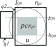
(a)

(b)

(c)

(d)

Figure 2: Illustration of of p-bounds and the precomutaion. (a) The case of no restricted areas. (b) The case of existing restricted areas. (c) The uncertainty region. (d) The precomputaion time when $|\mathscr{R}|=|\mathscr{O}|=50k$. $\zeta$ denotes the number of edges in each restricted area $r$ (note: it may be somewhat difficult to understand this figure, and the readers can revisit it after reading Section VII).

Discussion. The readers may be curious why the baseline method does not employ existing threshold pruning/validating mechanisms such as p-bounds in [32, 4, 30, 44]. Briefly speaking, a p-bound of the uncertainty region $u$ (of the object $o$) is a function of $p$, where $p\in[0,0.5]$. A probabilistically constrained region (PCR) with the parameter $p$, denoted by $o.pcr(p)$, consists of four p-bounds, namely $l(p)$, $r(p)$, $t(p)$ and $b(p)$, see the four dashed lines in Figure 2(a). The line $l(p)$ divides the uncertainty region $u$ (i.e., the circle) into two parts (on the left and right of $l(p)$ respectively), and the appearance probability of $o$ on the left part equals $p$. (Other three lines have similar meanings.) The grey region illustrates $o.pcr(p)$. Assume the parameter $p$ in Figure 2(a) is 0.2; moreover, assume the probabilistic threshold $p_{t}=0.8$, and if $q1$ is the query range, then $o$ is an unqualified object, and thus to be pruned. In contrast, if $q2$ is the query range, then $o$ is a qualified object, and thus to be validated. The example above illustrates the rationale of the classical p-bounds technique. In a non-constrained space (i.e., no obstacles exist), all the uncertainty regions can be easily obtained (almost) without taking the precomputation cost, and thus pre-computing a set of p-bounds is feasible. However, in the context of our concern, the precomputation time is rather long (up to the hour level) even if we only pre-compute the uncertainty regions. Figure 2(d) reports the time of pre-computing a set of uncertainty regions. Imagine if we further pre-compute lots of p-bounds, then the overall precomputation time should be larger. This is the main reason why the p-bounds technique is not well suitable for our problem. Other minor (non-fatal) reasons have already been mentioned in Section I. For example, the closed region with many holes shown in Figure 2(c) illustrates the uncertainty region $u$, which is derived from Figure 2(b) based on Equation (1). Clearly, to obtain $o.pcr(p)$ in Figure 2(c) is more difficult than the case of no restricted areas (e.g., see Figure 2(a)).

To this step, it seems no better solution except the baseline method. A casual trifle, shopping in a supermarket, gives us the initial inspiration (recall Section I). In the next section, we show the details of our ideas, and then present the algorithm to answer the explicit query.

IV Explicit CSPTRQ

IV-A Spatial pruning/validating rules

For each object $o\in\mathscr{O}^{*}$, once we obtain the set $\mathscr{R}^{*}$ of candidate restricted areas, the baseline method is to directly compute its uncertainty region $u$, and then to compute the intersection result between $R$ and $u$. Let $s$ be the intersection result between $R$ and $u$, it can be formalized as follows.

$$s=u\cap R=(o.\odot-\bigcup_{r\in\mathscr{R}^{*}}r)\cap R$$ (4)

Our method is to swap the order of geometric operations. The rationale behind it is surprisingly simple. Specifically, we first compute “$o.\odot\cap R$”, and then use the result of “$o.\odot\cap R$” to subtract $\bigcup_{r\in\mathscr{R}^{*}}r$. It is formalized as follows.

$$s=(o.\odot\cap R)-\bigcup_{r\in\mathscr{R}^{*}}r$$ (5)

There are two significant benefits by swapping the order of geometric operations.

(1) We can prune some objects, without the need of computing their uncertainty regions. Assume “q1” shown in Figure 3(a) is the query range $R$. Clearly, $o$ is a candidate moving object since $o.\odot_{b}$ intersects with $R_{b}$. Here $o$ can be safely pruned without the need of computing its uncertainty region $u$, since “$R\cap o.\odot=\emptyset$”. Similarly, assume that “q2” is $R$. Here “$R\cap o.\odot\neq\emptyset$” (see Figure 3(a)), but $(o.\odot\cap R)-\bigcup_{r\in\mathscr{R}^{*}}r=\emptyset$ (see Figure 3(b)). Hence $o$ can also be pruned safely without the need of computing $u$.

(2) We no longer need to consider each $r\in\mathscr{R}^{*}$, which simplifies the computation of $s$. For example, regarding to “q2”, only the right most candidate restricted area is relevant with the computation of $s$. Similarly, regarding to “q3” shown in Figure 3(b), only two candidate restricted areas are relevant with the computation of $s$.

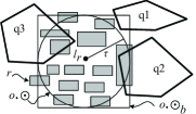
(a)

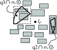
(b)

Figure 3: Example of swapping the order of gemetric operations

Hence, by swapping the order of geometric operations, we can easily develop the following pruning/validating rules.

Lemma IV.1.

Given the query range $R$ and an object $o\in\mathscr{O}^{*}$, we have

If $R\cap o.\odot=\emptyset$, then $o$ can be pruned safely.

If $R\cap o.\odot=o.\odot$, then $o$ can be validated safely.

Proof. The proof is immediate by analytic geometry. $\square$

Let ${\mathscr{R}}^{\prime}$ be a set of restricted areas such that the MBR of each $r\in{\mathscr{R}}^{\prime}$ has non-empty intersection set with the MBR of $o.\odot\cap R$, we have an immediate corollary below.

Corollary IV.1.

Given the query range $R$ and an object $o\in\mathscr{O}^{*}$, $o$ can be pruned safely if $(o.\odot\cap R)-\bigcup_{r\in\mathscr{R}^{\prime}}r=\emptyset$. $\square$

Discussion. We remark that the swapping operation itself is very easy, as it does not rely on any complicated technique. Furthermore, after we swap the order of geometric operations, to develop the pruning/validating rules is also not difficult. We highlight it because it is surprisingly simple but clearly efficient.

Now, for any object $o\in\mathscr{O}^{*}$, if it has not been pruned (or validated) by Lemma IV.1 or Corollary IV.1, whether or not we can directly compute its appearance probability $p$ using Equation (2)? At the first sight, it seems to be sure. However, we should note that the intersection result $s$ obtained by Equation (5) is possibly a fake result. We next share our insights and explain the details.

IV-A1 Why is it possibly a fake result?

The fake result stems from the location unreachability. To explain it, we need some basic concepts.

Given $o.\odot$ and a set $\mathscr{R}^{*}$ of candidate restricted areas, we say a restricted area $r\in\mathscr{R}^{*}$ can subdivide $o.\odot$, if and only if the result of “$o.\odot-r$” consists of multiple disjoint closed regions. We term each of those closed regions as a subdivision. Let $\mathscr{D}$ denote the set of subdivisions, we say a subdivision $d\in\mathscr{D}$ is an effective subdivision such that $l_{r}\in d$, where $l_{r}$ is the (latest) recorded location of $o$ (recall Section III-A).

Theorem IV.1.

Assume that a restricted area $r\in\mathscr{R}^{*}$ subdivides $o.\odot$, and $\mathscr{D}$ is the set of subdivisions, if a subdivision $d\in\mathscr{D}$ is not the effective subdivision, then any point $p^{\prime}\in d$ is unreachable.

Proof. It is easy to know that the object $o$ is located in $o.\odot$, as we adopt the distance based update policy, recall Section III-A. We prove $p^{\prime}\in d$ is unreachable by contraction. Assume that $o$ can reach the point $p^{\prime}$, implying that there exists at least a path from $l_{r}$ to $p^{\prime}$ such that it does not directly pass through any restricted area and also the boundary of $o.\odot$. However, by the condition “$d$ is not the effective subdivision”, implying that $l_{r}$ and $p^{\prime}$ are located respectively in two disjoint closed regions. Based on analytic geometry, it is clear that no such a path exists. This completes the proof. $\square$

Theorem IV.1 gives us the insight into the location unreachability. See Figure 4(a) for example, here the subdivision above $r_{1}$ and the one below $r_{2}$ are unreachable. Hence, $o$’s real uncertainty region, $u$, is the subdivision below $r_{1}$ and above $r_{2}$. With this (concept) in mind, we next use a more targeted example to show why $s$ obtained by Equation (5) possibly is a fake result. The shadow region shown in Figure 5(a) or 5(b) illustrates $s$ obtained by Equation (5), which is not equal to $\emptyset$. Here $o$ cannot be pruned/validated based on Lemma IV.1 and Corollary IV.1. The closed region with many holes shown in Figure 5(b) illustrates $u$. For simplicity, assume that the location of $o$ follows uniform distribution in $u$. In this example, if we simply use the area of the shadow region to divide the area of $u$, we will get that $p$ is a positive number rather than 0. Clearly, it is a false answer, since $u$ and $s$ are disjoint, see Figure 5(b).

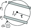
(a)

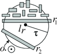
(b)

Figure 4: Illustration of the location unreachability

IV-A2 Natural solution

To eliminate the fault produced by the above problem, the natural solution is to compute $u$, and then to check if $u$ intersects with $s$. If they are disjoint, then $p=0$ and $o$ should be pruned. This approach can indeed be used to eliminate the fault but it is inefficient. We next review two approaches [37] that are used to compute $u$, and then show the underlying reason.

Given a closed region $c$, we let $v^{-}$, $v^{+}$, $h^{-}$, $h^{+}$ denote the four (left, right, bottom, top) bounding lines of $c$, respectively. The span of $c$ is $\mathop{\mathrm{argmax}}\{dist(v^{-},v^{+}),$ $dist(h^{-},h^{+})\}$, where $dist(\cdot)$ denotes the Euclidean distance.

Heuristic 1.

Given $o.\odot$, and two different candidate restricted areas, the candidate restricted area with the larger span is more likely to subdivide $o.\odot$ into multiple subdivisions.

To compute $u$, there are two approaches. The first one is using $o.\odot$ to subtract each restricted area $r\in\mathscr{R}^{*}$ one by one, and finally it chooses the subdivision containing the point $l_{r}$ as the uncertainty region $u$ (see, e.g., Figure 4(a)). For ease of describing the second approach, we let $d^{e}$ denote the effective subdivision (recall Section IV-A1), and slightly abuse the notation $d^{e}$.

The second one incorporates Heuristic 1, and can be generally described as follows. First, it sorts the set $\mathscr{R}^{*}$ of candidate restricted areas according to their spans in the descending order (implying that the restricted area $r\in\mathscr{R}^{*}$ with the larger span is to be handled firstly); and then it uses $o.\odot$ to subtract each $r\in\mathscr{R}^{*}$ one by one; particularly, when multiple subdivisions appear, it immediately chooses the effective subdivision $d^{e}$, and then uses $d^{e}$ to subtract the next $r\in\mathscr{R}^{*}$, and so on; it finally gets $u$ after all the restricted areas $r\in\mathscr{R}^{*}$ are handled. See Figure 4(b), $r_{1}$ is to be handled at first. The subdivision below $r_{1}$ is taken as $d^{e}$. Then, it uses $d^{e}$ to subtract $r_{2}$. Here, the subdivision below $r_{1}$ and above $r_{2}$ is taken as $d^{e}$. After this, the rest of restricted areas can be quickly pruned and thus do not need to execute (costly) geometric subtraction operations, improving the first approach.

Why is it inefficient? Consider the example in Figure 5(a) again, we can easily see that, if we want to get the uncertainty region $u$, both of the approaches mentioned above need to execute subtraction operations many times. This justifies the natural solution mentioned in the beginning of Section IV-A2 is inefficient. Our strategy is to fight poison with poison. In other words, we take advantage of the location uncertainty. This method is pretty simple, but clearly efficient. The challenge is to find the point of penetration, namely, when, where, and how to take advantage of the location unreachability.

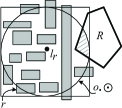
(a)

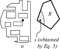
(b)

Figure 5: Illustration of the fake result

IV-A3 Take advantage of the location unreachability

Based on the definition of subdivision, the nature of location unreachability, and Equation (5), we can build the following theorem.

Theorem IV.2.

Given $o.\odot$ and $\mathscr{R}^{*}$, $s$ (obtained by Equation (5)) is always a correct result such that for any $r\in\mathscr{R}^{*}$, $|o.\odot-r|=1$, where $|\cdot|$ denotes the number of subdivisions.

Theorem 1 implies that the presence of multiple subdivisions (i.e., $|o.\odot-r|>1$) is an important sign of the fault to be happened. Hence, if we correctly and timely handle this special case, the possible fault could be eliminated efficiently. With this (concept) in mind, a more efficient solution comes into being. Specifically, we manage to compute its uncertainty region $u$; in the process of computing $u$, once multiple subdivisions appear, we also choose the effective subdivision $d^{e}$, but we do not directly use $d^{e}$ to subtract the next candidate restricted area. Instead, we here check the geometric relation between $d^{e}$ and $s$ (obtained by Equation (5)).

Lemma IV.2.

If $s\cap d^{e}=\emptyset$, then $o$ can be pruned safely.

Proof. The proof is not difficult but (somewhat) long, we move it to Appendix A. $\square$

We note that $s$ obtained by Equation (5) possibly consists of multiple subdivisions. From Lemma IV.2, we have an immediate corollary below.

Corollary IV.2.

Given $o.\odot$ and $R$, we assume $s$ (obtained by Equation (5)) consists of multiple subdivisions, say $s[1]$, $s[2]$, $\cdots$, $s{[|s|]}$, where $|s|$ is the total number of subdivisions in $s$. Without loss of generality, assume that $r\in\mathscr{R}^{*}$ can subdivide $o.\odot$ into multiple subdivisions, and $d^{e}$ is the effective subdivision. We have that, any subdivision $s[i]$ ($i\in[1,\cdots,|s|]$) can be pruned safely if $s[i]\cap d^{e}=\emptyset$. $\square$

While this method is pretty simple, we can easily see that it gains two benefits: it not only eliminates the possible fault produced by Equation (5), but also prunes some objects in the early stages, without the need of obtaining the final results of their uncertainty regions. See, e.g., Figure 5(a), $o$ can be pruned after executing (only) one subtraction operation.

Discussion. All mechanisms discussed before belong to spatial pruning/validating mechanisms. For any object $o$ that has not been pruned/validated by the above mechanisms, the natural method is to compute its appearance probability $p$ using Equation (2) or (3), and then to see if $p\geq p_{t}$, where $p_{t}$ is the so-called probabilistic threshold. In the next subsection, we present a more efficient method, which is initially inspired by evolutionary algorithms (recall Section I). We remark that $s$ (discussed in the rest of this paper) refers to the correct result since we already eliminated the possible fault.

IV-B Threshold pruning/validating rules

Our method computes $p$ in a multi-step rather than one-time way. We call it the multi-step mechanism. Briefly speaking, we first obtain a coarse-version result (CVR), which is possibly far away from the accurate value of $p$. We then make a comparison between the CVR and $p_{t}$, and check if $o$ can be pruned based on the current information. If otherwise, we refine the CVR by the further computation.

IV-B1 Uniform distribution PDF

To apply the multi-step mechanism to the case of uniform distribution PDF, we need to find appropriate carriers (or things) to which we can apply the multi-step mechanism.

Suppose that there is a closed region with many holes. Its exact area clearly equals that the area of the closed region subtracts the areas of all holes. In contrast, if we compute the area of the closed region, but do not subtract the areas of holes, we shall get the most coarse result. Furthermore, we can easily see that this coarse result can be gradually refined by subtracting the rest of holes one by one. Hence, the holes here are taken as the carriers. Based on this intuition, it is not difficult to develop the followings.

For ease of understanding the details, we first should note that the uncertainty region $u$ is a single subdivision (possibly) with holes; and $s$ may be multiple subdivisions (i.e., $|s|>1$) and each subdivision (possibly) has holes. Given a closed region $c$ with a hole $h$, we say the boundary of $c$ is the outer ring of $c$, and say the boundary of $h$ is the inner ring of $c$. We also use $\alpha(\cdot)$ to denote the area of a geometry.

Let $u_{o}$ be the outer ring of uncertainty region $u$, $u_{h}^{i}$ be the $i$th hole in $u$, and $\mathscr{H}$ be the set of holes in $u$, where $|\mathscr{H}|\geq 0$. We have

$$\alpha(u)=\alpha(u_{o})-\sum_{i=0}^{|\mathscr{H}|}\alpha(u_{h}^{i})$$ (6)

Similarly, let $s[i]$ be the $i$th subdivision of $s$, $s[i]_{o}$ be the outer ring of $s[i]$, $s[i]_{h}^{j}$ be the $j$th hole in $s[i]$, and $|s[i]_{h}|$ be the number of holes in $s[i]$. We have

$$\alpha(s)=\sum_{i=1}^{|s|}\alpha(s[i])=\sum_{i=1}^{|s|}{\left(\alpha(s[i]_{o})-\sum_{j=0}^{|s[i]_{h}|}\alpha(s[i]_{h}^{j})\right)}$$ (7)

For ease of presentation, we let $\mathscr{H}^{*}$ denote the set of (all) holes in $s$ (note: $|\mathscr{H}^{*}|=\sum_{i=0}^{|s|}|s[i]_{h}|$), and renumber these holes. Specifically, we let $s_{h}^{j}$ denote the $j$th hole among all the $|\mathscr{H}^{*}|$ holes. Therefore, Equation (7) can be rewritten as follows.

$$\alpha(s)=\sum_{i=1}^{|s|}{\alpha(s[i]_{o})}-\sum_{j=0}^{|\mathscr{H}^{*}|}\alpha(s_{h}^{j})$$ (8)

The natural solution (one-time way) is to compute $\alpha(u)$ and $\alpha(s)$ based on Equation (6) and (8), respectively, and then to check if $\frac{\alpha(s)}{\alpha(u)}\geq p_{t}$.

In the proposed method, we also compute $\alpha(u)$. We however, do not directly compute $\alpha(s)$. Specifically, we initially compute $\sum_{i=1}^{|s|}\alpha(s[i]_{o})$. Then, we compute the first CVR, denoted by $p^{0}$, as follows.

$$p^{0}=\frac{\sum_{i=1}^{|s|}\alpha(s[i]_{o})}{\alpha(u)}$$ (9)

Lemma IV.3.

Given $p^{0}$ and the probability threshold $p_{t}$, $o$ can be pruned safely if $p^{0}$$<p_{t}$.

Proof. We only need to show that the appearance probability $p$ is less than $p_{t}$. Let $\epsilon$ denote an arbitrary non-negative number. We have

$$p^{0}=\frac{\sum_{i=1}^{|s|}\alpha(s[i]_{o})}{\alpha(u)}\geq\frac{(\sum_{i=1}^{|s|}\alpha(s[i]_{o})-\epsilon}{\alpha(u)}$$ (10)

In addition, since $p=\frac{\alpha(s)}{\alpha(u)}$, by Equation (8), we have

$$p=\frac{\sum_{i=1}^{|s|}{\alpha(s[i]_{o})}-\sum_{j=0}^{|\mathscr{H}^{*}|}\alpha(s_{h}^{j})}{\alpha(u)}$$ (11)

Clearly, “$\sum_{j=0}^{|\mathscr{H}^{*}|}\alpha(s_{h}^{j})$” in Equation (11) is a non-negative number. By Formula (10) and Equation (11), we have $p\leq p^{0}$. Combining the condition “$p^{0}<p_{t}$”, hence $p<p_{t}$. $\square$

If the object $o$ cannot be pruned based on Lemma IV.3, and there exist holes in $s$, we further compute the second CVR, and so on. Let $p^{k-1}$ be the $k$th CVR, where $1<k\leq|\mathscr{H}^{*}|+1$. We have

$$p^{k-1}=\frac{\sum_{i=1}^{|s|}\alpha(s[i]_{o})-\sum_{j=0}^{k-1}\alpha(s_{h}^{j})}{\alpha(u)}$$ (12)

We should note that $p^{k-1}=p$ when $k=|\mathscr{H}^{*}|+1$. In other words, the final CVR is equal to the appearance probability $p$. Furthermore, $\sum_{j=0}^{k-1}\alpha(s_{h}^{j})\leq\sum_{j=0}^{|\mathscr{H}^{*}|}\alpha(s_{h}^{j})$, since $1<k\leq|\mathscr{H}^{*}|+1$. Hence, from Lemma IV.3, we have an immediate corollary below.

Corollary IV.3.

Given the $k$th CVR $p^{k-1}$ and the probability threshold $p_{t}$, $o$ can be pruned safely if $p^{k-1}<p_{t}$. $\square$

Discussion. We have shown how to apply the multi-step mechanism to the case of uniform distribution PDF, and developed new pruning rules. The small challenge is to find appropriate carriers to which we can apply the multi-step mechanism. To apply this mechanism to the case of non-uniform distribution PDF, there is also a small challenge, which however, is different from the previous, as we can easily find appropriate carriers by the similar observation. To explain this small challenge, we need some preliminaries. In the next subsection, we first introduce the preliminaries, then clarify this small challenge, and finally give the details of our method .

IV-B2 Non-uniform distribution PDF

Regarding to the non-uniform distribution PDF, a classical numerical integration method is the Monte Carlo method [4, 30, 6]. Let $N_{1}$ denote a pre-set value, where $N_{1}$ is an integer. The natural solution is to randomly generate $N_{1}$ points in the uncertainty region $u$. For each generated point $p^{\prime}$, it computes the value $f(x_{i},y_{i})$ based on its PDF, where $(x_{i},y_{i})$ are the coordinates of the point $p^{\prime}$, and then to check if $p^{\prime}\in s$. Without loss of generality, assume that $N_{2}$ points (among $N_{1}$ points) are to be located in $s$. Then

$$p=\frac{\sum_{i=1}^{N_{2}}f(x_{i},y_{i})}{\sum_{i=1}^{N_{1}}f(x_{i},y_{i})}$$ (13)

Finally, it checks if $p$$\geq p_{t}$. If so, it puts the tuple $(o,p)$ into the result. Otherwise, $o$ is to be pruned.

We should note that the Monte Carlo method is a non-deterministic algorithm. Thus we usually use a large sample as the input, in order to assure the accuracy of computation. Here the number of generated points is the size of sample. In general, the larger $N_{1}$ is, the workload error is more close to 0. Without loss of generality, assume that the allowable workload error is $\delta$, we can get the specific value of $N_{1}$ by the off-line test.

To this step, we can easily realize that the generated points can be taken as carriers to which we can apply the multi-step mechanism. In other words, the following steps are easily brought to mind: we initially generate a small number of points, and thus get a coarse result; then, we refine the previous coarse result by gradually adding points. A small challenge is to construct the pruning rules. In other words, assume that we get a coarse result, how to decide whether or not $o$ can be pruned based on the current coarse result and the probabilistic threshold $p_{t}$.

To alleviate the small challenge above, we take advantage of the workload error. Henceforth, we can easily determine whether or not $o$ can be pruned based on three parameters: the current coarse result, its corresponding workload error, and the probabilistic threshold $p_{t}$. We remark that the workload error can also be estimated by the off-line test, when we use a small number of points. (In our experiments, we use the maximum workload error. For example, assume there are 100 approximate values, say $x_{a}^{i}$, where $i\in[1,100]$, and assume the exact value is $x_{e}$. Then, the maximum workload error for this single value is $\mathop{\mathrm{argmax}}\{|x_{e}-x_{a}^{i}|\}$. By the extensive off-line test, an overall maximum workload error thus can be estimated. Again, the Monte Carlo method is a non-deterministic algorithm, thus the extensive off-line test is needed, in order to assure the accuracy of computation.) Once we get rid of this small challenge, it is not difficult to develop the followings.

Specifically, in the proposed method, we do not directly generate $N_{1}$ points; instead we initially generate $\lfloor\frac{N_{1}}{\theta}\rfloor$ points in $u$, where $\theta$ is an integer (e.g., 10). Let $N_{2}^{0}$ be the number of points being located in $s$, where $N_{2}^{0}\leq\lfloor\frac{N_{1}}{\theta}\rfloor$. Then, we get the first CVR $p^{0}$ as follows.

$$p^{0}=\frac{\sum_{i=1}^{N_{2}^{0}}f(x_{i},y_{i})}{\sum_{i=1}^{\lfloor\frac{N_{1}}{\theta}\rfloor}f(x_{i},y_{i})}$$ (14)

Let $\delta^{0}$ be the workload error when we use $\lfloor\frac{N_{1}}{\theta}\rfloor$ points as the input. We have

Lemma IV.4.

If $p^{0}$ $+\delta^{0}<$$p_{t}$, then $o$ can be pruned safely.

Proof. Let $V_{\infty}$ be the value obtained by Equation (13) when we set $N_{1}\rightarrow+\infty$ (note: in this case the workload error can be taken as 0). It is clearly that $p^{0}-\delta^{0}\leq V_{\infty}\leq p^{0}+\delta^{0}$. Incorporating the condition “$p^{0}$ $+\delta^{0}<$$p_{t}$”, hence $V_{\infty}<p_{t}$. This completes the proof. $\square$

If $o$ cannot be pruned based on Lemma IV.4, we refine the first CVR by adding points. For the $k$th coarse-version, we denote by $\lfloor\frac{k\cdot N_{1}}{\theta}\rfloor$, $\delta^{k-1}$, and $N_{2}^{k-1}$ the number of generated points, the workload error and the number of points being located in $s$, respectively. Then, the $k$th CVR $p^{k-1}$ ($1<k\leq\theta$) can be derived as follows.

$$p^{k-1}=\frac{\sum_{i=1}^{N_{2}^{k-1}}f(x_{i},y_{i})}{\sum_{i=1}^{\lfloor\frac{k\cdot N_{1}}{\theta}\rfloor}f(x_{i},y_{i})}$$ (15)

Furthermore, since each coarse-version corresponds to a workload error, from Lemma IV.4, we have an immediate corollary below.

Corollary IV.4.

Given the probability threshold $p_{t}$, the $k$th CVR $p^{k-1}$ and its corresponding workload error $\delta^{k-1}$. If $p^{k-1}$ $+\delta^{k-1}<$$p_{t}$, then $o$ can be pruned safely. $\square$

Up to now, we have shown all our pruning/validating rules (including spatial and threshold ones), we next pull them together to answer the explicit query.

IV-C Query processing for explicit CSPTRQ

IV-C1 Algorithm

Let $\Re$ be the query result. Recall that ${\mathscr{R}}^{\prime}$ be a set of restricted areas such that the MBR of each $r\in{\mathscr{R}}^{\prime}$ has non-empty intersection set with the MBR of $o.\odot\cap R$ (cf. Section IV-A). Furthermore, we use $u[temp]$ to denote the intermediate result of the uncertainty region $u$ (since we manage to compute the uncertainty region $u$, and hope some objects can be pruned in the early stages, recall Section IV-A3); similarly, we use $p[temp]$ to denote the intermediate result of $p$ (since we adopt multi-step way to compute the appearance probability $p$, recall Section IV-B).

We first search the set $\mathscr{O}^{*}$ of candidate moving objects on the index ${\mathscr{I}}_{o}$ using $R_{b}$ as the input. We then process each object $o\in\mathscr{O}^{*}$ based on Algorithm 1 below. Note that in the following algorithm, the clause “Discard $o$” denotes that the object $o$ is to be pruned, and we shift to process the next object, without the need of executing the remaining lines.

 

Algorithm 1 Explicit CSPTRQ

 

(1)   if $o.\odot\subseteq R$

(2)      Set $p\leftarrow 1$, and let $\Re\leftarrow\Re\cup$$(o,p)$ // $o$ be validated, Lemma IV.1

(3)   else if $o.\odot\cap$$R=\emptyset$

(4)      Discard $o$ // $o$ be pruned, Lemma IV.1

(5)   else // $o.\odot\cap$ $R\neq\emptyset$

(6)      Obtain ${\mathscr{R}}^{\prime}$ by searching on ${\mathscr{I}}_{r}$, and set $s\leftarrow$ ($o.\odot\cap R$)$-\cup_{r\in\mathscr{R}^{\prime}}r$

(7)      if $s=\emptyset$

(8)          Discard $o$ // $o$ be pruned, Corollary IV.1

(9)      else // $s\neq\emptyset$

(10)        Obtain $\mathscr{R}^{*}$ by searching on ${\mathscr{I}}_{r}$, set $u[temp]\leftarrow o.\odot$, and

          sort all the restricted area $r$$\in\mathscr{R}^{*}$ according to their spans

(11)        for each $r$ $\in\mathscr{R}^{*}$

(12)           Let $u[temp]\leftarrow u[temp]-r$

(13)           if $|u[temp]|>1$ // multiple subdivisions appear

(14)              $u[temp]\leftarrow$Choose the effective subdivision

(15)           if $u[temp]$ and $s$ are disjoint

(16)              Discard $o$ // $o$ be pruned, Lemma IV.2

(17)           for each $s[i]$ // $s[i]$ is a subdivision of $s$

(18)              if $u[temp]\cap s[i]=\emptyset$

(19)                 Remove $s[i]$ from $s$ // Corollary IV.2

(20)        Set $u\leftarrow u[temp]$

(21)        $p[temp]\leftarrow$ Compute the first CVR // Eq. 9 (or 14)

(22)        if $p[temp]<$$p_{t}$ (or $p[temp]+\delta^{0}<p_{t}$)

(23)           Discard $o$ // $o$ be pruned, Lemma IV.3 (or IV.4)

(24)        else

(25)           while $p[temp]$ is not the final CVR

(26)              $p[temp]\leftarrow$Compute the next CVR //Eq. 12 (or 15)

(27)              if $p[temp]<p_{t}$ (or $p[temp]+\delta^{k-1}<p_{t}$)

(28)                 Discard $o$ // $o$ be pruned, Corollary IV.3 (or IV.4)

(29)           Set $p\leftarrow p[temp]$, and let $\Re\leftarrow\Re\cup(o,p)$ // $o$ cannot be pruned by all the rules

 

We remark that we overlook the cost such as adding a tuple $(o,p)$ into $\Re$, comparing the geometric relation between two entities, etc., as these costs are trivial. Moreover, the span is a real number, hence the overhead to sort $|\mathscr{R}^{*}|$ candidate restricted areas is pretty small and can (almost) be overlooked compared to the overhead to execute $O(|\mathscr{R}^{*}|)$ times geometric subtraction operations. In the sequel, we show how to extend techniques proposed in this section to answer the implicit query.

V Implicit CSPTRQ

We first introduce the enhanced multi-step computation, and then integrate the techniques proposed in Section IV-A to answer the implicit query. The enhance multi-step computation is easily brought to mind, as we have discussed the multi-step computation in the previous section, and we can easily see that the implicit query does not need to return the appearance probabilities of qualified objects, implying that some threshold validating rules can be developed. Note that the performance differences between the explicit and implicit queries stem mainly from this step.

V-A Enhanced multi-step computation

The enhance multi-step strategy includes (i) an adaptive pruning/validating mechanism, which is used for the uniform distribution case, and (ii) a two-way test mechanism, which is used for the non-uniform distribution case. Regarding to the two-way test mechanism, there is no much surprise. Regarding to the first mechanism, its central idea is to cleverly choose appropriate rule (or method) according to the specific case. A small challenge can be generally described as follows: given two methods and a specific case, how to determine which method is more suitable for this specific case? In the sequel, we discuss more details. (Remark: most of notations discussed later actually have already been defined in previous sections, if any question, please refer to Table I and/or Section IV-B.)

V-A1 Adaptive pruning/validating mechanism

Recall the tactic discussed in Section IV-B1. For the first coarse-version result (CVR), it is to compute $\alpha(u)$ and $\sum_{i=1}^{|s|}\alpha(s[i]_{o})$ at first, and then to compute the first CVR $p^{0}$ based on Equation (9). Since the implicit query does not need to explicitly return the probabilities of the qualified objects, clearly, it is also feasible that we first compute $\alpha(s)$ and $\alpha(u_{o})$, and then compute the first CVR $p^{0}$ as follows.

$$p^{0}=\frac{\alpha(s)}{\alpha(u_{o})}$$ (16)

Lemma V.1.

Given the probability threshold $p_{t}$ and the first CVR $p^{0}$ (obtained by Equation (16)), we have that if the first CVR $p^{0}$$>p_{t}$, then $o$ can be validated safely.

Proof. We only need to show $p$$>p_{t}$. The proof is the similar as the one of Lemma IV.3. $\square$

If $o$ cannot be validated based on Lemma V.1, and the number of holes in $u$ is not equal to 0 (i.e., $|\mathscr{H}|\neq 0$), we further compute the second CVR, and so on. Then, the $k$th CVR $p^{k-1}$ ($1<k\leq|\mathscr{H}|+1$) can be derived as follows.

$$p^{k-1}=\frac{\alpha(s)}{\alpha(u_{o})-\sum_{i=0}^{k-1}\alpha(u_{h}^{i})}$$ (17)

Note that $p^{k-1}$ equals the appearance probability $p$ when $k=|\mathscr{H}|+1$. Furthermore, $\sum_{i=0}^{k-1}\alpha(u_{h}^{i})$ $\leq$ $\sum_{i=0}^{|\mathscr{H}|}\alpha(u_{h}^{i})$, since $1<k\leq|\mathscr{H}|+1$. Hence, from Lemma V.1, we have an immediate corollary below.

Corollary V.1.

Given the probability threshold $p_{t}$ and the $k$th CVR $p^{k-1}$ (obtained by Equation (17)), $o$ can be validated safely, if $p^{k-1}>p_{t}$. $\square$

Hence, we can easily see that, if an object $o$ cannot be pruned/validated based on the spatial information, then there are two methods to handle it.

Method 1: We compute the CVRs according to Equation (9) or (12), and then check if $o$ can be pruned based on Lemma IV.3 or Corollary IV.3.

Method 2: We compute the CVRs according to Equation (16) or (17), and then check if $o$ can be validated based on Lemma V.1 or Corollary V.1.

The naive solution is always to use one of the two methods to handle those candidate moving objects that cannot be pruned/validated by the spatial information. Instead, we adopt an adaptive pruning/validating mechanism. In brief, if $o$ is more likely to be pruned, we use the “Method 1”; in contrast, if $o$ is more likely to be validated, we use the “Method 2”. Note that, there is a question “given an object $o$, how to know it is more likely to be pruned (or validated)?”

Specifically, we compute a reference value, which is used to estimate the trend of $o$ (being more likely to be pruned/validated). Let $\gamma$ denote the reference value, which is computed as follows.

$$\gamma=\frac{\sum_{i=1}^{|s|}\alpha(s[i]_{o})}{\alpha(u_{o})}$$ (18)

Heuristic 2.

Given $\gamma$ and $p_{t}$, if $\gamma<p_{t}$, then $o$ is more likely to be pruned. Otherwise, $o$ is more likely to be validated.

Algorithm 2 below shows the pseudo codes of the adaptive pruning/validating mechanism. Lines 2-10 focus on pruning objects, and Lines 12-20 focus on validating objects. (Note that the meanings of the notations used in this algorithm are the same as the ones in Algorithm 1.)

 

Algorithm 2 Adaptive pruning/validating mechanism

 

(1)    $\gamma\leftarrow$Compute the reference value // Equation (18)

(2)    if $\gamma<p_{t}$

(3)        $p[temp]\leftarrow$Compute the first CVR // Equation (9)

(4)        if $p[temp]<$$p_{t}$

(5)            Discard $o$ // $o$ be pruned, Lemma IV.3

(6)        else

(7)            while $p[temp]$ is not the final CVR

(8)                $p[temp]\leftarrow$Compute the next CVR // Equation (12)

(9)                if $p[temp]<p_{t}$

(10)                  Discard $o$ // $o$ be pruned, Corollary IV.3

(11)          Let $\Re\leftarrow\Re\cup o$ // $o$ is a qualified object

(12)  else // $\gamma\geq p_{t}$

(13)      $p[temp]\leftarrow$Compute the first CVR // Equation (16)

(14)      if $p[temp]\geq p_{t}$

(15)          Let $\Re\leftarrow\Re\cup o$ // $o$ be validated, Lemma V.1

(16)      else

(17)          while $p[temp]$ is not the final CVR

(18)              $p[temp]\leftarrow$Compute the next CVR // Equation (17)

(19)              if $p[temp]\geq p_{t}$

(20)                  Let $\Re\leftarrow\Re\cup o$ // $o$ be validated, Corollary V.1

(21)          Discard $o$ // $o$ is an unqualified object

 

V-A2 Two-way test mechanism

The two-way test mechanism is a simple extension of the method in Section IV-B. For the sake of completeness, we present it below.

Regarding to the first CVR, we can also compute it according to Equation (14). Then, we have

Lemma V.2.

Given the probability threshold $p_{t}$, the first CVR $p^{0}$ and its corresponding workload error $\delta^{0}$, we have

If “$p^{0}$ $+\delta^{0}<p_{t}$”, then $o$ can be pruned safely.

If “$p^{0}$ $-\delta^{0}\geq p_{t}$”, then $o$ can be validated safely.

Proof. It is immediate by extending the proof of Lemma IV.4. $\square$

If $o$ can be neither pruned nor validated based on Lemma V.2, we further compute the second CVR, and so on. For the $k$th CVR, we can also compute it according to Equation (15). From Lemma V.2, we have an immediate corollary below.

Corollary V.2.

Given the probability threshold $p_{t}$, the $k$th CVR $p^{k-1}$ and its corresponding workload error $\delta^{k-1}$, we have

If “$p^{k-1}$ $+\delta^{k-1}<p_{t}$”, then $o$ can be pruned safely.

If “$p^{k-1}-$$\delta^{k-1}\geq p_{t}$”, then $o$ can be validated safely. $\square$

The pseudo codes of the two-way test mechanism are shown in Algorithm 3. We remark that in the two-way test mechanism, if $o$ cannot (still) be pruned/validated by the final CVR, we take the object $o$ as a qualified object, since the final CVR equals $p$, and $p\in[p-\delta,p+\delta]$, where $\delta$ is the allowable workload error.

V-B Query processing for implicit CSPTRQ

Algorithm. The spatial pruning/validating mechanisms proposed in Section IV-A can be seamlessly incorporated for answering the implicit query, implying that the algorithm for the implicit query is the similar as the one for the explicit query. Specifically, we need to replace Line 2 and Lines 21-29 in Algorithm 1 with new pseudo codes. Clearly, Line 2 should be replaced by “${\Re\leftarrow\Re\cup o}$”, and Lines 21-29 should be replaced by the pseudo codes of the enhanced multi-step computation, i.e., Algorithms 2 and 3.

I/O and query cost. The I/O cost is the same as the one of Algorithm 1. The query cost can be estimated using the similar method presented in Section IV-C. Specifically, the $i$ in Equation (LABEL:equation:query_cost) should be replaced with a more small value, since the enhanced multi-step mechanism not only prunes but also validates objects.

 

Algorithm 3 Two-way test mechanism

 

(1)    $p[temp]\leftarrow$ compute the first CVR // Equation (14)

(2)    if $p[temp]+\delta^{0}<p_{t}$ $\parallel$ $p[temp]-\delta^{0}\geq p_{t}$

(3)        if $p[temp]+\delta^{0}<p_{t}$

(4)            Discard $o$ // $o$ be pruned, Lemma V.2

(5)        else // $p[temp]-\delta^{0}\geq p_{t}$

(6)            $\Re\leftarrow\Re\cup o$ // $o$ be validated, Lemma V.2

(7)    else

(8)        while $p[temp]$ is not the final CVR

(9)            $p[temp]\leftarrow$Compute the next CVR // Equation (15)

(10)          if $p[temp]+\delta^{k-1}<p_{t}$ $\parallel$ $p[temp]-\delta^{k-1}\geq p_{t}$

(11)              if $p[temp]+\delta^{k-1}<p_{t}$

(12)                  Discard $o$ // $o$ be pruned, Corollary V.2

(13)              else // $p[temp]-\delta^{k-1}\geq p_{t}$

(14)                  $\Re\leftarrow\Re\cup o$ // $o$ be validated, Corollary V.2

(15)      $\Re\leftarrow\Re\cup o$

 

VI Further optimization

In previous sections, for each candidate moving object $o\in\mathscr{O}^{*}$ we retrieve the set $\mathscr{R}^{\prime}$ of restricted areas from the database and then compute $s$, if $o$ cannot be pruned/validated by Lemma IV.1. Particularly, we further retrieve the set $\mathscr{R}^{*}$ of restricted areas from the database and then compute $u$, if $o$ cannot still be pruned by Corollary IV.1 (c.f., Algorithm 1). Note that there is an overlap between $\mathscr{R}^{\prime}$ and $\mathscr{R}^{*}$ (as $\mathscr{R}^{\prime}\subseteq\mathscr{R}^{*}$). This implies that in this case we retrieve two times for the $|\mathscr{R}^{\prime}|$ restricted areas, which incurs the extra I/O cost. With the similar observation we can also realize that for different candidate moving objects, their candidate restricted areas may have an overlap. This implies that previous methods retrieve multiple times for those “overlapped” restricted areas, which also incurs the extra I/O cost.

To overcome the above limitations, we develop a novel strategy. The rationale behind this strategy is to track restricted areas that have been retrieved, avoiding to retrieve redundant data from the database. Generally speaking, for each restricted area that has been retrieved from the database, we use the $<$key,value$>$ pair to store the ID and geometric data of restricted area in memory. For brevity, we denote by $D_{m}$ the data structure used to manage the set of $<$key,value$>$ pairs. Furthermore, we build another R-tree, which is used to index restricted areas that have been retrieved. Here the leaf node does not store the detailed geometric data of restricted area, instead it only stores the ID and MBR of restricted area. We denote by $\mathscr{I}_{r}^{\prime}$ this R-tree for clearness. With the help of $D_{m}$ and $\mathscr{I}_{r}^{\prime}$, we can easily track the restricted areas that have been retrieved. Specifically, we do as follows:

If we need to obtain $\mathscr{R}^{\prime}$ (or $\mathscr{R}^{*}$), we do not directly search on $\mathscr{I}_{r}$ and fetch restricted area data from the database. Instead, we first search on $\mathscr{I}_{r}^{\prime}$, getting a set, say $S_{1}$, of IDs of restricted areas (note: these restricted area data can be obtained by accessing $D_{m}$ which is stored in memory); we then search on $\mathscr{I}_{r}$, getting another set, say $S_{2}$, of IDs of restricted areas. Let $S_{3}$ be the set of IDs of restricted areas such that $S_{3}=S_{2}-S_{1}$. We here only need to fetch restricted area data (from the database) whose IDs are in $S_{3}$. The $|S_{3}|$ restricted areas fetched from the database and the $|S_{1}|$ ones obtained from $D_{m}$ constitute $\mathscr{R}^{\prime}$ (or $\mathscr{R}^{*}$).

If restricted areas are fetched from the database, we immediately index these restricted areas using $\mathscr{I}_{r}^{\prime}$, and add corresponding $<$key,value$>$ pairs into $D_{m}$. That is to say, we update $\mathscr{I}_{r}^{\prime}$ and $D_{m}$ immediately once we fetched restricted area data from the database.

With the above concepts in mind, we can easily develop the improved algorithm for the explicit query. First, we search the set $\mathscr{O}^{*}$ of candidate moving objects on the index ${\mathscr{I}}_{o}$ using $R_{b}$ as the input. We then initialize $D_{m}$ and $\mathscr{I}_{r}^{\prime}$. Next, we process each object $o\in\mathscr{O}^{*}$. The steps of processing each object $o$ are the similar as the ones in Algorithm 1, except that we need to make minor modifications on Lines 6 and 10 (here we use the strategy proposed in this section). Note that, the improved algorithm for implicit query is available by similar modifications. The pseudo codes of these two improved algorithms are immediate, and thus are omitted for saving space. In the next section, we test the effectiveness and efficiency of the proposed algorithms, using extensive experiments under various experimental settings.

VII Experimental evaluation

VII-A Experimental setup

Our experiments are based on both real and synthetic data sets, and the size of 2D space is fixed to 10000$\times$10000. Two real data sets called CA and LB, are deployed. The data sets are the similar as the ones in [6, 11, 30]. The CA contains 104770 2D points, the LB contains 53145 2D rectangles. We let the CA denote the (latest) recorded locations of moving objects, and the LB denote the restricted areas. (Remark: this paper is not interested in querying the trajectories, and thus does not use the trajectory data sets.) All data sets are normalized in order to fit the 10000$\times$10000 2D space. Synthetic data sets also consist of two types of data. We generate a set of polygons to denote the restricted areas, and place them in this space uniformly. We generate a set of points to denote the (latest) recorded locations of moving objects, and let them randomly distributed in this space (note: there is a constraint that these points cannot be located in the interior of any restricted area). Moreover, we randomly generate different distant thresholds (between 20 and 50) for different moving objects. For brevity, we use the CL and RU to denote the real (California points together with Long Beach rectangles) and synthetic (Random distributed points together with Uniform distributed polygons) data sets, respectively.

Parameter	Description	Value
$N$	number of moving objects	[$10k,20k,30k,40k,\textbf{50k}$]
$M$	number of restricted areas	[$10k,20k,30k,40k,\textbf{50k}$]
$\zeta$	number of edges of each $r$	[$\textbf{4},8,16,32,64$]
$\psi$	number of edges of $R$	[$\textbf{4},8,16,32,64$]
$\epsilon$	size of $R$	[$100,200,300,400,\textbf{500}$]
$p_{t}$	probabilistic threshold	[$0.1,0.3,0.5,\textbf{0.7},0.9$]
$\eta$	shape of $R$	[ Sq,Ta,Dm,Tz,Cc ]
$N_{1}$	number of pre-set points	[ 700 ]
$\theta$	number of versions	[ 7 ]

TABLE II: Parameters Used in Our Experiments

The performance metrics include the preprocessing time, update time, I/O time and query time. Specifically, the query time is the sum of I/O and CPU time. The update time is the sum of the time for updating the database record (i.e., $l_{r}$) and the one for updating the index ${\mathscr{I}}_{o}$, when an object reports its new location to the database server (note: we here do not consider the network transfer time). In order to investigate the update time, we randomly update 100 location records, and run 10 times for each test, and then compute the average value for estimating a single location update. To estimate the average I/O and query time of a single query, we randomly generate 50 query ranges, and run 10 times for each query range, and then compute the average value. Also, we run 10 times and compute the average value for estimating the preprocessing time.

Shape	Value
Ta	[$(x,y),(x+L,y),(x+L/2,y+L)$]
Tz	[$(x,y),(x+L,y),(x+2L/3,y+L),(x+L/3,y+L)$]
Dm	[$(x+L/2,y),(x+2L/3,y+L/3),(x+L,y+L/2),(x+2L/3,y+2L/3),(x+L/2,y+L),(x+L/3,y+2L/3),(x,y+L/2),(x+L/3,y+L/3)$]
Cc	[$(x+L/3,y),(x+2L/3,y),(x+2L/3,y+L/3),(x+L,y+L/3),(x+L,y+2L/3),(x+2L/3,y+2L/3),(x+2L/3,y+L),(x+L/3,y+L),(x+L/3,y+2L/3),(x,y+2L/3),(x,y+L/3),(x+L/3,y+L/3)$]

TABLE III: Use Cases of $\eta$

Our experiments are conducted on a computer with 2.16GHz dual core CPU and 1.86GB of memory. The page size is fixed to 4K. The maximum number of children nodes in the R-tree ${\mathscr{I}}_{o}$ (${\mathscr{I}}_{r}$) is fixed to 50. The (latest) recorded locations of moving objects and the restricted areas are stored using the MYSQL Spatial Extensions. (Henceforth, we call them location records and restricted area records, respectively.) Other parameters are listed in Table II, in which the numbers in bold denote the default settings. $N$, $M$ and $\zeta$ are the settings of synthetic data sets. The default setting of each restricted area $r$ is a rectangle with $40\times 10$ size. Sq, Ta, Dm, Tz and Cc denote square, triangle, diamond, trapezoid and crosscriss, respectively. The specific settings of these geometries are listed in Table III. These geometries are all bounded by the $500\times 500$ rectangular box (i.e., MBR). $L$ in Table III is 500, and $(x,y)$ are the coordinates of left-bottom point of its MBR, which are generated randomly. We use two types of PDFs: uniform distribution and distorted Gaussian. We use the UD and DG to denote them, respectively. In our experiments, the standard deviation is set to $\frac{\tau}{5}$ (note: $\tau$ is the distance threshold), and the mean $u_{x}$ and $u_{y}$ are set to the coordinates of the recorded location $l_{r}$. Following the guidance of [37], we choose 700 as the number of pre-set points. In addition, we use 7 coarse versions for the multi-step computation, corresponding workload errors (WEs) are listed in Table IV, these data are obtained by the off-line test. All workload errors refer to the absolute workload errors. More specifically, $CV_{7}$ is the average (absolute) workload error, other versions are the maximum (absolute) workload errors. We remark that although $\theta=7$ is not mandatory, a too small value weakens the efficiency of the multi-step mechanism, and a too large value incurs not only over-tedious tests, but also negligible pruning/validating power between two consecutive versions.

Property	$CV_{1}$	$CV_{2}$	$CV_{3}$	$CV_{4}$	$CV_{5}$	$CV_{6}$	$CV_{7}$
$\lfloor\frac{k\cdot N_{1}}{\theta}\rfloor$	100	200	300	400	500	600	700
WE	0.3607	0.2499	0.2131	0.1921	0.1504	0.1067	0.0095

TABLE IV: Multiple Version Workload Errors

VII-B Performance study

As this paper is the first attempt to the CSPTRQ, the competitors are unavailable. We implemented the baseline method (Section III-C), the proposed methods for the explicit (Section IV) and implicit (Section V) queries, respectively. For brevity, we use the B, PE and PI to denote the baseline method, the proposed method for the explicit query, and the proposed method for the implicit query, respectively. Note that we present the results for the explicit and implicit queries in a mixed manner, in order to save space. We first investigate the impact of parameters $\psi$, $p_{t}$ and $\eta$ on the performance based on both real and synthetic data sets, and then study the impact of parameters $N$, $M$, $\epsilon$, $\zeta$ on the performance based on synthetic data sets. Finally, we investigate the effectiveness of the optimization strategy proposed in Section VI.

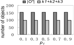
(a) RU

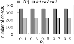
(b) CL

Figure 6: $|\mathscr{O}^{*}|$ and $k_{1}+k_{2}+k_{3}$ vs. $p_{t}$

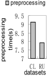
(a)

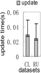
(b)

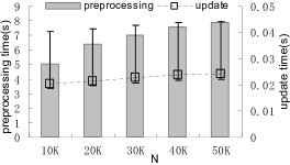
(c)

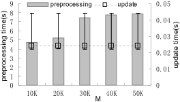
(d)

(e)

Figure 7: Preprocessing and Update Performance

Thus far, all the experiments are based on both real and synthetic data sets. For the two data sets, the preprocessing time and update time are illustrated in Figure 7(a) and 7(b), respectively. The preprocessing process is very fast, it only takes several seconds. (Note: recall Figure 2(d), the time is the hour level if we pre-compute a set of uncertainty regions). Also, the update time is very short, it only takes about tens of milliseconds. In the sequel, we study the impact of $N$, $M$, $\epsilon$ and $\zeta$ on the performance, based on synthetic data sets.

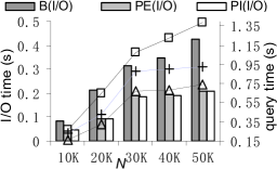
(a) RU (UD)

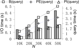
(b) RU (DG)

Figure 8: Query and I/O Efficiency vs. $N$

Effect of $N$. Figure 7(c) and Figure 8 illustrate the experimental results by varying $N$ (the number of moving objects) from $1e+4$ to $5e+4$. From these figures, we can see that the preprocessing time, update time, query time and I/O time increase as $N$ increases. In terms of the query and I/O time, the proposed methods always outperform the B, and the (time) growth rate of the B is significantly faster than the ones of the proposed methods as $N$ increases (especially when $N>3e+4$). This demonstrates that the proposed methods have better scalability.

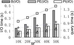
(a) RU (UD)

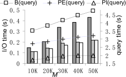
(b) RU (DG)

Figure 9: Query and I/O Efficiency vs. $M$

Effect of $M$. Figure 7(d) and Figure 9 illustrate the results by varying $M$ (the number of restricted areas) from $1e+4$ to $5e+4$. We can see from Figure 7(d) that the preprocessing time increases as $M$ increases, whereas the update time is constant as $M$ increases. This is because the preprocessing process needs to construct ${\mathscr{I}}_{r}$ (the index of restricted areas); the update process however, is irrelevant with ${\mathscr{I}}_{r}$. In addition, Figure 9 shows that both the query and I/O time slightly increase as $M$ increases, and the proposed methods always outperform the B. Similar to the last set of experiments, in terms of the query and I/O time, the growth rate of the B is significantly faster than the proposed methods as $M$ increases. This further demonstrates that the proposed methods have better scalability.

Up to now, we have reported the main experimental results related to the baseline method and proposed methods. We are now ready to investigate the effectiveness of the optimization strategy proposed in Section VI. With regard to explicit and implicit queries, we use respectively the PE$+$O and PI$+$O to denote the algorithms integrated the optimization strategy presented in Section VI, for ease of discussion.

Effectiveness of optimization strategy. Figure 10(a) reports the results when explicit queries are executed. From this figure we can easily see that the I/O time of PE$+$O is obviously less than the one of PE, i.e., the improvement factor is relatively large. This demonstrates that the strategy proposed in Section VI is effective. Note that the query time of PE$+$O is also less than the one of PE (although the improvement factor is not as much as the one for I/O time). Figure 10(b) reports the results when implicit queries are executed, from which we can derive similar findings. We remark that when we vary other parameters (e.g., $\xi$, $N$, $M$) instead of $\zeta$, the experimental results also support our findings, i.e., the PE$+$O (PI$+$O) outperforms the PE (PI), and the improvement factor for I/O time is relatively large. To save space, we here do not plot those results.

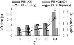
(a) RU dataset (UD)

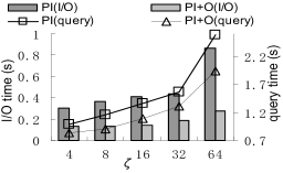
(b) RU dataset (UD)

Figure 10: The effectiveness of optimization

In addition to testing the total I/O time, we also investigate the I/O time for retrieving restricted areas and moving objects, respectively. Figure 11 reports the results when the default settings are used. We can easily see that in terms of PE, most of I/O time are spent on retrieving restricted area data from the database. In contrast, the PE$+$O takes less time to retrieve restricted areas, as the optimization strategy discussed in Section VI avoids to retrieve redundant restricted area data from the database. Another interesting finding is that when the CL data sets are used, the effectiveness of optimization strategy is more obvious. This is because the points (i.e., recorded locations of moving objects) are clustered in the CL data sets, rendering that different candidate moving objects easily share the same restricted areas. We remark that the I/O time of implicit query is the same as the one of explicit query, omitted for saving space.

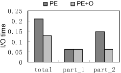
(a) RU

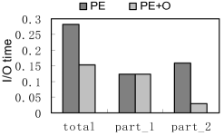
(b) CL

Figure 11: Total I/O time and patial I/O time. In these figures, the term “part$\_$1” denotes the I/O cost for retrieving moving objects, and the term “part$\_$2” denotes the I/O cost for retrieving restricted areas.

Summary. On the whole, these experimental results show us that (i) the proposed algorithms obviously outperform the baseline method regardless of the I/O or query performance; (ii) the proposed algorithms have better scalability, compared to the baseline method; (iii) while the I/O performance of two proposed algorithms is identical, they have different query performance (it is consistent with our theoretical analysis); (iv) the preprocessing process is fast and the update efficiency is high; (v) the optimization strategy (discussed in Section VI) can significantly improve the I/O efficiency, and also reduce the query time although the improvement factor is not very large. Furthermore, these experimental results also demonstrate the robustness and flexibility of our methods.

VIII Concluding remarks

In this paper, we discussed the CSPTRQ for moving objects. We differentiated two forms of CSPTRQs: explicit and implicit ones (as they can have different solutions, performance results, and purposes/applications). We showed the challenges, and proposed efficient solutions that are easy-to-understand and also easy-to-implement. Interestingly, the initial idea of our solutions is inspired by a casual trifle — shopping in a supermarket. In brief, to answer the explicit query, we incorporated two main ideas: swapping the order of geometric operations; and computing the probability using a multi-step mechanism. We then extended these ideas to answer the implicit query, in which an enhanced multi-step mechanism is naturally developed. Furthermore, we developed a novel strategy used to retrieving restricted areas in a more efficient manner. While the rationales behind our solutions are simple, extensive experimental results demonstrated the effectiveness and efficiency of the proposed algorithms. Meanwhile, from the experiential results, we further perceived the difference between explicit and implicit queries; this interesting finding is meaningful for the future research. In the future, we prepare to study other types of probabilistic threshold queries (e.g., concurrent queries, kNN queries) while considering the existence of restricted areas (i.e., obstacles). Another interesting research topic is to extend the concept of restricted areas to other uncertainty models.

References

- [1] P.-A. Albinsson and S. Zhai. High precision touch screen interaction. In International Conference on Human Factors in Computing Systems (CHI), pages 105–112. 2003.
- [2] S. Chaudhuri, G. Das, V. Hristidis, and G. Weikum. Probabilistic ranking of database query results. In International Conference on Very Large Data Bases (VLDB), pages 888–899. 2004.
- [3] M. A. Cheema, L. Brankovic, X. Lin, W. Zhang, and W. Wang. Multi-guarded safe zone: An effective technique to monitor moving circular range queries. In IEEE International Conference on Data Engineering (ICDE), pages 189–200. 2010.
- [4] J. Chen and R. Cheng. Efficient evaluation of imprecise location dependent queries. In IEEE International Conference on Data Engineering (ICDE), pages 586–595. 2007.
- [5] R. Cheng, L. Chen, J. Chen, and X. Xie. Evaluating probability threshold k-nearest-neighbor queries over uncertain data. In International Conference on Extending Database Technology (EDBT), pages 672–683. 2009.
- [6] R. Cheng, D. V. Kalashnikov, and S. Prabhakar. Querying imprecise data in moving object environments. IEEE Transactions on Knowledge and Data Engineering (TKDE), 16(9):1112–1127, 2004.
- [7] R. Cheng, Y. Xia, S. Prabhakar, R. Shah, and J. S. Vitter. Efficient indexing methods for probabilistic threshold queries over uncertain data. In International Conference on Very Large Data Bases (VLDB), pages 876–887. 2004.
- [8] B. S. E. Chung, W.-C. Lee, and A. L. P. Chen. Processing probabilistic spatio-temporal range queries over moving objects with uncertainty. In International Conference on Extending Database Technology (EDBT), pages 60–71. 2009.
- [9] B. Cui, D. Lin, and K.-L. Tan. Impact: A twin-index framework for efficient moving object query processing. Data and Knowledge Engineering (DKE), 59(1):63–85, 2006.
- [10] A. L. Duwaer. Data processing system with a touch screen and a digitizing tablet, both integrated in an input device. US Patent, 5231381, 1993.
- [11] Y. Gao and B. Zheng. Continuous obstructed nearest neighbor queries in spatial databases. In ACM International Conference on Management of Data (SIGMOD), pages 577–589. 2009.
- [12] B. Gedik, K.-L. Wu, P. S. Yu, and L. Liu. Processing moving queries over moving objects using motion-adaptive indexes. IEEE Transactions on Knowledge and Data Engineering (TKDE), 18(5):651–668, 2006.
- [13] M. O. Hofmann, A. McGovern, and K. R. Whitebread. Mobile agents on the digital battlefield. In Agents, pages 219–225. 1998.
- [14] H. Hu, J. Xu, and D. L. Lee. A generic framework for monitoring continuous spatial queries over moving objects. In ACM International Conference on Management of Data (SIGMOD), pages 479–490. 2005.
- [15] M. Hua, J. Pei, W. Zhang, and X. Lin. Ranking queries on uncertain data: a probabilistic threshold approach. In ACM International Conference on Management of Data (SIGMOD), pages 673–686. 2008.
- [16] K. A. D. Jong. Evolutionary computation: a unified approach. MIT Press, Cambridge MA, 2006.
- [17] B. Kuijpers and W. Othman. Trajectory databases: Data models, uncertainty and complete query languages. Journal of Computer and System Sciences (JCSS), 76(7):538–560, 2010.
- [18] M. F. Mokbel and W. G. Aref. Sole: scalable on-line execution of continuous queries on spatio-temporal data streams. The VLDB Journal (VLDB J.), 17(5):971–995, 2008.
- [19] M. F. Mokbel, X. Xiong, and W. G. Aref. Sina: Scalable incremental processing of continuous queries in spatio-temporal databases. In ACM International Conference on Management of Data (SIGMOD), pages 623–634. 2004.
- [20] H. Mokhtar, J. Su, and O. H. Ibarra. On moving object queries. In International Symposium on Principles of Database Systems (PODS), pages 188–198. 2002.
- [21] R. R. Murphy. Disaster Robotics. The MIT Press, Cambridge, 2014.
- [22] D. Olteanu and H. Wen. Ranking query answers in probabilistic databases: Complexity and efficient algorithms. In IEEE International Conference on Data Engineering (ICDE), pages 282–293. 2012.
- [23] D. Pfoser and C. S. Jensen. Capturing the uncertainty of moving-object representations. In International Symposium on Advances in Spatial Databases (SSD), pages 111–132. 1999.
- [24] S. Prabhakar, Y. Xia, D. V. Kalashnikov, W. G. Aref, and S. E. Hambrusch. Query indexing and velocity constrained indexing: Scalable techniques for continuous queries on moving objects. IEEE Transaction on Computers (TC), 51(10):1124–1140, 2002.
- [25] Y. Qi, R. Jain, S. Singh, and S. Prabhakar. Threshold query optimization for uncertain data. In ACM International Conference on Management of Data (SIGMOD), pages 315–326. 2010.
- [26] D. Sidlauskas, S. Saltenis, and C. S. Jensen. Parallel main-memory indexing for moving-object query and update workloads. In ACM International Conference on Management of Data (SIGMOD), pages 37–48. 2012.
- [27] A. P. Sistla, O. Wolfson, S. Chamberlain, and S. Dao. Modeling and querying moving objects. In IEEE International Conference on Data Engineering (ICDE), pages 422–432. 1997.
- [28] A. P. Sistla, O. Wolfson, S. Chamberlain, and S. Dao. Querying the uncertain position of moving objects. In Temporal Databases, pages 310–337. 1997.
- [29] W. Sun, C. Chen, B. Zheng, C. Chen, L. Zhu, W. Liu, and Y. Huang. Merged aggregate nearest neighbor query processing in road networks. In ACM Conference on Information and Knowledge Management (CIKM), pages 2243–2248. 2013.
- [30] Y. Tao, R. Cheng, X. Xiao, W. K. Ngai, B. Kao, and S. Prabhakar. Indexing multi-dimensional uncertain data with arbitrary probability density functions. In International Conference on Very Large Data Bases (VLDB), pages 922–933. 2005.
- [31] Y. Tao, D. Papadias, and J. Sun. The tpr*-tree: An optimized spatio-temporal access method for predictive queries. In International Conference on Very Large Data Bases (VLDB), pages 790–801. 2003.
- [32] Y. Tao, X. Xiao, and R. Cheng. Range search on multidimensional uncertain data. ACM Transactions on Database Systems (TODS), 32(3), 2007.
- [33] G. Trajcevski. Probabilistic range queries in moving objects databases with uncertainty. In International ACM Workshop on Data Engineering for Wireless and Mobile Access (MobiDE), pages 39–45. 2003.
- [34] G. Trajcevski, A. N. Choudhary, O. Wolfson, L. Ye, and G. Li. Uncertain range queries for necklaces. In International Conference on Mobile Data Management (MDM), pages 199–208. 2010.
- [35] G. Trajcevski, O. Wolfson, K. Hinrichs, and S. Chamberlain. Managing uncertainty in moving objects databases. ACM Transactions on Database Systems (TODS), 29(3):463–507, 2004.
- [36] H. Wang and R. Zimmermann. Processing of continuous location-based range queries on moving objects in road networks. IEEE Transactions on Knowledge and Data Engineering (TKDE), 23(7):1065–1078, 2011.
- [37] Z.-J. Wang, D.-H. Wang, B. Yao, and M. Guo. Probabilistic range query over uncertain moving objects in constrained two-dimensional space. IEEE Transactions on Knowledge and Data Engineering (TKDE), 27(3):866–879, 2015.
- [38] O. Wolfson, A. P. Sistla, S. Chamberlain, and Y. Yesha. Updating and querying databases that track mobile units. Distributed and Parallel Databases (DPD), 7(3):257–387, 1999.
- [39] O. Wolfson, B. Xu, S. Chamberlain, and L. Jiang. Moving objects databases: Issues and solutions. In International Conference on Scientific and Statistical Database Management (SSDBM), pages 111–122. 1998.
- [40] K.-L. Wu, S.-K. Chen, and P. S. Yu. Incremental processing of continual range queries over moving objects. IEEE Transactions on Knowledge and Data Engineering (TKDE), 18(11):1560–1575, 2006.
- [41] Y. Yuan, L. Chen, and G. Wang. Efficiently answering probability threshold-based shortest path queries over uncertain graphs. In International Conference on Database Systems for Advanced Applications (DASFAA), pages 155–170. 2010.
- [42] M. Zhang, S. Chen, C. S. Jensen, B. C. Ooi, and Z. Zhang. Effectively indexing uncertain moving objects for predictive queries. Proceedings of the VLDB Endowment (PVLDB), 2(1):1198–1209, 2009.
- [43] R. Zhang, H. V. Jagadish, B. T. Dai, and K. Ramamohanarao. Optimized algorithms for predictive range and knn queries on moving objects. Information Systems (IS), 35(8):911–932, 2010.
- [44] Y. Zhang, X. Lin, Y. Tao, W. Zhang, and H. Wang. Efficient computation of range aggregates against uncertain location-based queries. IEEE Transactions on Knowledge and Data Engineering (TKDE), 24(7):1244–1258, 2012.
- [45] K. Zheng, G. Trajcevski, X. Zhou, and P. Scheuermann. Probabilistic range queries for uncertain trajectories on road networks. In International Conference on Extending Database Technology (EDBT), pages 283–294. 2011.