Inflation in the Generalized Inverse Power Law Scenario

Abstract

We propose a single field inflationary model by generalizing the inverse power law potential from the intermediate model. We study the implication of our model on the primordial anisotropy of cosmological microwave background radiation. Specifically, we apply the slow-roll approximation to calculate the scalar spectral tilt $n_{s}$ and the tensor-to-scalar ratio $r$. The results are compared with the recent data measured by the Planck satellite. We found that by choosing proper values for the parameters, our model can well describe the Planck data.

1 Introduction

Cosmological inflation [1, 2, 3, 4] has been recognized as a compelling attempt to solve several puzzles of standard Big Bang cosmology, such as the flatness, horizon and monopole problems. In a modern view, the most important property of inflation is its ability to generate primordial anisotropy in the early universe [5, 6, 7], which is the necessary initial condition leading to the structure formation. Recently the observation on the anisotropy of cosmological microwave background (CMB) radiation by the Planck satellite [8] provides unprecedent precision data on the primordial density fluctuation. After combined with WMAP large-angle polarization data, the best fit of the scaler spectral index obtained by Planck is

$$n_{s}=0.9603\pm 0.0073,$$

Furthermore, Planck reveals the tensor-to-scalar ratio $r<0.11$ at the 95% CL. The Planck data indicate that exact scale invariance is ruled out at over 5$\sigma$, as well as that the gravitational wave contribution is small compared to the scalar contribution. These measurements set stringent constraints on the parameter space of various inflationary models, which can be discriminated by the Planck data. Strikingly, it is found that the earliest inflationary model, the $R^{2}$ inflation [1, 9], is fully consistent with the Planck data (see also its connection to the conformal invariant supergravity theory in Ref. [10]). However, some well motivated inflationary models are found to be in conflict with the Planck data. A renowned example is the original chaotic inflation [11], which is disfavored at 95% CL. Different approaches have been proposed to reconcile the models with the Planck data, such as introducing non-minimal coupling to gravity [12], or choosing the non-Bunch-Davis vacuum [13].

In this work, we consider an alternative single field inflationary model, motivated by the intermediate model [14, 15, 16] which contains only the inverse power law term:

$$V(\phi)=\Lambda^{4}\left(M_{pl}\over\phi\right)^{\beta},$$ (1.1)

with $\beta>0$. A notable feature of intermediate model is that it leads to exact solution to the equation of motion. Like many other models, the inverse power law potential is disfavored by the Planck data, being outside the joint 95% CL contour of $n_{s}$ and $r$ for any $\beta$. However, as we will show blow, after slightly modifying the original model, we find that the new form of potential, as a generalization of the inverse power law potential, can well describe the Planck $n_{s}$ and $r$ data.

2 Generalizing the inverse power law potential

Inflation is driven by the material with the unusual property of a negative pressure. This can be realized by a homogeneous scalar field $\phi=\phi(t)$, the inflaton, whose evolution is governed by the equation of motion

$$\ddot{\phi}+3H\dot{\phi}+V^{\prime}=0,$$ (2.1)

and the Friedmann equation

$$H^{2}={1\over 3M_{pl}^{2}}\left(V(\phi)+{1\over 2}\dot{\phi}^{2}\right),$$ (2.2)

where $M_{pl}=1/\sqrt{8\pi G}$ is the reduced Planck mass, $V(\phi)$ is the potential of the scalar field, and the prime denotes the derivative with respect to the scalar field $\phi$.

With quantum fluctuation, the scalar field is perturbed around its homogenous background

$$\phi(\bm{x},t)=\phi_{0}(t)+\delta\phi(\bm{x},t),$$ (2.3)

where $\phi_{0}(t)$ is the homogenous part of the inflaton. The Fourier modes of the inflaton fluctuation in the uniform curvature gauge obey the following evolution equation [17, 18]

$$(a\delta\phi_{k})^{\prime\prime}+\left(k^{2}-{z^{\prime\prime}\over z}\right)(a\delta\phi_{k})=0$$ (2.4)

here the primes denote the derivative with respect to conformal time, $\delta\phi_{k}$ are the Fourier modes of $\delta\phi$ with the wavevector $\bm{k}$, and $z=a\dot{\phi}/H$.

The potential of the model we consider is sketched as

$$V(\phi)=V_{0}\left(1-\mu\left({M_{pl}\over\phi}\right)^{\beta}\right)^{2},$$ (2.5)

where $\beta$ is a positive integer, and $\mu$ is a positive dimensional-less coefficient. Since the potential (2.5) has inverse power terms and a constant term, we call it as the generalization of the inverse power law potential. At the region $M_{pl}\ll\phi$, the potential in Eq. (2.5) is simplified to

$$V(\phi)\approx V_{0}\left(1-2\mu\left({M_{pl}\over\phi}\right)^{\beta}\right).$$ (2.6)

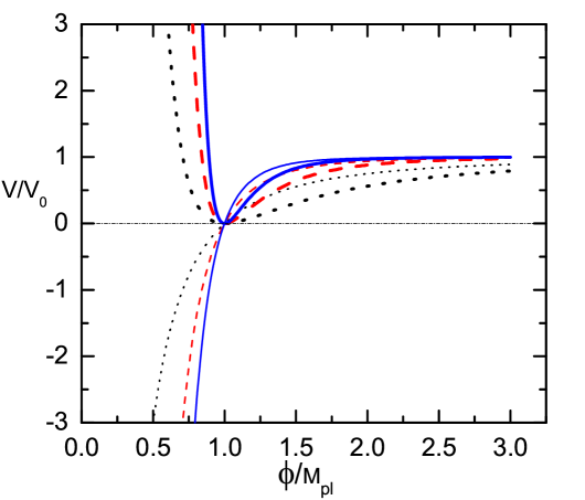
Figure 1: Comparisons between the potential in our model (thick lines) and that in the mutated hybrid inflationary model(thin lines). The dotted, dashed, and solid lines correspond to $\beta=2,4$ and 6, respectively. To obtain these curves we simply choose $\mu=1$ for illustration.

In the case of $\beta=2$ or $4$, the form of the potential in (2.6) is similar to the potentials led from some mutated hybrid inflationary models [19, 20]. It is worthwhile to point out that the potential in (2.6) is also motivated by the brane inflation [21, 22, 23]. However, in the region where $\phi$ is comparable with or smaller than $\mu^{1\over\beta}M_{pl}$, the shape of the potential in (2.5) is very different from that in (2.6). In Figure. 1, we plot the shape of the potentials in (2.5) and (2.6), respectively. To obtain these curves we simply choose $\mu=1$ for illustration. In the case of (2.5), the potential has a minimum at $\phi=\mu^{1\over\beta}M_{pl}$, corresponding to the vacuum expectation value (vev) of $\phi$, where the potential vanishes. Therefore, in our model inflation starts from the region where $\phi$ is several times larger than $\mu^{1\over\beta}M_{pl}$, then naturally ends when the minimum is approached. In this letter we utilize the standard technique for analyzing inflation, the so called slow-roll approximation. In this paradigm the $\ddot{\phi}$ term in Eq. (2.1) and the $\dot{\phi}^{2}$ term in Eq. (2.2) are ignored. For this approximation to be valid, the following condition should be satisfied [24, 25]

$$\epsilon(\phi) ={M_{pl}^{2}V^{\prime 2}\over 2V^{2}}\ll 1,$$ (2.7)

$$|\eta(\phi)| =\left|{M_{pl}^{2}V^{\prime\prime}\over V}\right|\ll 1.$$ (2.8)

Using the potential given in (2.5), we obtain the corresponding slow-roll parameters as

$$\epsilon ={2\mu^{2}\beta^{2}\left({M_{pl}\over\phi}\right)^{2\beta+2}\over\left(1-\mu\left({M_{pl}\over\phi}\right)^{\beta}\right)^{2}},$$ (2.9)

$$\eta ={2\mu^{2}\beta^{2}\left({M_{pl}\over\phi}\right)^{2\beta+2}\over\left(1-\mu\left({M_{pl}\over\phi}\right)^{\beta}\right)^{2}}-{2(\beta+1)\beta\mu\left({M_{pl}\over\phi}\right)^{\beta+2}\over 1-\mu\left({M_{pl}\over\phi}\right)^{\beta}}.$$ (2.10)

In our model, inflation starts at the region $\mu(M_{pl}/\phi)^{\beta}\ll 1$, where the slow-roll approximation is valid. Therefore the above two parameters can be simplified to

$$\epsilon \approx 2\mu^{2}\beta^{2}\left({M_{pl}\over\phi}\right)^{2\beta+2},$$

$$\eta \approx-2(1+\beta)\beta\mu\left({M_{pl}\over\phi}\right)^{\beta+2}.$$ (2.11)

We can see that the two parameters satisfy $\epsilon<|\eta|\ll 1$ in the slow-roll limit, also in our model $\eta$ is negative.

3 Spectral tilt and scalar-to-tensor ratio from the model

Usually the scale dependence of the power spectra of curvature and tensor perturbations are defined as

$$\mathcal{P}_{\mathcal{R}}(k) =A_{s}\left({k\over k_{*}}\right)^{n_{s}-1+{1\over 2}\textrm{d}n_{s}/d\ln k\ln(k/k_{*})+\cdots},$$ (3.1)

$$\mathcal{P}_{t}(k) =A_{t}\left({k\over k_{*}}\right)^{n_{t}+{1\over 2}\textrm{d}n_{t}/d\ln k\ln(k/k_{*})+\cdots},$$ (3.2)

where $A_{s}$ ($A_{t}$) is the scalar (tensor) amplitude, $n_{s}$ ($n_{t}$) is the scalar (tensor) spectral index, and $\textrm{d}n_{s}/d\ln k(\textrm{d}n_{t}/d\ln k)$ is the running of the scalar (tensor) spectral index, respectively. Here we mainly focus on the scalar spectral tilt $n_{s}$, and the tensor-to-scalar ratio $r$ at the pivot scale. They can be expressed by the slow-roll parameters at the leading order as:

$$n_{s}-1 \approx 2\eta-6\epsilon,$$ (3.3)

$$r ={\mathcal{P}_{t}(k_{*})\over\mathcal{P}_{\mathcal{R}}(k_{*})}\approx 16\epsilon.$$ (3.4)

The slow-roll parameters are determined by the value of the inflation field $\phi_{*}$ where the comoving scale $k_{*}=a_{*}H_{*}$ crosses the Hubble radius for the first time. To resolve $\phi_{*}$ the slow-roll approximation is usually used to calculate the number of e-foldings after the horizon exit

$$N_{*}=\int_{t_{*}}^{t_{\textrm{end}}}Hdt\approx{1\over M_{pl}^{2}}\int_{\phi_{\textrm{end}}}^{\phi_{*}}{V\over V^{\prime}}d\phi,$$ (3.5)

where the subscript “end" denotes the end of the inflation defined by $\epsilon(\phi_{\textrm{end}})=1$.

Using the potential (2.5) in our model, we obtain the number of e-foldings as

$$N_{*} ={2\left({\phi_{*}\over M_{pl}}\right)^{\beta+2}-\mu(\beta+2)\left({\phi_{*}\over M_{pl}}\right)^{2}\over 4\mu\beta(\beta+2)}$$ (3.6)

$$\approx{\left({\phi_{*}\over M_{pl}}\right)^{\beta+2}\over 2\mu\beta(\beta+2)},$$ (3.7)

where the main contribution to $N_{*}$ in the integration (3.5) comes from the upper limit $\phi_{*}$. Therefore we obtain the slow-roll parameters at the pivot scale:

$$\epsilon(\phi_{*}) =2\mu^{2\over\beta+2}\beta^{2}\left[2N\beta(\beta+2)\right]^{-{2\beta+2\over\beta+2}},$$ (3.8)

$$\eta(\phi_{*}) =-{(\beta+1)\over(\beta+2)N_{*}}.$$ (3.9)

Using the above results, the scalar spectral index $n_{s}$ can be expressed as

$$n_{s} \approx 1-{2(\beta+1)\over(\beta+2)N_{*}},$$ (3.10)

which is independent of parameter $\mu$. In the limit $\beta\rightarrow\infty$, the spectral index turns to $n_{s}=1-{2\over N_{*}}$, mimicking the results in the $R^{2}$ inflationary model. Practically, for the model being consistent with the Planck data, we do not need to push $\beta\rightarrow\infty$. In the case of number of e-foldings $N_{*}=55$, We find that for $\beta=4$, our model leads to $n_{s}=0.9698$, which is already consistent with the Planck+WP data ($n_{s}=0.9624\pm 0.0075$) after the possible tensor component is included.

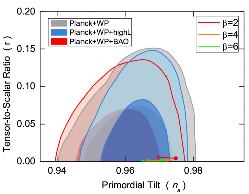
Figure 2: Prediction of $n_{s}$ and $r$ for $\beta=2,4$ and 6 compared to Marginalized joint 68% and 95% CL regions from Planck [8] in combination with WP, highL and BAO data sets. The smaller and larger circles correspond to the results for $N_{*}=50$ and $N_{*}=60$, respectively.

The scalar-to-tensor ratio

$$r =32\mu^{2\over\beta+2}\beta^{2}\left[2N_{*}\beta(\beta+2)\right]^{-{2\beta+2\over\beta+2}},$$ (3.11)

depends both on $\beta$ and $\mu$. However, because of the appearance of the factor $\mu^{2\over\beta+2}$, the dependence of $r$ on $\mu$ may be weak at large $\beta$. For example, in the case of $\beta=6$, when $\mu$ varies between $10^{-4}$ and $10^{4}$, the factor $\mu^{2\over\beta+2}$ varies between 0.1 and 10. Actually, in the limit $\beta\rightarrow\infty$, the dependence of $r$ on $\mu$ disappears, and $r\rightarrow 8/(N_{*}^{2}\beta^{2})\simeq 0$. Therefore, in this limit, although the scalar spectral index $n_{s}$ agrees with the $R^{2}$ model predictions, the tensor-to-scalar ratio $r$ does not, as the $R^{2}$ model predicts that $r\simeq 12/N_{*}^{2}$. To give a robust prediction on $r$ at finite $\beta$, we still need to determine the value or the range of parameter $\mu$. We argue that adopting $\mu\approx 1$ is a natural choice. This corresponds that the inflaton has a vev at $\phi\approx M_{pl}$. Using the COBE normalization [26]

$${V^{1/4}\over\epsilon^{1/4}}=6.6\times 10^{16}\,\textrm{GeV},$$ (3.12)

we find that the potential at the pivot scale $V_{*}$, or equivalently, the parameter $V_{0}$ are constrained as $0.45\times 10^{16}\,\textrm{GeV}<V_{*}\approx V_{0}<0.85\times 10^{16}\,\textrm{GeV}$ for $\beta$ between 2 and 6.

In Figure. 2, we present the prediction on $n_{s}$ and $r$ from our model for $\beta=2$ (red line), 4 (orange line) and 6 (blue line). The smaller and larger circles correspond to $N_{*}=50$ and $60$, respectively. The prediction is compared to the marginalized joint 68% and 95% CL regions from Planck in combination with WP, highL or BAO data sets. From the figure one can see that our model predictions for $\beta=2,4$ and $6$ are inside the 95% CL regions of all data sets. Especially, for $\beta=6$, the result is well consistent with the Planck constraints. Numerical study shows that at the pivot scale, the size of the inflationary field is $\phi_{*}\approx 5.5M_{pl}$, $3.7M_{pl}$ and $2.9M_{pl}$ for $\beta=2$, 4 and $6$, respectively.

$\beta=4$	$\beta=6$
$\mu$ 1 $10^{2}$ $10^{3}$ $n_{s}$  0.9698  0.9700   0.9700 $r$  0.0010   0.0044  0.0089	$\mu$ 1 $10^{2}$ $10^{4}$ $n_{s}$  0.9682  0.9684   0.9686 $r$  0.0004   0.0011  0.0033

Table 1: Numerical results for $n_{s}$ and $r$ with $\mu$ varied from 1 to $10^{3}$ (for $\beta=4$) or 1 to $10^{4}$ (for $\beta=6$), The number of e-foldings after the horizon exit chosen in this calculation is $N_{*}=55$.

Our model predicts rather small gravitational wave contribution for $\mu=1$ at large $\beta$. In order to figure out if gravitational wave contribution is detectable at large $\beta$, we study the dependence of $r$ on the parameter $\mu$. We vary the value of $\mu$ for fixed $N_{*}=55$ and show the corresponding results in Table. 1. We find that as $\mu$ increases from 1 to $10^{3}$ (for $\beta=4$ ) or $10^{4}$ (for $\beta=6$), the tensor-to-scalar ratio $r$ increases almost one order of magnitude. Thus the gravitational wave contribution might be detected at the region $\mu$ is several order of magnitude larger than unity for $\beta=6$. We refrain to present the result at larger $\mu$ region, because a larger $\mu$ will give a relative large vev $\mu^{1\over\beta}M_{pl}$; therefore, the inflation should start at the region where $\phi\gg M_{pl}$, which is very unnatural.

Finally, we consider the extreme case when the parameter $\beta$ approaches to 0. In this limit the potential $V$ does not depend on $\phi$, thus the derivative $V^{\prime}$ and $V^{\prime\prime}$ vanish. As a consequence, the slow-roll parameters are zero in this case, leading to $n_{s}=1$ and $r=0$. Therefore, the extreme case $\beta\sim 0$ is ruled out by the Planck data.

4 conclusion

We have studied a class of inflationary models which are generalized from the inverse power law potential. We presented the model prediction on the scalar spectral tilt $n_{s}$ and the tensor-to-scalar ratio $r$. We found that in the case of $\beta=6$, the model is well consistent with the Planck data. Our model predicts rather small tensor-to-scalar for $\mu$ around unity. The parameter $\mu$ is loosely bounded by the Planck data, such that the varying of $\mu$ from 1 to $10^{4}$ leads to $r$ changing an order of magnitude (for $\beta=6$). Future precision measurement on the tensor-to-scalar could be used to pin down the range of the model parameters.

References

- [1] A. A. Starobinsky, “A New Type of Isotropic Cosmological Models Without Singularity,” Phys. Lett. B 91, 99 (1980).
- [2] A. H. Guth, “The Inflationary Universe: A Possible Solution to the Horizon and Flatness Problems,” Phys. Rev. D 23, 347 (1981).
- [3] A. Albrecht and P. J. Steinhardt, “Cosmology for Grand Unified Theories with Radiatively Induced Symmetry Breaking,” Phys. Rev. Lett. 48, 1220 (1982).
- [4] A. D. Linde, “A New Inflationary Universe Scenario: A Possible Solution of the Horizon, Flatness, Homogeneity, Isotropy and Primordial Monopole Problems,” Phys. Lett. B 108, 389 (1982).
- [5] A.D. Linde, Particle Physics and Infationary Cosmology, Harwood, Chur, Switzerland (1990).
- [6] A.R. Liddle and D.H. Lyth, Cosmological Infation and Large-Scale Structure, Cambridge University Press, Cambridge, England (2000).
- [7] D.H. Lyth and A.R. Liddle, THE Priordial Density Perturbation, Cambridge University Press, Cambridge, England (2009).
- [8] P. A. R. Ade et al. [Planck Collaboration], “Planck 2013 results. XXII. Constraints on inflation,” arXiv:1303.5082 [astro-ph.CO].
- [9] A. A. Starobinsky, “The Perturbation Spectrum Evolving from a Nonsingular Initially De-Sitter Cosmology and the Microwave Background Anisotropy,” Sov. Astron. Lett. 9, 302 (1983).
- [10] R. Kallosh and A. Linde, “Superconformal generalizations of the Starobinsky model,” JCAP 1306, 028 (2013) [arXiv:1306.3214 [hep-th]].
- [11] A. D. Linde, “Chaotic Inflation,” Phys. Lett. B 129, 177 (1983).
- [12] R. Kallosh and A. Linde, “Superconformal generalization of the chaotic inflation model ,” JCAP 1306, 027 (2013) [arXiv:1306.3211 [hep-th]].
- [13] A. Ashoorioon, K. Dimopoulos, M. M. Sheikh-Jabbari and G. Shiu, “Reconciliation of High Energy Scale Models of Inflation with Planck,” arXiv:1306.4914 [hep-th].
- [14] J. D. Barrow, “Graduated Inflationary Universes,” Phys. Lett. B 235, 40 (1990).
- [15] A. G. Muslimov, “On The Scalar Field Dynamics In A Spatially Flat Friedman Universe,” Class. Quant. Grav. 7, 231 (1990).
- [16] J. D. Barrow and A. R. Liddle, “Perturbation spectra from intermediate inflation,” Phys. Rev. D 47, 5219 (1993).
- [17] V. F. Mukhanov, “Quantum Theory of Gauge Invariant Cosmological Perturbations,” Sov. Phys. JETP 67 (1988) 1297.
- [18] M. Sasaki, “Large Scale Quantum Fluctuations in the Inflationary Universe,” Prog. Theor. Phys. 76 (1986) 1036.
- [19] E. D. Stewart, “Mutated hybrid inflation,” Phys. Lett. B 345, 414 (1995) [astro-ph/9407040].
- [20] G. Lazarides, C. Panagiotakopoulos and N. D. Vlachos, “Initial conditions for smooth hybrid inflation,” Phys. Rev. D 54, 1369 (1996).
- [21] G. R. Dvali, Q. Shafi and S. Solganik, “D-brane inflation,” hep-th/0105203.
- [22] G. Shiu and S. H. H. Tye, “Some aspects of brane inflation,” Phys. Lett. B 516, 421 (2001).
- [23] S. Kachru, R. Kallosh, A. D. Linde, J. M. Maldacena, L. P. McAllister and S. P. Trivedi, “Towards inflation in string theory,” JCAP 0310, 013 (2003)
- [24] A. R. Liddle and D. H. Lyth, “COBE, gravitational waves, inflation and extended inflation,” Phys. Lett. B 291, 391 (1992).
- [25] A. R. Liddle and D. H. Lyth, “The Cold dark matter density perturbation,” Phys. Rept. 231, 1 (1993).
- [26] E. F. Bunn, A. R. Liddle and M. J. White, “Four year COBE normalization of inflationary cosmologies,” Phys. Rev. D 54, 5917 (1996); E. F. Bunn and M. J. White, “The Four year COBE normalization and large scale structure,” Astrophys. J. 480, 6 (1997).