Stimulation of a Singlet Superconductivity in SFS Weak Links by Spin–Exchange Scattering of Cooper Pairs

A. V. Samokhvalov^1,4,∗, R. I. Shekhter², A. I. Buzdin³

¹Institute for Physics of Microstructures, Russian Academy of Sciences,
603950 Nizhny Novgorod, GSP-105, Russia
²Department of Physics, University of Gothenburg, SE-412 96 Göteborg, Sweden
³Institut Universitaire de France and University Bordeaux, LOMA UMR-CNRS 5798,
F-33405 Talence Cedex, France
⁴Lobachevsky State University of Nizhny Novgorod, Nizhny Novgorod 603950, Russia
^∗samokh@ipm.sci-nnov.ru

Josephson junctions with a ferromagnetic metal weak link reveal a very strong decrease of the critical current compared to a normal metal weak link. We demonstrate that in the ballistic regime the presence of a small region with a non-collinear magnetization near the center of a ferromagnetic weak link restores the critical current inherent to the normal metal. The above effect can be stimulated by additional electrical bias of the magnetic gate which induces a local electron depletion of ferromagnetic barrier. The underlying physics of the effect is the interference phenomena due to the magnetic scattering of the Cooper pair, which reverses its total momentum in the ferromagnet and thus compensates the phase gain before and after the spin–reversed scattering. In contrast with the widely discussed triplet long ranged proximity effect we elucidate a new singlet long ranged proximity effect. This phenomenon opens a way to easily control the properties of SFS junctions and inversely to manipulate the magnetic moment via the Josephson current.

Mesoscopic properties of nanometer sized conductors are strongly affected by the injection of correlated electrons (Cooper pairs) from superconducting electrodes. While propagating through normal metal such pairs of electrons are able to preserve their superconducting correlation on mesoscopic lengths providing the superconducting current flow through SNS (superconductor-normal metal-superconductor) weak links Barone-Paterno-Physics ; Golubov-Kupriyanov-Ilichev-RMP04 .

Time reversal of electronic states forming a Cooper pair is an important component of the above correlation. Absence of superconducting pairing interaction in a N part of the superconducting SNS device opens a possibility of easy external manipulation of the spin structure of the propagating Cooper pairs. This offers the means for spintronic manipulation of superconducting weak links. The most efficient ”tailoring” of Cooper pairs can be achieved by external in-homogeneity located on a submicron length scale, which is set by superconducting coherence length, determining the scale of spatial correlation of paired electrons. Here we demonstrate that a tip of the magnetic exchange force microscope (MExFM) Kaiser-Wiesendanger-Nature07 ; Wiesendanger-RMP09 , which induces localized in space magnetic exchange fields can play the role of such a local probe for a spin state of superconducting Cooper pairs. Existing experimental evidences of the externally induced exchange fields $h$ in metals of the order of few Xiong-PRL11 ; Hamaya-APL07 or even few tens Pasupathy-Sci04 millielectronvolts place the electronic coupling to such field in a range of energies comparable with (or even exceeding) superconducting energy scale $\sim 1\,\mathrm{meV}$. We will show that the effect of exchange induced gating of Cooper pairs leads to a new phenomenon - stimulation of long- range singlet superconductivity in SFS (superconductor-ferromagnet-superconductor) weak links.

Magnetic exchange interaction in ferromagnetic metals lifts a degeneracy with respect to spin orientation of the electrons, forming a Cooper pair. This leads to different de-Broglie wavelengths of electrons at Fermi surface for spin-up and spin-down orientation and produces a modulation of the Cooper pair wavefunction while propagating along the ferromagnet Demler-PRB97 . As a result an oscillatory damping of the superconducting ordering is known to appear when a ferromagnetic ordering occurs in a normal metal link connecting two S electrodes Buzdin-rew . This phenomenon provides the basis of the $\pi$-junction realization BuzBulPan-JETPL82 ; Ryazanov-PRL01 ; Oboznov-Ryazanov-Buzdin-PRL06 . Considering the quantum mechanics of quasiparticle excitations the exchange field leads to phase difference $\gamma\sim L/\xi_{h}$ gained between the electron- and hole- like parts of the total wave function along a path of the length $L$ Blanter-PRB04 ; Buzdin-PRB11 , where $\xi_{h}=\hbar V_{F}/2h$ is a characteristic length determined by the exchange field ($V_{F}$ is the Fermi velocity).

Measurable quantities should be calculated as superpositions of fast oscillating contributions $e^{i\gamma}$ from different trajectories and, thus, rapidly vanish with the increasing distance from the SF boundary. It should be noted though, that a simple domain structure consisting of two F layers with opposite orientations of exchange field cancels the phase gain $\gamma$ and suppresses the destructive effect of an exchange field Blanter-PRB04 ; Melnikov-Samokhvalov-prl12 . It is clear therefore that by affecting the spin structure of Cooper pairs, one influences the strength and spatial distribution of the proximity effect induced by Cooper pair penetration inside a ferromagnetic metal. It was suggested before that the Cooper pairs of electrons with aligned spins (with equal-spin pairs) can be formed by spatial non-homogeneous magnetization Bergeret-PRL01 ; Kadigrobov-Shekhter-EL01 . Since they bind electrons with exactly the same de-Broglie wave length, these triplet Cooper pairs do not dephase, thereby leading to long-range proximity effect. Singlet Cooper pairs still become ”filtered out” from spatial transfer of superconducting phase coherence due to a strong dephasing effect, occurring in long (as compared with magnetic coherence length $\xi_{h}$) SFS weak links. To observe such a long ranged triplet superconducting current, the SFS junctions with a composite F layers comprising three non-collinear domains, were suggested theoretically Houzet-Buzdin-PRB07 ; Alidoust-Linder-PRB10 ; Volkov-Efetov-PRB10 and realized in recent experiments Robinson-Science10 ; Khaire-Birge-PRL10 . In such a case the triplet component is generated by a thin ferromagnetic domain, located between superconducting lead and a thick central non-collinear domain. The long ranged Josephson current results from the interference between these triplet components, generated by the left and right superconducting leads.

Here we suggest a new way of manipulating the Cooper pairs flow through a ferromagnet, which consists in using a well controlled tip/probe along the supercurrent flow. This corresponds to the case of the composite F layer with a thin domain, located near the center of the junction. In contrast with the situation analyzed in Refs. Houzet-Buzdin-PRB07 ; Alidoust-Linder-PRB10 ; Volkov-Efetov-PRB10 , the triplet superconducting current is absent for this setup but becomes possible a long–ranged singlet proximity effect. As we will show the field generated by the probe induces a special scattering of Cooper pairs which corresponds to exchange spins of two electrons forming a pair. A schematic picture of such scattering is shown in Fig. 1. As we have previously mentioned two electrons forming a singlet Cooper pair have a non-zero total momentum $\hbar\mathbf{q}=\hbar\mathbf{k}_{\uparrow}-\hbar\mathbf{k}_{\downarrow}$ due to the ferromagnetic exchange splitting of the spin subbands ( The modulus of the Fermi wave-vector for electrons with a spin polarized along the field is larger $\left|\mathbf{k}_{\downarrow}\right|>\left|\mathbf{k}_{\uparrow}\right|$ and $\left|\mathbf{q}\right|\sim 1/\xi_{h}$ ). The electrons in a singlet Cooper pair reach the scattering center (spin exchanger) and scatter their spin so that the new total momentum of the Cooper pair $\hbar\mathbf{q}^{\prime}$ is either unchanged $\hbar\mathbf{q}^{\prime}=\hbar\mathbf{q}$ (Fig. 1A) or reversed $\hbar\mathbf{q}^{\prime}=-\hbar\mathbf{q}$ (Fig. 1B) (see the discussion in Methods). In the first case the spin arrangement of a singlet Cooper pair has not changed with respect to the exchange field and there remains a total phase gain $\gamma\sim(d_{1}+d_{3})/\xi_{h}$ which results in a strong suppression of proximity due to the destructive trajectory interference. In the second case the scattered Cooper pair has a reversed spin arrangement and the total phase gain is $\gamma\sim(d_{1}-d_{3})/\xi_{h}$ . As a result, at a symmetric position of the scatterer ($d_{1}=d_{3}$) the total phase gain for a singlet Cooper pair should be cancelled ($\gamma=0$) and the long range singlet superconducting proximity in SFS link becomes possible.

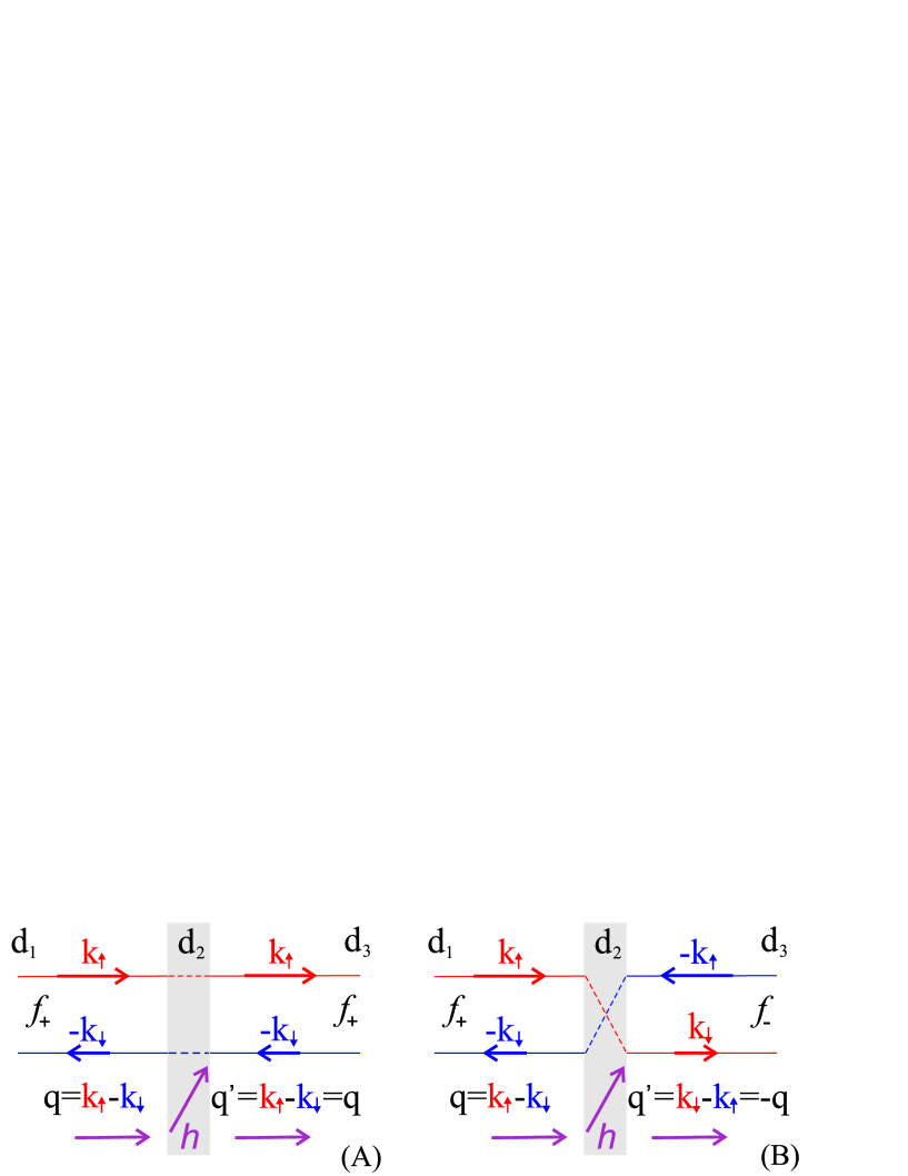
Figure 1: (A) A schematic picture of singlet Cooper pair scattering with no spin–flop transition of electrons. The spin arrangement of a pair $f_{+}$ ($\mathbf{q}=\mathbf{k}_{\uparrow}-\mathbf{k}_{\downarrow}$) does not change with respect to the exchange field: $\mathbf{q}^{\prime}=\mathbf{q}$. (B) A schematic picture of ”exchange” singlet Cooper pair scattering with spin–flop transition of electrons: $f_{+}\rightarrow f_{-}$. The spin arrangement of a pair $f_{-}$ was changed with respect to the exchange field: $\mathbf{q}^{\prime}=\mathbf{k}_{\downarrow}-\mathbf{k}_{\uparrow}=-\mathbf{q}$. The scattering domain $d_{2}$ is shown by grey color. The symbols $f_{\pm}$ indicate the Cooper pairs with zero spin projection and a reversed spin arrangement (see Methods).

To be more precise, we consider the Josephson transport through a normal ballistic nanowire (NW) in contact with a ferromagnetic insulator (FI). The FI turns the NW into an effective ferromagnet with an exchange field $h$. The schematic picture of the SFS device is presented in Fig. 2A. The total length of the constriction $d=d_{1}+d_{2}+d_{3}$ is assumed to be large compared to the magnetic coherence length $\xi_{h}=\hbar V_{F}/2h$: $d\gg\xi_{h}$. For simplicity we restrict ourselves to the case of a short junction with $d\ll\xi_{n}$, where $\xi_{n}=\hbar V_{F}/T_{c}$ is the coherence length of normal metal ($T_{c}$ is the critical temperature of the S layer). The magnetic tip is assumed to bring on localized in space magnetic exchange field inhomogeneity which we model by a stepwise profile:

$$h(z)=\left\{\begin{array}[c]{ccc}h\mathbf{z}_{0},&\mathrm{in\;domains}&d_{1},d_{3}\\ h\left(\mathbf{z}_{0}\cos\alpha+\mathbf{x}_{0}\sin\alpha\right),&\mathrm{in\;domain\;}&d_{2}\,,\end{array}\right.$$ (1)

where $\alpha$ is the angle of the exchange field rotation in the central domain $d_{2}$ (see Fig. 2B).

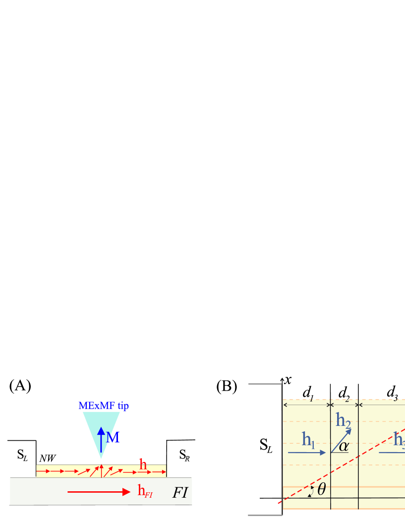
Figure 2: (A) The schematic sketch of the SFS constriction under consideration: normal metal nanowire (NW) in contact with a superconductor (S) and a ferromagnetic insulator (FI). (B) Equivalent SFS Josephson junction containing three ferromagnetic layers (domains) with a stepwise profile of the exchange field (1). Linear quasiparticle trajectory is shown by the red dashed line.

Results

The current–phase relation of SFS Josephson junction is determined by the quasiclassical relation Buzdin-PRB11 ; Melnikov-Samokhvalov-prl12

$$I=\sum\limits_{n}I_{n}=\sum\limits_{n}a_{n}\sin n\varphi\frac{\langle(\mathbf{n},\mathbf{n}_{F})\cos n\gamma\rangle}{\langle(\mathbf{n},\mathbf{n}_{F})\rangle}\ ,$$ (2)

where $\mathbf{n}$ is the unit vector normal to the junction plane, $\mathbf{n}_{F}$ is the unit vector along the trajectory, and $a_{n}$ are the coefficients of the Fourier expansion for the current–phase relation for superconductor–normal metal junction of the same geometry. The angular brackets denote the averaging over different quasiclassical trajectories characterized by a given angle $\theta$ and a certain starting point at the superconductor surface, and for 3D constriction looks as

$$\frac{\langle(\mathbf{n},\mathbf{n}_{F})\cos(n\gamma)\rangle}{\langle(\mathbf{n},\mathbf{n}_{F})\rangle}=2\int\limits_{0}^{\pi/2}d\theta\sin\theta\cos\theta\,\cos(n\gamma)\,,$$ (3)

where $\cos\theta=(\mathbf{n},\mathbf{n}_{F})$. At temperatures $T$ close to $T_{c}$ the current–phase relation (2) is sinusoidal, and the coefficient $a_{1}$ is determined by the following simple relations Melnikov-Samokhvalov-prl12 :

$$a_{1}=\frac{eT_{c}}{8\,\hbar}N\left(\frac{\Delta}{T_{c}}\right)^{2}\,.$$ (4)

Here $\Delta$ is the temperature dependent superconducting gap, The factor $N$ is determined by the number of transverse modes in the junction: $N=s_{0}^{-1}\int ds\int d\mathbf{n}_{F}(\mathbf{n}_{F},\mathbf{n})\sim S/s_{0}$, where $S$ is the junction cross–section area, and $s_{0}^{-1}=(k_{F}/2\pi)^{2}$, where $k_{F}$ is the Fermi momentum.

The phase gain $\gamma$ can be conveniently determined from the Eilenberger—type equations Eilen_1968_eqs if we use a standard parametrization Champel of the anomalous quasiclassical Green function $f=f_{s}+\mathbf{f}_{t}\hat{\sigma}$, where $f_{s}$ ($\mathbf{f}_{t}$) singlet (triplet) parts of the function, respectively, and $\hat{\sigma}$ is a Pauli matrix vector in the spin space. The functions $f_{s}$, $\mathbf{f}_{t}$ satisfy the linearized Eilenberger equations Houzet-Buzdin-PRB07 written for zero Matsubara frequencies

$$-i\hbar V_{F}\partial_{s}f_{s}+2\mathbf{h}\mathbf{f}_{t}=0\ ,\qquad-i\hbar V_{F}\partial_{s}\mathbf{f}_{t}+2f_{s}\mathbf{h}=0\ ,$$ (5)

with the boundary conditions $f_{s}(s=s_{L})=1$, $\mathbf{f}_{t}(s=s_{L})=0$ at the left superconducting electrode (for simplicity we consider the case of the absence of the barriers at the interfaces). The phase gain $\gamma$ along the trajectory in the equivalent SFS junction (Fig. 2B) is determined by the singlet part of the anomalous quasiclassical Green function $f_{s}(s=s_{R})=\cos\gamma$ taken at the right superconducting electrode Melnikov-Samokhvalov-prl12 . Solving the equations (5) for the stepwise profile of the exchange field (1) we find (see Methods):

$$\cos\gamma =\cos\delta_{2}\cos(\delta_{1}+\delta_{3})-\cos\alpha\sin\delta_{2}\sin(\delta_{1}+\delta_{3})$$

$$-\sin^{2}\alpha\,\sin\delta_{1}\sin\delta_{3}(1-\cos\delta_{2})\,,$$ (6)

where $\cos\theta=(\mathbf{n},\mathbf{n}_{F})$ and $\delta_{i}=d_{i}/\xi_{h}\cos\theta$ ($i=1,2,3$). Averaging the expression (Results) over the trajectory direction $\theta$ and neglecting the terms proportional to $\xi_{h}/d\ll 1$, which decrease just as for the case of homogeneous ballistic 3D SFS junction, one arrives at the following long–range (LR) contribution:

$$(\cos\gamma)^{LR}=-\frac{1}{2}\sin^{2}\alpha(1-\cos\delta_{2})\,\cos 2\delta_{z}\,,$$ (7)

where $\delta_{z}=z_{0}/\xi_{h}\cos\theta$ and $z_{0}=(d_{1}-d_{3})/2$ is the shift of the central domain with respect to the weak link center. So, the long–range component of the Josephson current at the first harmonic is determined by the relation:

$$I^{LR}\simeq I_{1}^{LR}=a_{1}T_{1}^{LR}\sin\varphi\,,\qquad T_{1}^{LR}=2\int\limits_{0}^{\pi/2}d\theta\sin\theta\cos\theta\,(\cos\gamma)^{LR}\,.$$ (8)

For a very thin central domain $d_{2}\ll\xi_{h}$ in the center of the NW ($z_{0}=0$) one can easily estimate from (7, 8) the critical current of the SFS junction

$$\mathrm{max}\{I^{LR}\}\approx\frac{I_{0}}{2}\sin^{2}\alpha\left(\frac{d_{2}}{\xi_{h}}\right)^{2}\ln\frac{\xi_{h}}{d_{2}}\,,$$ (9)

where $I_{0}=(eT_{c}N/8\hbar)\left(\Delta/T_{c}\right)^{2}$ – is the critical current of the SNS junction for zero exchange field ($\gamma=0$). We see that the long–ranged critical current reaches the maximum at $\alpha=\pi/2$ and grows with the increase of $d_{2}$ up to $d_{2}\sim\xi_{h}$. Our numerical calculations show that it is maximum for $d_{2}\simeq\mathrm{2.5}\,\xi_{h}$ and may reach $\sim\mathrm{0.7}I_{0}$. Certainly, the above long–range effect in the first harmonic describes the properties of the SFS constriction if contribution of higher harmonics in the current–phase relation (2) is negligible. We present the analysis of the second harmonic effect in the Supplementary information.

Discussion

Figure 3 shows the dependence of the maximal Josephson current $I_{c}^{LR}=a_{1}T_{1}^{LR}$ on the thickness $d_{2}$ of the $90^{o}$ domain ($\alpha=\pi/2$) for different values of the shift of the domain $z_{0}$. Naturally, when the thickness of the central domain $d_{2}$ goes to zero, the long–range effect disappears. We can see from Fig. 3, that the long–range component of the Josephson current $I^{LR}$ coincides approximately with the total supercurrent across the junction (2) until the outer domains are long enough: $d_{1},\,d_{3}\gg\xi_{h}$. The amplitude of $I^{LR}$ depends nonmonotonically on the size of the central domain $d_{2}$ and has the first maximum at $d_{2}\simeq 2.5\xi_{h}$. Interestingly, that the long–range contribution generates a $\pi-$junction ($I^{LR}$ is negative for zero shift of the domain $z_{0}=0$). With the shift of the central domain the junction can be switched from $\pi-$ to $0-$ state.

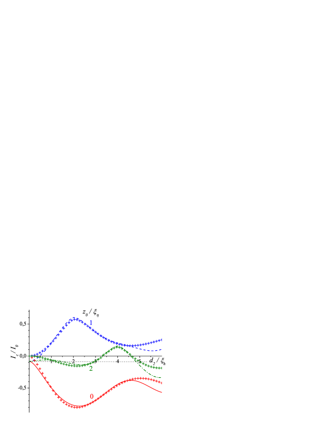
Figure 3: The dependence of maximal Josephson current $I_{c}=\mathrm{max}\{I_{1}\}$ on the thickness $d_{2}$ of the $90^{o}$ domain ($\alpha=\pi/2$) for different values of the shift of the domain $z_{0}$: $z_{0}=0$ - red solid line; $z_{0}=\xi_{h}$ - blue dashed line; $z_{0}=2\xi_{h}$ - green dash-dotted line. Symbols $+$ show the long-range part of the supercurrent. Dotted line shows the value of $I_{c}$ in absence of domain $d_{2}$ ($\alpha=0$). We have set $T=\mathrm{0.9}T_{c}$; $d=20\xi_{h}$ [ $I_{0}=(eT_{c}N/8\hbar)\left(\Delta/T_{c}\right)^{2}$ ].

Figure 4 shows the dependences of the maximal Josephson current $I_{c}$ on the position of the central domain $z_{0}$ for different values of the rotation angle $\alpha$. We may see that the critical current is very sensitive to the position of the central domain and the first zero of $I_{1}$ occurs already at $z_{0}\simeq 0.5\xi_{h}$.

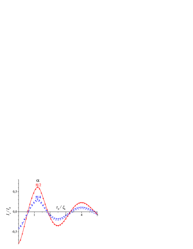
Figure 4: The dependence of maximal Josephson current $I_{c}=\mathrm{max}\{I_{1}\}$ on the shift of the central domain $z_{0}$ for different values of the angle $\alpha$: $\alpha=\pi/2$ - red solid line; $\alpha=\pi/4$ - blue dashed line. Symbols $+$ show the long-range part of the supercurrent. We have set $T=\mathrm{0.9}T_{c}$; $d=20\xi_{h}$; $d_{2}=2.5\xi_{h}$, [ $I_{0}=(eT_{c}N/8\hbar)\left(\Delta/T_{c}\right)^{2}$ ].

Here we considered a simple step–like model of magnetization distribution in F layer. For the very thin central domain $d_{2}\ll\xi_{h}$, we may easily estimate the long ranged contribution $(\cos\gamma)^{LR}\sim\leavevmode\nobreak\ (d_{2}/\xi_{h})^{2}\,(h_{x}/h)^{2}$ which is in accordance with the expression (7). For a general profile of the magnetization it may be convenient to use the transfer–matrix method (see the Supplementary information). The smooth (on the scale $\xi_{h}$) profile of the magnetization decreases the long ranged effect and the proposed mechanism occurs to be most efficient for $d_{2}\sim\xi_{h}$.

Note that the considered phenomenon should generate the oscillating potential profile for the magnetic tip $U(z_{0})\sim-I_{c}(z_{0})\cos\varphi$ which depends on superconducting phase difference across the junction. This opens an interesting possibility to couple the Josephson current oscillations with mechanical modes of the tip. On the other hand the same effect can produce a change of the orientation of the magnetic moment. Inversely, the precession of the magnetic moment shall modulate the critical current of the junction and provides a direct coupling between the superconducting current and the magnetic moment in the weak link similar to the situation discussed in Refs. buzdin-PRL08 ; konschelle-buzdin-PRL09 .

The magnetically tunable long-range SFS proximity effect suggested above has a potential to be an important feature of carbon-based superconducting weak links. Graphene sheets and carbon nanotubes are reported to offer a ballistic propagation for electrons on a micrometer length scale Grushina-APL13 ; Biercuk-CNT . This fact together with appearing reports on a gate tunable magnetism in graphene Candini-NLet11 ; Li-cm13047089 makes all ingredients of the present theory achievable in experiment. Another possibility is to use the indium antimonide ($\mathrm{InSb}$) nanowires as a superconducting weak link. The indium antimonide nanowires, recently used in the experiments to reveal the signature of Majorana fermions Mourik-Sci12 , demonstrated a very high $g-$factor ($g\simeq\mathrm{50}$). Anomalously large g-factor reported in such wires offers the possibility to ”mimic” a ferromagnetic spin-splitting effect of the order of 10 K by simply applying an external magnetic field of the order of 0.1 Tesla, and then making such nanowire a suitable candidate for a weak link to observe the discussed phenomena. Note that in contrast to the experiments Mourik-Sci12 the magnetic field should be applied along the spin-orbit field axis to avoid the interference with the spin-orbit effect.

It should be noted, that new additional functionality of the considered device can be achieved by electric biasing of the magnetic gate Haugen-prb08 ; Semenov-apl07 . In weakly doped ferromagnetic barriers, such bias ($V_{g}$) alters both the charge carrier concentration and the Fermi velocity. Choosing a polarity of electric gating one can create a depletion region beneath the tip. As a result, both the Fermi velocity $V_{F}$ and the exchange length $\xi_{h}=\hbar V_{F}/2h$ decrease in the spatial region of the domain $d_{2}$, and the key parameter responsible for the magnetic exchange scattering $\delta_{2}=d_{2}/\xi_{h}$ grows. For thin domains ($\delta_{2}\ll 1$) the critical current $I_{c}\sim\delta_{2}^{2}$ increases with the gate voltage $V_{g}$, and the local depletion of F barrier should result in the stimulation of the superconductivity. This nontrivial interplay between electric and magnetic gating effects can be used to control singlet Josephson current through ferromagnetic nanowires.

To summarize, we studied the interference phenomena originated by the spin-exchange scattering in ferromagnetic ballistic weak link and demonstrated that they provide an efficient way to control the Josephson current and to couple it with a magnetic moment.

Methods

.1 Transfer–matrix formalism for Eilenberger Equations

To consider the Josephson transport through ferromagnetic layer with a non-collinear magnetizations $\mathbf{M}$ and exchange field $\mathbf{h}$ it is convenient to utilize the transfer–matrix formalism. For this, we need to solve the linearized Eilenberger equations written for zero Matsubara frequencies

$$-i\hbar V_{F}\partial_{s}f_{s}+2\mathbf{h}\mathbf{f}_{t}=0\ ,\quad-i\hbar V_{F}\partial_{s}\mathbf{f}_{t}+2f_{s}\mathbf{h}=0\ ,$$ (10)

for the case when the quantization axis is taken arbitrarily in the ferromagnetic layer of a thickness $d$. We assume that a quasiclassical trajectory $\mathbf{s}$ and exchange field $\mathbf{h}=h\left(\mathbf{z}_{0}\sin\alpha+\mathbf{x}_{0}\cos\alpha\right)$ lie in the plane ($x,\,z$), as shown in Fig. 5.

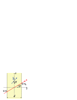
Figure 5: Quasiclassical trajectory $\mathbf{s}$ through homogeneous ferromagnetic layer of a thickness $d$ with an arbitrary direction of the exchange field $\mathbf{h}$.

The trajectory is characterized by a given angle $\theta$ with respect to the $z$-axis. The triplet part $\mathbf{f}_{t}$ of the anomalous quasiclassical Green function $f=f_{s}+\mathbf{f}_{t}\hat{\sigma}$ consists of two nonzero components and can be written as $\mathbf{f}_{t}=f_{tx}\mathbf{x}_{0}+f_{tz}\mathbf{z}_{0}$. Defining the transfer–matrix $\hat{T}_{\alpha}(d,\theta)$ that relates the components of the Green function $f(s)$ at the left ($s=0$) and right ($s=s_{d}=d/\cos\theta$) boundaries of the F layer,

$$\hat{f}(s_{d})=\left(\begin{array}[c]{c}f_{s}(s_{d})\\ f_{tz}(s_{d})\\ f_{tx}(s_{d})\\ \end{array}\right)=\hat{T}_{\alpha}(d,\theta)\left(\begin{array}[c]{c}f_{s}(0)\\ f_{tz}(0)\\ f_{tx}(0)\\ \end{array}\right)\,,$$ (11)

we get the following expression:

$$\hat{T}_{\alpha}(d,\theta)=\left(\begin{array}[c]{ccc}\cos(qs_{d})&-i\cos\alpha\sin(qs_{d})&-i\sin\alpha\sin(qs_{d})\\ -i\cos\alpha\sin(qs_{d})&\sin^{2}\alpha+\cos^{2}\alpha\cos(qs_{d})&\sin\alpha\cos\alpha\left(\cos(qs_{d})-1\right)\\ -i\sin\alpha\sin(qs_{d})&\sin\alpha\cos\alpha\left(\cos(qs_{d})-1\right)&\cos^{2}\alpha+\sin^{2}\alpha\cos(qs_{d})\\ \end{array}\right)\,,$$ (12)

where $q\equiv 1/\xi_{h}=2h/\hbar V_{F}$.

In order to elucidate the peculiarities of the Cooper pairs scattering with a spin-flop transition of electrons it is convenient to introduce the new functions $f_{\pm}=f_{s}\pm f_{tz}$ which describes the pairs with zero spin projection and a reversed spin arrangement. The transfer–matrix $\hat{T}_{\alpha}(d,\theta)$ can be drastically simplified if the direction of the exchange field coincides with a spin quantisation axis $\ \mathbf{z}$. In this case, $\alpha=0$ and $f_{\pm}(s_{d})=\mathrm{e}^{\mp iqs_{d}}f_{\pm}(0)$, $f_{tx}(s_{d})=f_{tx}(0).$ Calculating the superconducting current at the right electrode S_R we readily see that it results from the interference with the singlet component coming from the left electrode $f_{s}(s_{d})=$ $\left(f_{+}(s_{d})+f_{-}(s_{d})\right)/2$ (triplet components are irrelevant because the right electrode provides only the singlet component). The oscillating factors $\mathrm{e}^{\mp iqs_{d}}$ in $f_{\pm}(s_{d})$ produce, after the averaging over the trajectories directions ( angle $\theta$ ), a strong damping of the critical current compared to the normal metal (where these factors are absent).

Now we may easily understand the mechanism of the long-ranged proximity effect. Indeed after coming through the first F layer an extra phase factor appears in $f_{\pm}$ functions (see Fig. 2): $f_{\pm}(s_{d_{1}})=\mathrm{e}^{\mp iqs_{d_{1}}}f_{s}(0)$. In the absence the middle layer, the $f_{\pm}$ at the right electrode would be $f_{\pm}(s_{d_{1}}+s_{d_{3}})=\mathrm{e}^{\mp iq(s_{d_{1}}+s_{d_{3}})}f_{s}(0)$ and the oscillating factors will strongly damp critical current. The additional non-collinear middle layer $d_{2}$ will mix up the components $f_{+}$ and $f_{-}$ - see the matrix (16) and, for example, $f_{+}(s_{d_{1}}+s_{d_{2}})$ in addition to $\mathrm{e}^{-iqs_{d_{1}}}f_{s}(0)$ component will have a $\mathrm{e}^{+iqs_{d_{1}}}f_{s}(0)$ contribution, i. e.  $f_{+}(s_{d_{1}}+s_{d_{2}})=a\,\mathrm{e}^{-iqs_{d_{1}}}\,+\,b\,\mathrm{e}^{+iqs_{d_{1}}}$. In fact, namely this mechanism is schematically presented in the Fig. 1(b). Then the resulting  $f_{+}$ function at the right electrode should be $f_{+}(s_{d_{1}}+s_{d_{2}}+s_{d_{3}})=a$ $\mathrm{e}^{-iq(s_{d_{1}}+s_{d_{3}})}+b\mathrm{e}^{+iq(s_{d_{1}}-s_{d_{3}})}$ and for $d_{1}=d_{3\text{ \ \ }}$

the oscillating factor at the second term vanishes. This means the emergence of the long-ranged singlet proximity effect discussed in the present report. Note that the additional noncollinear F layer $d_{2}$ may strongly increase the critical current, provided that it is placed at the center of the structure.

The transfer–matrix method is very convenient for the calculation of the Josephson transport through the SFS junction containing three ferromagnetic layers with a stepwise profile of exchange field. For this geometry shown in Fig. 2B of the Letter, the anomalous quasiclassical Green function $\hat{f}(s_{R})=(f_{s}(s_{R}),\,f_{tz}(s_{R}),\,f_{tx}(s_{R}))$ at the right superconducting electrode ($s=s_{R}=d/\cos\theta$) can be easily expressed via the boundary conditions $\hat{f}(0)=(1,\,0,\,0)$ at the left superconducting electrode ($s=0$) as follows:

$$\hat{f}(s_{R})=\hat{T}_{0}(d_{3},\theta)\,\hat{T}_{\alpha}(d_{2},\theta)\,\hat{T}_{0}(d_{1},\theta)\hat{f}(0)\,,$$ (13)

where $d=d_{1}+d_{2}+d_{3}$ is the total thickness of the ferromagnetic barrier. As a result, the singlet part $f_{s}(s_{R})$ responsible for the Josephson current through the junction, can be written in the form (Results).

Acknowledgments
The authors thank A.S. Mel’nikov for stimulating discussions. This work was supported, in part, by European IRSES program SIMTECH (contract n.246937), by French ANR grant ”MASH”, by the Swedish VR, by the Russian Foundation for Basic Research (n.13-02-97126), and by the program ”Quantum Mesoscopic and Disordered Structures” of the Russian Academy of Sciences.

Supplementary Information

Supplementary Note 1: Second harmonic contribution
The long–range behavior can be observed for a second harmonic in the current–phase relation

$$I=\sum\limits_{n}I_{n}=\sum\limits_{n}I_{cn}\sin n\varphi$$ (14)

as well. Calculating the $\cos(2\gamma)=2\cos^{2}\gamma-1$ we find the terms which are responsible for a long–range contribution to the supercurrent:

$$(\cos 2\gamma)^{LR}=-\sin^{2}\alpha\left(1-\cos\delta_{2}\right)\times$$ (15)

$$\qquad\left[1-\frac{1}{2}\sin^{2}\alpha\left(1-\cos\delta_{2}\right)\left(1+\frac{1}{2}\cos(4\delta_{z})\right)\right]\,,$$

Averaging over different quasiclassical trajectories for 3D junction we find a nonvanishing long–range supercurrent at the second harmonic:

$$I_{2}^{LR}=|a_{2}|T_{2}\,\sin 2\varphi\,,\quad T_{2}\approx-2\int\limits_{0}^{\pi/2}d\theta\sin\theta\cos\theta\,(\cos 2\gamma)^{LR}\,,$$ (16)

where

$$a_{2}=-\frac{eT_{c}}{384\,\hbar}N\left(\frac{\Delta}{T_{c}}\right)^{4}\,.$$

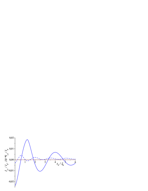
Figure 6: The dependence of the long-range amplitudes of the first $I_{1}$(solid line) and the second $I_{2}$ (dashed line) harmonics of the current–phase relation (14) on the shift of the central domain $z_{0}$. We have set $T=\mathrm{0.9}T_{c}$; $d=20\xi_{h}$; $d_{2}=2.5\xi_{h}$; $\alpha=\pi/2$. [ $I_{0}=(4eT_{c}N/\hbar)\left(\Delta/T_{c}\right)^{2}$ ].

Figure 6 shows the dependences of the function $T_{1}$ and $T_{2}$ on position of the central domain $z_{0}$ for different values of the rotation angle $\alpha$. We may see that the critical current is very sensitive to the position of the central domain and the first zero of $T_{1}$ occurs already at $z_{0}\simeq 0.5\xi_{h}$.

Certainly, the contribution of the second harmonic in the current–phase relation (14) is very small, because usually $|a_{2}|\ll|a_{1}|$, except very close to the $0-\pi$ transition ($T_{1}=0$). At this $0-\pi$ transition the contribution of the second harmonic $I_{2}$ becomes dominant. For all considered cases we obtained the positive amplitude of the second harmonic in the vicinity of these transitions, which means that they occur discontiguously by a jump between $0-$ and $\pi-$ phase states.

Supplementary Note 2: Arbitrary ferromagnetic barrier
The transfer–matrix formalism can be easily generalized for a layered ferromagnetic barrier with an arbitrary non-collinear distribution of the exchange field $\mathbf{h}$ which is described by the dependence $\alpha(z)$. Splitting the barrier on $N$ thin layers of the thickness $d_{i}=z_{i}-z_{i-1}\,(i=1\div N)$ one consider the exchange field to be constant inside each layer $i$. So, the transfer–matrix $\hat{T}_{\alpha_{i}}(d_{i},\theta)$ relates the components of the Green function $f(s)$ at the left ($s_{i-1}=z_{i-1}/\cos\theta$) and right ($s_{i}=z_{i}/\cos\theta$) boundaries of the $i-$layer:

$$\hat{f}(s_{i})=\hat{T}_{\alpha_{i}}(d_{i},\theta)\,\hat{f}(s_{i-1})\,.$$ (17)

Application of the transfer–matrix ”layer by layer” results in the following relation between the components of the Green function $f(0)$ and $f(s_{R})$ at the left and right superconducting electrodes, respectively:

$$\hat{f}(s_{R})=\hat{T}_{\alpha_{N}}(d_{N},\theta)\,\ldots\,\hat{T}_{\alpha_{2}}(d_{2},\theta)\,\hat{T}_{\alpha_{1}}(d_{1},\theta)\,\hat{f}(0)\,.$$ (18)

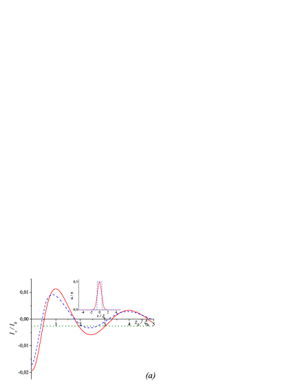
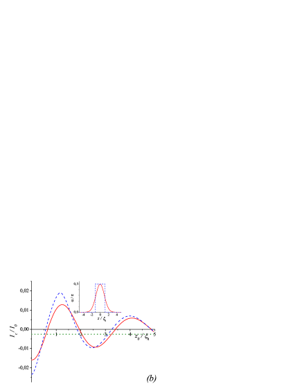
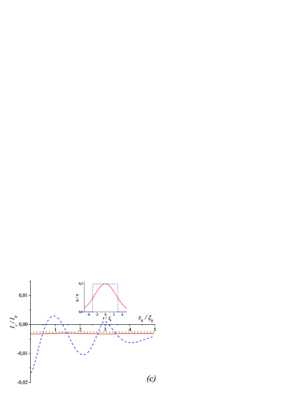
Figure 7: The dependence of the critical current $I_{c}=\mathrm{max}\{I_{1}+I_{2}\}$ on the shift $z_{0}$ of the $\mathrm{90^{o}}-$domain (19) ($\alpha=\pi/2$) for different values of the width of the transition region $w$ (solid red line): (a) $w=1$; (b) $w=2$; (c) $w=5$. The blue dashed line shows the dependence of the critical current $I_{c}$ on the shift $z_{0}$ of stepwise $\mathrm{90^{o}}-$domain for comparison. The dotted line shows the critical current $I_{c}$ in the absence of the domain ($\alpha=0$). Inset shows the coordinate dependence of the rotation angle $\alpha$ in the $\mathrm{90^{o}}-$domain (19)(red solid line) and the in the relevant stepwise domain (blue dashed line). We have set $d=20\xi_{h}$; $T=\mathrm{0.9}T_{c}$ [ $I_{0}=(4eT_{c}N/\hbar)\left(\Delta/T_{c}\right)^{2}$ ].

We apply the described transfer–matrix formalism to study the effect of smooth in the SFS constriction shown in Fig.2a of the Letter. As the dependence $\alpha(z)$ we use a draft model of $\mathrm{90^{o}}-$domain described by Gaussian funnction:

$$\alpha(z)=\frac{\pi}{2}\exp\left(-\frac{(z-z_{0})^{2}}{2w^{2}}\right)\,,$$ (19)

where $z_{0}$ is the shift of the domain with respect to the weak link center, and $w$ describes the width of the domain. Figure 7 shows the dependences of the critical current of the SFS junction on position $z_{0}$ of the $\mathrm{90^{o}}-$domain (19) for different values of the domain width $w$. We may see that the long–range effect seems to be completely disappeared if $w\gg\xi_{h}$ (see Fig. 7c), but it is quite robust for the domain width smaller than $2-3\xi_{h}$ and only weakly depends on the exact form of the transition region.

References

- 1 Barone, A. & Paterno, G. Physics and Application of the Josephson Effect (Wiley, New York, 1982).
- 2 Golubov, A. & Kupriyanov, M. & Ilichev, E. The current-phase relation in Josephson junctions. Rev. Mod. Phys. 76, 411–468 (2004).
- 3 Kaiser, U. & Schwarz, A. & Wiesendanger, R. Magnetic exchange force microscopy with atomic resolution. Rev. Mod. Phys. 76, 522–525 (2007).
- 4 Wiesendanger, R. Spin mapping at the nanoscale and atomic scale. Rev. Mod. Phys. 81, 1495 -1550 (2009).
- 5 Xiong, Y. M. & Stadler, S. & Adams, P. W. & Catelani, G. Spin-Resolved Tunneling Studies of the Exchange Field in EuS/Al Bilayers. Phys. Rev. Lett. 106, 247001-1 -247001-4 (2011).
- 6 Hamaya, K. et al. Kondo effect in a semiconductor quantum dot coupled to ferromagnetic electrodes. Appl. Phys. Lett. 91, 232105-1 -232105-3 (2007).
- 7 Pasupathy, A. N. et al. The Kondo Effect in the Presence of Ferromagnetism. Science 306, 86–89 (2004).
- 8 Demler, E. A. & Arnold, G. B. & Beasley, M. R. Superconducting proximity effects in magnetic metals. Phys. Rev. B 55, 15174 -15182 (1997).
- 9 Buzdin, A. I. Proximity effects in superconductor-ferromagnet heterostructures. Rev. Mod. Phys. 77, 935 -976 (2005).
- 10 Buzdin, A. I. & Bulaevskii, L. N. & Panyukov, S. V. Critical-current oscillations as a function of the exchange field and thickness of the ferromagnetic metal (F) in an S-F-S Josephson junction. Pis’ma Zh. Eksp. Teor. Fiz. 35, 147- 148 (1982)[JETP Lett. 35, 178 -180 (1982)].
- 11 Ryazanov, V. V. et al. Coupling of Two Superconductors through a Ferromagnet: Evidence for a Junction. Phys. Rev. Lett. 86, 2427 -2430 (2001).
- 12 Oboznov, V. A. et al. Thickness Dependence of the Josephson Ground States of Superconductor-Ferromagnet-Superconductor Junctions. Phys. Rev. Lett. 96, 197003-1 -197003-4 (2006).
- 13 Blanter, Ya. M. & Hekking, F. W. J. Supercurrent in long SFFS junctions with antiparallel domain configuration. Phys. Rev. B 69, 024525-1 -024525-4 (2004).
- 14 Buzdin, A. I. & Melnikov, A. S. & Pugach, N. G. Domain walls and long-range triplet correlations in SFS Josephson junctions. Phys. Rev. B 83, 144515-1 -144515-8 (2011).
- 15 Melnikov, A. S. & Samokhvalov, A. V. & Kuznetsova, S. M. & Buzdin, A. I. Interference Phenomena and Long-Range Proximity Effect in Clean Superconductor-Ferromagnet Systems. Phys. Rev. Lett. 109, 237006-1 -237006-5 (2012).
- 16 Bergeret, F. S. & Volkov, A. F. & Efetov, K. B. Long-Range Proximity Effects in Superconductor-Ferromagnet Structures. Phys. Rev. Lett. 86, 4096 -4099 (2001).
- 17 Kadigrobov, A. & Shekhter, R. I. & Jonson, M. Quantum spin fluctuations as a source of long–range proximity effects in diffusive ferromagnet-superconductor structures. Europhys. Lett. 54, 394 -400 (2001).
- 18 M. Houzet, M. & Buzdin, A. I. Long range triplet Josephson effect through a ferromagnetic trilayer. Phys. Rev. B 76, 060504-1 -060504-4 (2007).
- 19 Alidoust, M. & Linder, J. & Rashedi, G. & Yokoyama, T. & Sudbo, A. Spin-polarized Josephson current in superconductor/ferromagnet/superconductor junctions with inhomogeneous magnetization. Phys. Rev. B 81, 014512-1 -014512-9 (2010).
- 20 Volkov, A. F. & Efetov, K. B. Odd spin-triplet superconductivity in a multilayered superconductor-ferromagnet Josephson junction. Phys. Rev. B 81, 144522-1 -144522-13 (2010).
- 21 Robinson, J. W. A. & Witt, J. D. S. & Blamire, M. G. Controlled Injection of Spin-Triplet Supercurrents into a Strong Ferromagnet. Science 329, 59–61 (2010).
- 22 Khaire, T. S. & Khasawneh, M. A. & Pratt,Jr., W. P. & Birge, N. O. Observation of Spin-Triplet Superconductivity in Co-Based Josephson Junctions. Phys. Rev. Lett. 104, 137002-1 -137002-4 (2010).
- 23 Eilenberger, G. Transformation of Gorkov s equation for type II superconductors into transport-like equations. Z. f. Physik 214, 195 -213 (1968).
- 24 Champel, T. & Löfwander, T. & Eschrig, M. 0- Transitions in a Superconductor/Chiral Ferromagnet/Superconductor Junction Induced by a Homogeneous Cycloidal Spiral. Phys. Rev. Lett. 100, 077003-1 -077003-4 (2008).
- 25 Buzdin, A. I. Direct Coupling Between Magnetism and Superconducting Current in the Josephson Junction. Phys. Rev. Lett. 101, 107005-1 -107005-4 (2008).
- 26 Konschelle, F. & Buzdin, A. I. Magnetic Moment Manipulation by a Josephson Current. Phys. Rev. Lett. 101, 017001-1 -017001-4 (2009).
- 27 Grushina, A. L. & Dong-Keun Ki & Morpurgo, A. F. A ballistic pn junction in suspended graphene with split bottom gates. Appl. Phys. Lett. 102, 223102-1 -223102-4 (2013).
- 28 Biercuk, M. J. & Ilani, S. & Marcus, C. M. & McEuen, P. L. Carbon Nanotubes, A.Jorio, G.Dresselhaus and M.S.Dresselhaus, Eds., in. Topics Appl.Physics, 111 (Springer Verlag, Berlin Heidelberg, 2008).
- 29 Candini, A. et al. Graphene Spintronic Devices with Molecular Nanomagnets. Nano Letters 11, 2634 -2639 (2011).
- 30 Li, C. et al. Unipolar supercurrent through graphene grafted with Pt-porphyrins: signature of gate-tunable magnetism. arXiv: 1304.7089 v1, 1 -5 (2013).
- 31 Mourik, V. et al. Signatures of Majorana Fermions in Hybrid Superconductor-Semiconductor Nanowire Devices. Science 336, 1003–1007 (2012).
- 32 Haugen, H. & Huertas-Hernando, D. & Brataas, A. Spin transport in proximity-induced ferromagnetic graphene. Phys. Rev. B 77, 115406-1 -115406-8 (2008).
- 33 Semenov, Y. G. & Kim, K. W. & Zavada, J. M. Spin field effect transistor with a graphene channel. Appl. Phys. Lett. 91, 153105-1 -153105-3 (2007).