Deterministic polarization entanglement purification using time-bin entanglement

Abstract

We present a deterministic entanglement purification protocol (EPP) working for currently available experiment technique. In this protocol, we resort to the robust time-bin entanglement to purify the polarization entanglement determinately, which is quite different from the previous EPPs. After purification, one can obtain a completely pure maximally entangled pair with the success probability of 100%, in principle. As the maximal polarization entanglement is of vice importance in long-distance quantum communication, this protocol may have a wide application.

I Introduction

The distribution of entanglement states between long distant locations is essential for quantum communication computation1 ; computation2 ; teleportation . For instance, in order to achieve the faithful teleportation of unknown quantum states teleportation ; cteleportation , or quantum cryptograph Ekert91 ; BBM92 ; rmp , people first need to set up a quantum channel with maximally entangled state. Unfortunately, the source of entanglement is usually fragile. In a practical transmission, the interaction between a quantum entanglement system and the innocent noise of quantum channel always exists, which will make the maximally entangled state degrade and become a mixed state. A degraded quantum channel will make the fidelity of the teleportation degraded, and the key in the quantum cryptograph insecure. Therefore, before performing the quantum communication, they should recover the degraded entangled states into the maximally entangled states.

Entanglement purification is the method to obtain the maximally entangled states from the less-entangled ones. It has been widely used in quantum repeaters repeater ; DLCZ ; zhao ; chen ; Simon1 . The first entanglement purification protocol (EPP) was proposed by Bennett et al. in 1996 Bennett1 . It was used to purify the Werner state werner with quantum logical gate, i.e. controlled-NOT (CNOT) gate. This protocol was developed by Deustch et al. with similar quantum logical operations, subsequently Deutsch . The entanglement purification for multiparticle and high dimension system have also been proposed Murao ; Horodecki ; Yong . However, the CNOT gates or similar logical operations are very difficult to implement in current experiment.

On one hand, in long-distance quantum communication, photon encoded in the polarization degree of freedom is a best qubit system for its simple manipulation and fast transmission. In 2001, Pan et al. proposed an EPP with linear optics Pan1 . They used two polarization beam splitters (PBSs) to substitute the CNOT gates to complete the parity-check measurement which made the EPP can be easily realized in experiment. Subsequently, they have demonstrated entanglement purification for general mixed states of polarization-entangled photons in 2003 Pan2 . Later, some other EPPs were proposed, such as the EPP based on the cross-Kerr nonlinearity shengpra , the EPPs for single-photon entanglement sangouard , quantum-dot and microcavity system wangc2 ; wangc3 , and so on wangc1 ; dengfuguo2 ; peter1 ; peter2 ; hyperpurification ; hybirdpurification . These EPPs described above are all based on the frame of CNOT gates or similar logical operations. They should sacrifice a large number of low quality mixed states to improve the fidelity of the mixed states.

On the other hand, there is another way to realize polarization entanglement purification. It uses the other degrees of freedom entanglement to purify the polarization entanglement. In 2002, Simon and Pan first used the spatial entanglement to purify polarization entanglement with linear optics Simon . However, their protocol can only correct the bit-flip error. In 2010, Sheng et al. proposed a deterministic EPP, resorting to both spatial and frequency entanglement shengpra3 . However, their protocol is based on the weak cross-Kerr nonlinearity. It makes this protocol hard to realize. There are other deterministic EPPs based on the spatial entanglement shengpra4 ; lixh ; dengfuguo . Unfortunately, the spatial entanglement has its inherent drawback for the relative phase is sensitive to the length fluctuation zhao ; chen . Though phase can be well controlled in the experiment, as pointed out by Simon and Pan, it is still unrealistic in a practical long-distance quantum communication Simon ; Pan2 . Actually, using entanglement in other degree of freedom, such as spatial entanglement to purify the polarization entanglement is essentially the entanglement transformation. The reason is that the entanglement purification is based on the local operation and classical communication (LOCC). It is well known that LOCC cannot create the entanglement. The key idea of such EPP is to transfer the robust entanglement to the fragile entanglement.

Interestingly, qubits encoded in the time-bin degree of freedom are particularly suitable for long-distance quantum communication and fundamental experiments. The preparation of time-bin entangled states timebin1 ; timebin2 ; timebin3 ; timebin4 , violation of Bell inequalities timebin5 ; timebin6 , quantum key distribution timebin7 , teleportation timebin8 were widely discussed. Moreover, Humphreys et al. discussed the linear optical quantum computation in a single spatial mode timebin9 . One of the good advantages of time-bin entanglement is that it is a robust form of optical quantum information, especially for transmission in optical fibers. In 2002, Thew et al. have experimental investigated the robust time-bin qubits for distributed quantum communication over 11 kmThew . In 2004, Marcikic et al. also reported the experimental distribution of time-bin entangled qubits over 50 km of optical fibers. They demonstrated the violation of the Clauser-Horne-Shimony-Holt Bell inequality by more than 15 standard deviations without removing the imperfect detectors Marcikic . Recently, Donohue et al. reported their experimental results about the tomographically complete set of time-bin qubit projective measurements and showed that the fidelity of operations is sufficiently high to violate the Clauser-Horne-Shimony-Holt-Bell inequality by more than 6 standard deviations timebin10 .

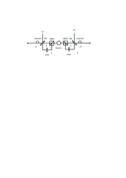
Figure 1: Schematic diagram showing the principle of converting the polarization entanglement to time-bin entanglement. The M-Z interferometer makes the state be in the different time bins. BS is the 50:50 beam splitter, and HWP is the half wave plate.

In this paper, we present a deterministic EPP resorting to the time-bin entanglement. We still use the concept of the entanglement purification to describe this protocol. Compared with the conventional EPPs, one can get a genuine pure entangled pair without consuming less-entangled pairs. Moreover, we do not require the initial state to be the hyperentanglement to complete the task. It will greatly release the complexity of the experiment. Moreover, the time-bin entanglement is more robust and can be well manipulated, which makes this EPP more useful in practical application.

II Deterministic EPP using time-bin entanglement

Now we start to explain this protocol by discussing a simple example. Interestingly, in this EPP, we do not require the polarization part to be entangled. Therefore, before the parties Alice and Bob share the polarization entangled pair, they first encode the initial pure polarization entanglement $|\Phi^{+}\rangle$ into the time-bin entanglement. As shown in Fig.1, after PBS1 and PBS2, the initial state $|\Phi^{+}\rangle$ evolves as

$$|\Phi^{+}\rangle_{AB} = \frac{1}{\sqrt{2}}(|H\rangle_{A}|H\rangle_{B}+|V\rangle_{A}|V\rangle_{B})$$

$$\longrightarrow \frac{1}{\sqrt{2}}(|H\rangle^{S}_{A}|H\rangle^{S}_{B}+|H\rangle^{L}_{A}|H\rangle^{L}_{B})$$

$$= |H\rangle_{A}|H\rangle_{B}\otimes\frac{1}{\sqrt{2}}(|S\rangle_{A}|S\rangle_{B}+|L\rangle_{A}|L\rangle_{B}).$$

The subscripts A and B mean that the photons transmit to Alice and Bob, respectively. The superscript S and L denote the different time bins. The L is the long arm and the S is the short arm. $|H\rangle$ and $|V\rangle$ denote horizontal and vertical polarizations of the single photon, respectively. After the photons passing through two 50:50 beam splitters (BSs), the system becomes

$$|\Phi^{+}\rangle_{AB} = \frac{1}{2}|H\rangle_{a1}|H\rangle_{a2}\otimes\frac{1}{\sqrt{2}}(|S\rangle_{a1}|S\rangle_{a2}+|L\rangle_{a1}|L\rangle_{a2})$$

$$+ \frac{1}{2}|H\rangle_{a1}|H\rangle_{b2}\otimes\frac{1}{\sqrt{2}}(|S\rangle_{a1}|S\rangle_{b2}-|L\rangle_{a1}|L\rangle_{b2})$$

$$+ \frac{1}{2}|H\rangle_{a2}|H\rangle_{b1}\otimes\frac{1}{\sqrt{2}}(|S\rangle_{a2}|S\rangle_{b1}-|L\rangle_{a2}|L\rangle_{b1})$$

$$+ \frac{1}{2}|H\rangle_{b1}|H\rangle_{b2}\otimes\frac{1}{\sqrt{2}}(|S\rangle_{b1}|S\rangle_{b2}+|L\rangle_{b1}|L\rangle_{b2}).$$

The initial state will be in the different spatial modes with same probability of $\frac{1}{4}$. Now we only discuss the transmission in channel a1a2. The same way can be used to the states in the channel a1b2, a2b1 and b1b2. The initial state with $|H\rangle_{a1}|H\rangle_{a2}\otimes\frac{1}{\sqrt{2}}(|S\rangle_{a1}|S\rangle_{a2}+|L\rangle_{a1}|L\rangle_{a2})$ can be rewritten as

$$\rho=\rho_{P}\otimes\rho_{T}.$$ (3)

Here $\rho_{P}$ is the polarization part with $\rho_{P}=|HH\rangle\langle HH|$, and $\rho_{T}$ time-bin part with $\rho_{T}=|\Phi\rangle_{T}\langle\Phi|$. Here $|\Phi\rangle_{T}=\frac{1}{\sqrt{2}}(|S\rangle|S\rangle+|L\rangle|L\rangle)$. After transmitted in the noisy channel, the polarization freedom of the photons is incident to be influenced by the vibration, the thermal fluctuation, or the distort of the fiber. These effects will lead the polarization entanglement to be degraded, and make the pure state $\rho_{P}$ become a mixed state $\rho^{\prime}_{P}$, with

$$\rho^{\prime}_{P} = F|\Phi^{+}\rangle\langle\Phi^{+}|+a|\Phi^{-}\rangle\langle\Phi^{-}|$$ (4)

$$+ b|\Psi^{+}\rangle\langle\Psi^{+}|+c|\Psi^{-}\rangle\langle\Psi^{-}|.$$

Here $F+a+b+c=1$, and

$$|\Phi^{-}\rangle = \frac{1}{\sqrt{2}}(|H\rangle|H\rangle-|V\rangle|V\rangle),$$

$$|\Psi^{\pm}\rangle = \frac{1}{\sqrt{2}}(|H\rangle|V\rangle\pm|V\rangle|H\rangle).$$ (5)

Fortunately, the time-bin entanglement is more robust than the polarization entanglement. After the state passing through the noisy channel, the whole state becomes

$$\rho^{\prime}=\rho^{\prime}_{P}\otimes\rho_{T},$$ (6)

and arrives at the setup for purification, as shown in Fig. 2.

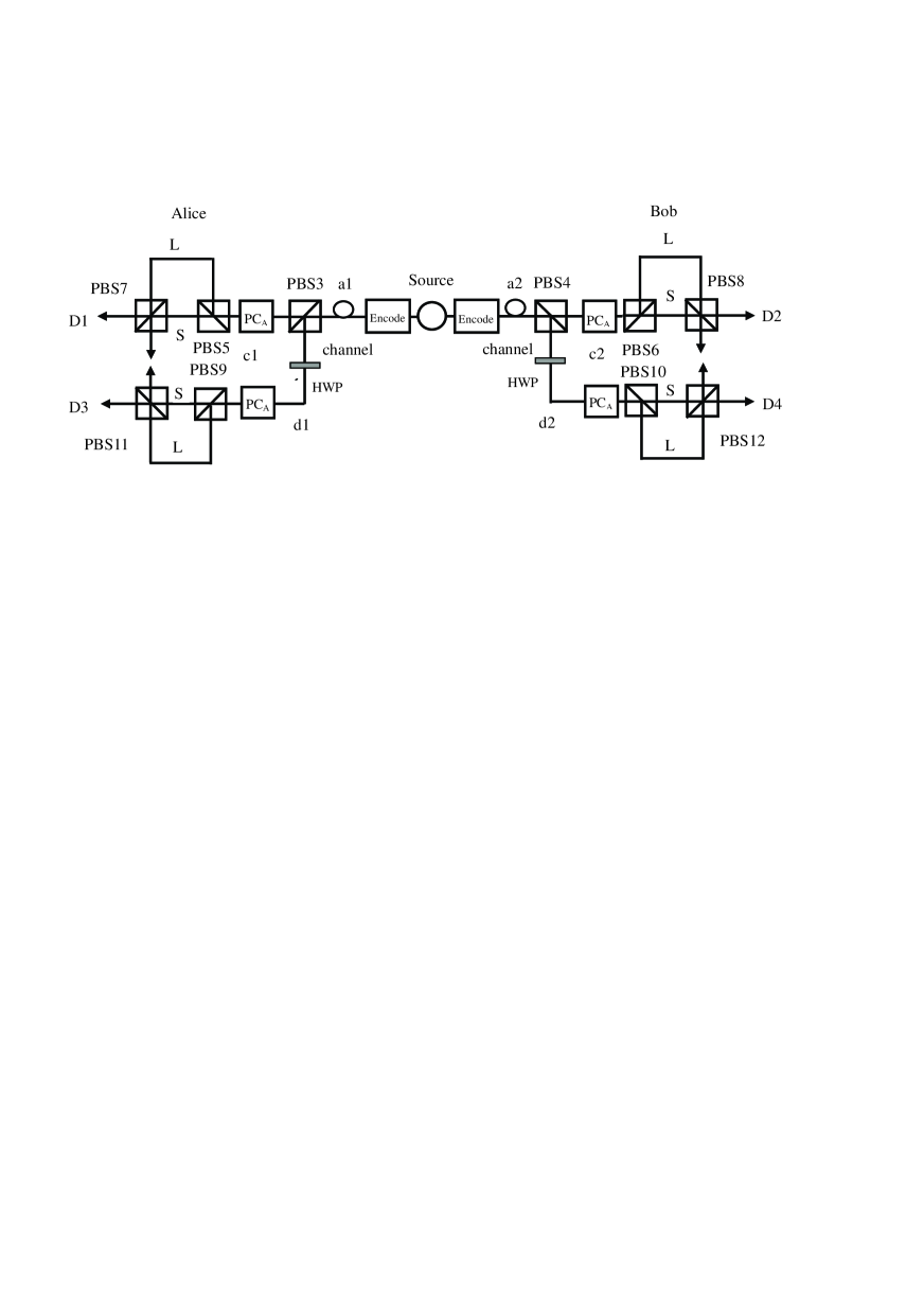
Figure 2: Schematic diagram showing the principle of purification. The PC_A is the Pockels cell. The mixed state of polarization can be divided into different spatial modes. This setup can purify the state which comes from a1a2 mode. The states in the other modes can also be purified by adding the similar setup. If the detectors D1D2, D1D4, D3D2 or D3D4 click, one can get the maximally entangled state $|\Phi^{+}\rangle$ determinately. The setup named ”Encode” is shown in Fig. 1.

The state $\rho^{\prime}$ can be described as: with the probability of $F$, state is in the $|\Phi^{+}\rangle|\Phi\rangle_{T}$. With the probability of $a$, state is in the $|\Phi^{-}\rangle|\Phi\rangle_{T}$. With the probability of $b$ and $c$, states are in $|\Psi^{+}\rangle|\Phi\rangle_{T}$ and $|\Psi^{-}\rangle|\Phi\rangle_{T}$, respectively.

We consider the case with $|\Phi^{+}\rangle|\Phi\rangle_{T}$. It can be written as $\frac{1}{2}(|H\rangle_{a1}|H\rangle_{a2}+|V\rangle_{a1}|V\rangle_{a2})(|S\rangle_{a1}|S\rangle_{a2}+|L\rangle_{a1}|L\rangle_{a2})$. We first discuss the item $|H\rangle_{a1}|H\rangle_{a2}\otimes\frac{1}{\sqrt{2}}(|S\rangle_{a1}|S\rangle_{a2}+|L\rangle_{a1}|L\rangle_{a2})$. After passing through the PBS3 and PBS4, the whole state evolves as

$$|H\rangle_{a1}|H\rangle_{a2}\otimes\frac{1}{\sqrt{2}}(|S\rangle_{a1}|S\rangle_{a2}+|L\rangle_{a1}|L\rangle_{a2})$$ (7)

$$\rightarrow |H\rangle_{c1}|H\rangle_{c2}\otimes\frac{1}{\sqrt{2}}(|S\rangle_{c1}|S\rangle_{c2}+|L\rangle_{c1}|L\rangle_{c2})$$

$$\rightarrow \frac{1}{\sqrt{2}}(|V\rangle_{c1}|V\rangle_{c2}\otimes|S\rangle_{c1}|S\rangle_{c2}+|H\rangle_{c1}|H\rangle_{c2}\otimes|L\rangle_{c1}|L\rangle_{c2})$$

$$= \frac{1}{\sqrt{2}}(|H\rangle^{L}_{c1}|H\rangle^{L}_{c2}+|V\rangle^{S}_{c1}|V\rangle^{S}_{c2}).$$

Here the PC_A is the Pockels cell pc . It precedes the polarization interferometers and coordinates by the time reference. It makes the PC_A work only at a time corresponding to the scheduled arrival of the early state of the photons, performing the transformation $|V^{S}\rangle\leftrightarrow|H^{S}\rangle$.

Finally, after the second Mach-Zehnder (M-Z) interferometer, the whole state becomes

$$\frac{1}{\sqrt{2}}(|H\rangle^{L}_{c1}|H\rangle^{L}_{c2}+|V\rangle^{S}_{c1}|V\rangle^{S}_{c2})$$ (8)

$$\rightarrow \frac{1}{\sqrt{2}}(|H\rangle^{LS}_{c1}|H\rangle^{LS}_{c2}+|V\rangle^{SL}_{c1}|V\rangle^{SL}_{c2})$$

$$= \frac{1}{\sqrt{2}}(|H\rangle_{D1}|H\rangle_{D2}+|V\rangle_{D1}|V\rangle_{D2}).$$

It is shown that they will obtain the maximally entangled state $|\Phi^{+}\rangle$ by detecting the photons with the single-photon detectors D$1$ and D$2$. The item $|V\rangle_{a1}|V\rangle_{a2}\otimes\frac{1}{\sqrt{2}}(|S\rangle_{a1}|S\rangle_{a2}+|L\rangle_{a1}|L\rangle_{a2})$ will be reelected by two PBSs and become $|H\rangle_{d1}|H\rangle_{d2}\otimes\frac{1}{\sqrt{2}}(|S\rangle_{d1}|S\rangle_{d2}+|L\rangle_{d1}|L\rangle_{d2})$. It can also become the maximally entangled state $|\Phi^{+}\rangle$ and finally be detected by D3 and D4.

The other states $|\Phi^{-}\rangle|\Phi\rangle_{T}$, $|\Psi^{\pm}\rangle|\Phi\rangle_{T}$ can evolve in the same way. For example, in the first item of $|\Phi^{-}\rangle|\Phi\rangle_{T}$, after the decoder setup, the item $|H\rangle_{a1}|V\rangle_{a2}\otimes\frac{1}{\sqrt{2}}(|S\rangle_{a1}|S\rangle_{a2}+|L\rangle_{a1}|L\rangle_{a2})$ becomes

$$|H\rangle_{a1}|V\rangle_{a2}\otimes\frac{1}{\sqrt{2}}(|S\rangle_{a1}|S\rangle_{a2}+|L\rangle_{a1}|L\rangle_{a2})$$ (9)

$$\rightarrow |H\rangle_{c1}|V\rangle_{d2}\otimes\frac{1}{\sqrt{2}}(|S\rangle_{c1}|S\rangle_{d2}+|L\rangle_{c1}|L\rangle_{d2})$$

$$\rightarrow |H\rangle_{c1}|H\rangle_{d2}\otimes\frac{1}{\sqrt{2}}(|S\rangle_{c1}|S\rangle_{d2}+|L\rangle_{c1}|L\rangle_{d2})$$

$$\rightarrow \frac{1}{\sqrt{2}}(|V\rangle_{c1}|V\rangle_{d2}\otimes|S\rangle_{c1}|S\rangle_{d2}$$

$$+ |H\rangle_{c1}|H\rangle_{d2}\otimes|L\rangle_{c1}|L\rangle_{d2})$$

$$= \frac{1}{\sqrt{2}}(|H\rangle^{L}_{c1}|H\rangle^{L}_{c2}+|V\rangle^{S}_{c1}|V\rangle^{S}_{c2})$$

$$\rightarrow \frac{1}{\sqrt{2}}(|H\rangle^{LS}_{c1}|H\rangle^{LS}_{d2}+|V\rangle^{SL}_{c1}|V\rangle^{SL}_{d2})$$

$$= \frac{1}{\sqrt{2}}(|H\rangle_{D1}|H\rangle_{D4}+|V\rangle_{D1}|V\rangle_{D4}).$$

The item $|V\rangle_{a1}|H\rangle_{a2}\otimes\frac{1}{\sqrt{2}}(|S\rangle_{a1}|S\rangle_{a2}+|L\rangle_{a1}|L\rangle_{a2})$ can also be used to obtain the maximally entangled state $|\Phi^{+}\rangle$ in the output modes D2D3, respectively. Here we only discuss the case that the state is in the mode of $a1a2$ with the probability of $\frac{1}{4}$. Other cases can be discussed in the same way. We should point out that, the state in the modes $a1b2$ and $a2b1$ can be purified to $\frac{1}{\sqrt{2}}(|HH\rangle-|VV\rangle)$.

III Discussion

So far, we have discussed the whole purification process. It is straightforward to extend this ECP to the case of multipartite state $\frac{1}{\sqrt{2}}(|HH\cdots H\rangle+|VV\cdots V\rangle)$. They first generate the state $|HH\cdots H\rangle\otimes\frac{1}{\sqrt{2}}(|SS\cdots S\rangle+|LL\cdots L\rangle)$. Then all the parties use the same setup shown in Fig. 2 to purify the polarization part. Finally they will obtain the maximally polarization entangled state with the same success probability of 100%. From above explanation, the realization of this EPP is essentially based on the robust time-bin entanglement. Several experiments described above showed that it is indeed robust for transmission in optical fiber. Actually, photons have the same transmission speed in the optical channel. The state $\frac{1}{\sqrt{2}}(|S\rangle|L\rangle+|L\rangle|S\rangle)$ comes from a bit-flip error never occur. On the other hand, the phase-flip error also does not exist. In the practical transmission, the phase-flip error mainly comes from the fluctuation of the path length. For example, in the DLCZ protocol for quantum repeaters, the single-photon entanglement is in the form of $\frac{1}{\sqrt{2}}(|01\rangle+e^{i\theta_{AB}}|10\rangle)$DLCZ . The phase $\theta_{AB}=\theta_{A}-\theta_{B}$ denotes the difference of the phase shifts in the left and the right sides of channelSimon1 ; sangouard . Here, path length fluctuations do not lead to the phase flip. Suppose a phase fluctuation occurs, it will make the two photons in the $|SS\rangle$ time-bin become $|S\rangle\otimes e^{i\theta}|S\rangle$, the same effect will be on the later time-bin state, which make $|LL\rangle\rightarrow|L\rangle\otimes e^{i\theta}|L\rangle$. The phase $\theta$ will become the global phase for the whole state and can be omitted. Thus, the state such as $\frac{1}{\sqrt{2}}(|SS\rangle-|LL\rangle)$ does not appear.

Local operations and classical communication cannot increase entanglement. The entanglement purification can be regarded as the transformation of the entanglement. In the previous protocol, they need two pairs of less-entangled state in each purification process, which means that the entanglement is transformed from the target pair to the source pair. It can be considered as the transformation between the same kind of degree of freedom. Surprisingly, Simon and Pan first pointed out that the entanglement purification can be happened in different degree of freedom Simon . Using the entanglement encoded in other degrees of freedom provides us a good way to perform the purification. Interestingly, one of the significant features of these kinds of EPPs is that it does not require the initial polarization part of the state to be entangled. It makes these kinds of EPP more like the protocol of entanglement distribution distribution .

It is interesting to compare the present protocol with the performances of the previous EPPs. The present protocol has several advantages. First, only one pair of state is required, while in the conventional EPPs, they always need two pair of low quality states. Second, we can get a maximally entangled pair, and the other conventional EPPs only improve the quality of the mixed state. They should consume a large number of low quality mixed states to obtain a small number of high quality mixed states. Compared with the other deterministic EPPs, this protocol does not resort to the hyperentanglement. Moreover, the time-bin entanglement is more robust than the entanglement encoded in the other degrees of freedom, which makes this protocol extremely suitable in practical application.

IV Conclusion

In conclusion, we have presented a determinate purification protocol for polarization entanglement state. The success probability for this protocol is 100%, in principle. We do not need large pairs of less-entangled states. As the time-bin entanglement is robust than the entanglement encoded in other degrees of freedom, this EPP may have its practical application in current long-distance quantum communication.

V ACKNOWLEDGMENTS

This work is supported by the National Natural Science Foundation of China (Grant No. 11104159), the Natural Science Research Project of Universities of Jiangsu Province, China (Grant No. 13KJB140010), and the Priority Academic Development Program of Jiangsu Higher Education Institutions, China.

References

- (1) Divincenzo D P 1995 Science 270 255
- (2) Bennett C H and Divincenzo D P 2000 Nature 404 247
- (3) Bennett C H, Brassard G, Crepeau C, Jozsa R, Peres A and Wootters W K 1993 Phys. Rev. Lett. 70 1895
- (4) Karlsson A and Bourennane M 1998 Phys. Rev. A 58 4394
- (5) Ekert A K 1991 Phys. Rev. Lett. 67 661
- (6) Bennett C H, Brassard G and Mermin N D 1992 Phys. Rev. Lett. 68 557
- (7) Gisin N, Ribordy G, Tittel W and Zbinden H 2002 Rev. Mod. Phys. 74 145
- (8) Briegel H J, Dür W, Cirac J I and Zoller P 1998 Phys. Rev. Lett. 81 5932
- (9) Duan L M, Lukin M D, Cirac J T and Zoller P 2001 Nature 414 413
- (10) Zhao B, Chen Z B, Chen Y A, Schmiedmayer J and Pan J W 2007 Phys. Rev. Lett. 98 240502
- (11) Chen Z B, Zhao B, Chen Y A, Schmiedmayer J and Pan J W 2007 Phys. Rev. A 96 022309
- (12) Simon C, de Riedmatten H, Afzelius M, Sanguard N, Zbinden H and Gisin N 2007 Phys. Rev. Lett. 98 190503
- (13) Bennett C H, Brassard G, Popescu S, Schumacher B, Smolin J A and Wootters W K 1996 Phys. Rev. Lett. 76 722
- (14) Werner R F 1989 Phys. Rev. A 40 4277
- (15) Deutsch D, Ekert A, Jozsa R, Macchiavello C, Popescu S and Sanpera A 1996 Phys. Rev. Lett. 77 2818
- (16) Murao M, Plenio M B, Popescu S, Vedral V and Knight P L 1998 Phys. Rev. A 57 R4075
- (17) Horodecki M and Horodecki P 1999 Phys. Rev. A 59 4206
- (18) Cheong Y W, Lee S W, Lee J and Lee H W 2007 Phys. Rev. A 76 042314
- (19) Pan J W, Simon C, and Zellinger A 2001 Nature 410 1067
- (20) Pan J W, Gasparonl S, Ursin R, Weihs G and Zellinger A Nature 2003 423 417
- (21) Sheng Y B, Deng F G and Zhou H Y 2008 Phys. Rev. A 77 042308
- (22) Sangouard N, Simon C, Coudreau T and Gisin N 2009 Phys. Rev. A 78 050301(R)
- (23) Wang C, Zhang Y and Jin G S 2011 Phys. Rev. A 84 032307
- (24) Wang C, Zhang Y, and Zhang R 2011 Opt. Exp. 19 25685
- (25) Xiao L, Wang C, Zhang W, Huang Y D, Peng J D and Long G L 2008 Phys. Rev. A 77 042315
- (26) Deng F G 2011 Phys. Rev. A 84 052312
- (27) Gonta D and van Loock P 2011 Phys. Rev. A 84 042303
- (28) Gonta D and van Loock P 2012 Phys. Rev. A 86 052312
- (29) Ren B C and Deng F G 2013 Laser Phys. Lett. 10 115201
- (30) Sheng Y B, Zhou L and Long G L 2013 Phys. Rev. A 88 022302
- (31) Simon C and Pan J W 2002 Phys. Rev. Lett. 89 257901
- (32) Sheng Y B and Deng F G 2010 Phys. Rev. A 81 032307
- (33) Sheng Y B and Deng F G 2010 Phys. Rev. A 82 044305
- (34) Li X H 2010 Phys. Rev. A 82 044304
- (35) Deng F G 2011 Phys. Rev. A 83 062316
- (36) Brendel J, Gisin N, Tittel W and Zbinden H 1999 Phys. Rev. Lett. 82 2594
- (37) Simon C and Poizat J P 2005 Phys. Rev. Lett. 94 030502
- (38) Barreiro J, Langford N, Peters N and Kwiat P 2005 Phys. Rev. Lett. 95 060501
- (39) Zavatta A, D Angelo M, Parigi V and Bellini M 2006 Phys. Rev. Lett. 96 020502
- (40) Franson J 1989 Phys. Rev. Lett. 62 2205
- (41) Olislager L, Cussey J, Nguyen A T, Emplit P, Massar S, Merolla J M and Huy K P 2010 Phys. Rev. A 82 013804
- (42) Tittel W, Brendel J, Zbinden H and Gisin N 2000 Phys. Rev. Lett. 84 4737
- (43) Marcikic I, de Riedmatten H, Tittel W, Zbinden H and Gisin N 2003 Nature 421 509
- (44) Humphreys P C, Metcalf B J, Spring J B, Moore M, Jin X M, Barbieri M, Kolthammer W S and Walmsley I A 2013 Phys. Rev. Lett. 111 150501
- (45) Thew R T, Tanzilli S, Tittel W, Zbinden H and Gisin N 2002 Phys. Rev. A 66 062304
- (46) Marcikic I, de. Riedmatten H, Tittel W, Zbinden H and Gisin N 2004 Phys. Rev. Lett. 93 180502
- (47) Donohue J M, Agnew M, Lavoie J, and Resch K J 2013 Phys. Rev. Lett. 111, 153602
- (48) Kalamidas D, 2005 Phys. Lett. A 343, 331
- (49) Li X H, Deng F G and Zhou H Y 2007 Appl. Phys. Lett. 91 144101