Fermion condensate generates a new state of matter by making flat bands

Abstract

This short review paper devoted to 90th anniversary of S. T. Belyaev birthday. Belyaev’s ideas associated with the condensate state in Bose interacting systems have stimulated intensive studies of the possible manifestation of such a condensation in Fermi systems. In many Fermi systems and compounds at zero temperature a phase transition happens that leads to a quite specific state called fermion condensation. As a signal of such a fermion condensation quantum phase transition (FCQPT) serves unlimited increase of the effective mass of quasiparticles that determines the excitation spectrum and creates flat bands. We show that the class of Fermi liquids with the fermion condensate forms a new state of matter. We discuss the phase diagrams and the physical properties of systems located near that phase transition. A common and essential feature of such systems is quasiparticles different from those suggested by L. D. Landau, by crucial dependence of their effective mass on temperature, external magnetic field, pressure etc. It is demonstrated that a huge amount of experimental data collected on different compounds suggests that they, starting from some temperature and down, form the new state of matter, and are governed by the fermion condensation. Our discussion shows that the theory of fermion condensation develops completely good description of the NFL behavior of strongly correlated Fermi systems. Moreover, the fermion condensation can be considered as the universal reason for the NFL behavior observed in various HF metals, liquids, compounds with quantum spin liquids, and quasicrystals. We show that these systems exhibit universal scaling behavior of their thermodynamic properties. Therefore, the quantum critical physics of different strongly correlated compounds is universal, and emerges regardless of the underlying microscopic details of the compounds. This uniform behavior, governed by the universal quantum critical physics, allows us to view it as the main characteristic of the new state of matter.

1 Introduction

S. T. Belyaev’s contribution to theoretical physics is very impressive. In 1958 S. T. Belyaev has published his classical works on the theory of nonideal Bose-gas. In these works, S. T. Belyaev demonstrates that peculiarity of Bose systems comes from a microscopic number of particles in the condensed state with the momentum $p=0$ bel1 ; bel2 . To deal with such a system, he suggests splitting the system into two parts or subsystems, the condensate with $p=0$ and the rest with $p>0$. It turns out that it is the condensate that creates the ”flavor” of Bose liquid, generating its vivid properties. One may try to figure out if physics like that of Bose systems could be represented in Fermi systems. Belyaev’s daring ideas of the two macroscopic parts in Bose systems is adopted by a theory of fermion condensate that permits to construct the new class of strongly correlated Fermi liquids with the fermion condensate (FC) ks ; pr1 ; 4 ; vol ; volovik2 , which quasiparticle system is also composed of two parts: One of them is represented by FC located at the chemical potential $\mu$, and giving rise to the spiky density of states (DOS) like that with $p=0$ of Bose system. Figure 1, panel A, shows DOS of a Fermi liquid with FC located at the momentum $p_{i}<p<p_{f}$ and energy $\varepsilon=\mu$. In contrast to the condensate of a Bose system occupying the $p=0$ state, quasiparticles of FC with the energy $\varepsilon=\mu$ must be spread out over the interval $p_{i}<p<p_{f}$.

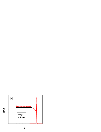
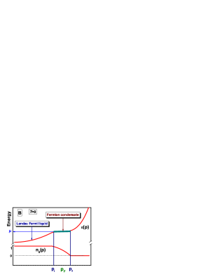
Figure 1: (Color online). Panel A, Schematic plot of the density of states (DOS) of quasiparticles versus energy $E$ at the momentum $p_{1}<p<p_{f}$ of a Fermi liquid with FC. Panel B, Schematic plot of two-component Fermi liquid at $T=0$ with FC. The system is separated into two parts shown by the arrows: The first part is a Landau Fermi liquid with the quasiparticle distribution function $n_{0}(p<p_{i})=1$, and $n_{0}(p>p_{f})=0$; The second one is FC with $0<n_{0}(p_{i}<p<p_{f})<1$ and the single-particle spectrum $\varepsilon(p_{i}<p<p_{f})=\mu$. The Fermi momentum $p_{F}$ satisfies the condition $p_{i}<p_{F}<p_{f}$.

The quasiparticle distribution function $n(\bf p)$ of Fermi system with FC is determined by the ordinary equation for a minimum of the Landau functional $E$ ks ; pr1 ; 4 . In contrast to common functionals of the number density $x$ hwk ; wks , the Landau functional of the ground state energy $E$ becomes the exact functional of the occupation numbers $n$. In case of homogeneous system a common functional becomes a function of $x=\sum_{p}n({\bf p})$, while E remains a functional, $E=E(n({\bf p}))$ pr1 ; 4 ,

$$\frac{\delta E(n({\bf p}))}{\delta n({\bf p})}=\varepsilon({\bf p})=\mu;\,\,{\rm if:\,}0<n({\bf p})<1.$$ (1)

Equation (1) represents an ordinary one to search the minimum of functional $E$. In the case of Bose system the equation $\delta E/\delta n(p)=\mu$ describes a common instance. In the case of Fermi systems such an equation, generally speaking, were not correct. Thus, it is the binding constraint $0<n({\bf p})<1$, taking place over some region $p_{i}<p<p_{f}$, that makes Eq. (1) applicable for Fermi systems. Because of the binding constraint, Fermi quasiparticles in the region $p_{i}<p<p_{f}$ can behave as Bose one, occupying the same energy level $\varepsilon=\mu$, and Eq. (1) yields the quasiparticle distribution function $n_{0}({\bf p})$ that minimizes the ground-state energy $E$. A possible solution $n_{0}({\bf p})$ of Eq. (1) and the corresponding single-particle spectrum $\varepsilon({\bf p})$ are depicted in Fig. 1, panel B. As seen from the panel B, $n_{0}({\bf p})$ differs from the step function in the interval $p_{i}<p<p_{f}$, where $0<n_{0}({\bf p})<1$, and coincides with the step function outside this interval. Thus, the Fermi surface at $p=p_{F}$ transforms into the Fermi volume at $p_{i}\leq p\leq p_{f}$ suggesting that the band is absolutely “flat” within this interval, giving rise to the spiky DOS. The existence of such flat bands formed by inter-particle interaction has been predicted for the first time in Ref. ks . Quasiparticles with momenta within the interval $(p_{i}<p<p_{f})$ have the same single-particle energies equal to the chemical potential $\mu$ and form FC, while the distribution $n_{0}({\bf p})$ describes the new state of the Fermi liquid with FC, and the Fermi system is split up into to parts: a Landau Fermi liquid (LFL) and the FC part, as it is shown in Fig. 1, panel B ks ; pr1 ; vol ; volovik2 ; 4 .

In contrast to the Landau, marginal, or Luttinger Fermi liquids, which exhibit the same topological structure of the Green’s function, in systems with FC, where the Fermi surface spreads into the Fermi volume, the Green’s function belongs to a different topological class. The topological class of the Fermi liquid is characterized by the invariant vol ; volovik2

$$N=tr\oint_{C}\frac{dl}{2\pi i}G(i\omega,{\bf p})\partial_{l}G^{-1}(i\omega,{\bf p}),$$ (2)

where “tr” denotes the trace over the spin indices of the Green’s function and the integral is taken along an arbitrary contour $C$ encircling the singularity of the Green’s function. The invariant $N$ in (2) takes integer values even when the singularity is not of the pole type, cannot vary continuously, and is conserved in a transition from the Landau Fermi liquid to marginal liquids and under small perturbations of the Green’s function. As shown by Volovik vol ; volovik2 , the situation is quite different for systems with FC, where the invariant $N$ becomes a half-integer and the system with FC transforms into an entirely new class of Fermi liquids with its own topological structure.

In contrast to Bose liquid, which entropy $S\to 0$ at temperature $T\to 0$, a Fermi liquid with FC possesses finite entropy $S_{0}$ at zero temperature 4 ; aplh . Indeed, as it is seen from Fig. 1, panel B, at $T=0$, the ground state of a system with a flat band is degenerate, and the occupation numbers $n_{0}({\bf p})$ of single-particle states belonging to the flat band are continuous functions of momentum ${\bf p}$, in contrast to discrete standard LFL values 0 and 1. Such behavior of the occupation numbers leads to a $T$-independent entropy term $S_{0}=S(T\to 0,n=n_{0})$ with the entropy given by

$$S(n)=-\sum_{\,{\bf p}}[n({\bf p})\ln n({\bf p})+(1-n({\bf p}))\ln(1-n({\bf p}))].$$ (3)

Since the state of a system with FC is highly degenerate, FC serves as a stimulator of phase transitions that could lift the degeneracy of the spectrum and make $S_{0}$ vanish in accordance with the Nernst theorem. For instance, FC can excite the formation of spin density waves, antiferromagnetic state and ferromagnetic state etc., thus strongly stimulating the competition between phase transitions eliminating the degeneracy. The presence of FC facilitates a transition to the superconducting state, because the both phases have the same order parameter ks ; 4 . Thus, in contrast to Bose systems with Bose condensate, entropy of which at lowering temperatures $S\to 0$, the $S_{0}$ peculiarity of Fermi systems with FC incites to the emerging of great diversity of states. Being generated by the same driving motive - $S_{0}$ - these, as we shall see, exhibit a universal behavior, and form a new state of matter demonstrated by many compounds.

In this paper we briefly review the theory of FC that permits to describe a tremendously broad variety of experimental results in different systems. We assume that these systems are located near the fermion condensation quantum phase transition (FCQPT), leading to the emergence of FC 4 ; ks . The rest of the paper is organized as follows. In Section 2, we examine a scaling behavior of the effective mass and heavy fermion (HF) metals based on the extended quasiparticle paradigm that is employed to renovate the Landau quasiparticle paradigm. In Section 3, we construct phase diagrams of Fermi systems with FC, and compare these with the experimental ones, and show that FC leads to a new state of matter. In Section 4, we apply the FC theory to describe the thermodynamic properties of strongly correlated Fermi systems represented by compounds holding a quantum spin liquid. Section 5 is devoted to quasicrystals. Section 6 summaries the main results.

2 Extended quasiparticle paradigm

Upon using the Landau functional, one can obtain the well-known Landau equation for the effective mass 4 ; 1_1 ; 1_2 ; lanl

$$\frac{1}{M^{*}}=\frac{1}{M}+\int\frac{{\bf p}_{F}{\bf p_{1}}}{p_{F}^{3}}F({\bf p_{F}},{\bf p}_{1},n)\frac{\partial n(\bf p_{1})}{\partial{\bf p_{1}}}\frac{d{\bf p}_{1}}{(2\pi)^{3}}.$$ (4)

Here, $F$ is the Landau interaction. For simplicity, we omit the spin dependencies. To calculate $M^{*}$ as a function of $T$, we construct the free energy $F=E-TS$, where $S$ is given by (3). Minimizing $F$ with respect to $n({\bf p})$, we arrive at the Fermi-Dirac distribution

$$n_{\pm}({\bf p},T)=\left\{1+\exp\left[\frac{(\varepsilon({\bf p},T)\pm B\mu_{B}-\mu)}{T}\right]\right\}^{-1}.$$ (5)

Here $\mu$ is the chemical potential, $B$ is an external magnetic field, and $\mu_{B}$ is the Bohr magneton. The term $\pm B\mu_{B}$ entering the right hand side of Eq. (5) describes Zeeman splitting. Eq. (4) is exact, and allows us to calculate the behavior of $M^{*}$ which now becomes a function of temperature $T$, external magnetic field $B$, number density $x$ and pressure $P$, rather than a constant. It is this feature of $M^{*}$ that forms both the scaling and the non-Fermi liquid (NFL) behavior observed in measurements on strongly correlated Fermi systems 4 ; UBH ; UFN . In case of finite $M^{*}$ and at $T=0$ the distribution function $n({\bf p},T=0)$ becomes the theta-function $\theta(p_{F}-p)$, as it follows from (5), and Eq. (4) yields the well-known result

$$\frac{M^{*}}{M}=\frac{1}{1-F^{1}/3}.$$ (6)

where $F^{1}=N_{0}f^{1}$, $f^{1}(p_{F},p_{F})$ is the $p$-wave component of the Landau interaction, $M$ is the bare mass of particles of the liquid in question, and $N_{0}=Mp_{F}/(2\pi^{2})$ is the DOS of a free Fermi gas. Because $x=p_{F}^{3}/3\pi^{2}$ in the Landau Fermi-liquid theory, the Landau interaction can be written as $F^{1}(p_{F},p_{F})=F^{1}(x)$. At a certain critical point $x=x_{FC}$ the denominator $(1-F^{1}(x)/3)$ tends to zero, $(1-F^{1}(x)/3)\propto(x-x_{FC})+a(x-x_{FC})^{2}+...\to 0$, and we find that

$$\frac{M^{*}(x)}{M}\simeq a_{1}+\frac{a_{2}}{x-x_{FC}}.$$ (7)

where $a_{1}$ and $a_{2}$ are constants and $M^{*}(x\to x_{FC})\to\infty$. As a result, at $T\to 0$ and $x\to x_{FC}$ the system undergoes a quantum phase transition 4 ; UFN , represented by FCQPT. We note that the divergence of the effective mass given by Eq. (7) does preserve the Pomeranchuk stability conditions, for $F^{1}$ is positive pom ; noz . The behavior of $M^{*}(x)$ given by (7) is in good agreement with the results of experiments on ³He 8 . The divergence of the effective mass $M^{*}(x)$ observed in measurements on two-dimensional ³He 8 is illustrated in Fig. 2. It is seen that calculations based on (7) are in good agreement with the experimental data.

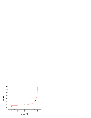
Figure 2: (Color online). The ratio $M^{*}/M$ in two-dimensional ³He as a function of the number density $x$ of the liquid, obtained from heat capacity and magnetization measurements. The experimental data are marked by black squares 8 , and the solid line represents the function given by Eq. (7).

It is instructive to briefly explore the behavior of $M^{*}$ in order to capture its universal behavior at FCQPT. Let us write the quasiparticle distribution function as $n_{1}({\bf p})=n({\bf p},T,B)-n({\bf p})$, with $n({\bf p})$ being the step function, and Eq. (4) then becomes

$$\frac{1}{M^{*}(T,B)}=\frac{1}{M^{*}}+\int\frac{{\bf p}_{F}{\bf p_{1}}}{p_{F}^{3}}F({\bf p_{F}},{\bf p}_{1})\frac{\partial n_{1}(p_{1},T,B)}{\partial p_{1}}\frac{d{\bf p}_{1}}{(2\pi)^{3}}.$$ (8)

At FCQPT, that is at $x\to x_{FC}$, the effective mass $M^{*}$ diverges and Eq. (8) becomes homogeneous, determining $M^{*}(T,B)$ as a universal function of temperature and magnetic field. The only role of $F$ is to drive the system to FCQPT and the solutions of Eq. (8) are represented by some universal function of variables $T$, $B$, $x$. In that case $M^{*}$ strongly depends on the same variables. In contrast to the Landau quasiparticle paradigm assuming the constancy of the effective mass, the extended quasiparticle paradigm is to be introduced 4 . The main point here is that the well-defined quasiparticles determine as before the thermodynamic, relaxation and transport properties of strongly correlated Fermi-systems, while $M^{*}$ becomes a function of $T$, $B$, $x$, etc.

2.1 Scaling behavior of both the effective mass and HF metals

A deeper insight into the behavior of $M^{*}(T,B)$ can be achieved using some ”internal” scales. Namely, near FCQPT the solutions of Eq. (8) exhibit a behavior so that $M^{*}(T,B)$ reaches its maximum value $M^{*}_{M}$ at some temperature $T_{M}\propto B$ 4 . It is convenient to introduce the internal scales $M^{*}_{M}$ and $T_{M}$ to measure the effective mass and temperature. Thus, we divide the effective mass $M^{*}$ and the temperature $T$ by the values, $M^{*}_{M}$ and $T_{M}$, respectively. This generates the normalized effective mass $M^{*}_{N}=M^{*}/M^{*}_{M}$ and the normalized temperature $T_{N}=T/T_{M}$.

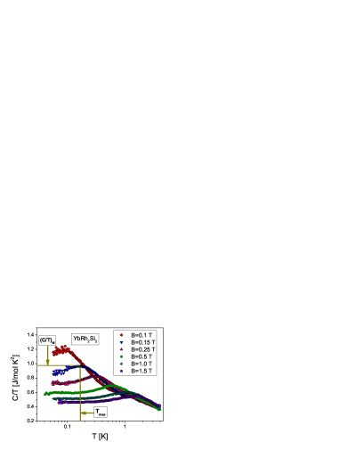
Figure 3: (Color online). Electronic specific heat of $\rm YbRh_{2}Si_{2}$, $C/T$, versus temperature $T$ as a function of magnetic field $B$ oesb shown in the legend. The illustrative values of $(C/T)_{M}\propto M^{*}_{M}$ and $T_{M}$ at $B=0.15$ T are shown.

As illustration to the above consideration, we analyze the specific heat $C/T\propto M^{*}$ of the HF metal $\rm YbRh_{2}Si_{2}$ oesb . Under the application of magnetic field $B$, the specific heat exhibits a behavior that is described by a function of both $T$ and $B$.

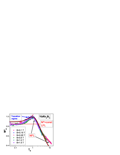
Figure 4: (Color online). The normalized effective mass $M^{*}_{N}$ versus normalized temperature $T_{N}$. $M^{*}_{N}$ is extracted from the measurements of the specific heat $C/T$ on $\rm YbRh_{2}Si_{2}$ in magnetic fields $B$ oesb listed in the legend. Constant effective mass $M^{*}_{L}$ inherent in a normal Landau Fermi liquid (LFL) is depicted by the solid line. The transition region is shown by the arrow and the NFL behavior is depicted by two arrows. Our calculation based on Eq. (4) is displayed by the solid curve.

As seen from Fig. 3, a maximum structure $(C/T)_{M}$ in $C/T\propto M^{*}_{M}$ at temperature $T_{M}$ appears under the application of magnetic field $B$. $T_{M}$ shifts to higher $T$ and $C/T\propto M^{*}_{M}$ diminishes as $B$ is increased. The value $C/T$ is saturated towards lower temperatures, decreasing at elevated magnetic field. To obtain the normalized effective mass $M^{*}_{N}$, we use $(C/T)_{M}$ and $T_{M}$ as ”internal” scales: The maximum structure $(C/T)_{M}$ was used to normalize $C/T$, and $T$ was normalized by $T_{M}$. In Fig. 4, the obtained $M^{*}_{N}=(C/T)/(C/T)_{M}=M^{*}/M^{*}_{M}$, as a function of normalized temperature $T_{N}=T/T_{M}$, is shown by geometrical figures. It is seen that the Landau Fermi liquid (LFL) state and NFL one are separated by the transition regime at which $M^{*}_{N}$ reaches its maximum value. Figure 4 reveals the scaling behavior of the normalized experimental curves - the curves at different magnetic fields $B$ merge into a single one in terms of the normalized variable $T/T_{M}$. Our calculations of the normalized effective mass $M^{*}_{N}(T_{N})$, shown by the solid line and based on Eq. (8), are in good agreement with the experimental facts 4 ; dft373 . Near FCQPT the normalized solution of Eq. (4) $M^{*}_{N}(T_{N})$ can be well approximated by a simple universal interpolating function 4 . The interpolation occurs between the LFL and NFL regimes and represents the universal scaling behavior of $M^{*}_{N}$ 4 ; dft373

$$M^{*}_{N}(T_{N})\approx c_{0}\frac{1+c_{1}T_{N}^{2}}{1+c_{2}T_{N}^{n}}.$$ (9)

Here, $c_{0}=(1+c_{2})/(1+c_{1})$, $c_{1}$, $c_{2}$ are fitting parameters; and the exponent $n=8/3$ if the Landau interaction is an analytical function otherwise $n=5/2$ 4 ; 14 . It follows from Eq. (9) that

$$T_{M}\simeq a_{1}\mu_{B}B,$$ (10)

where $a_{1}$ is a dimensionless factor.

Several remarks concerning the applicability of Eqs. (4) and (9) to systems with violated translational invariance are in order. We study the universal behavior of HF metals, quantum spin liquids, and quasicrystals at low temperatures using the model of a homogeneous HF liquid 4 . The model is applicable because we consider the scaling behavior exhibited by the thermodynamic properties of these materials at low temperatures, a behavior related to the scaling of quantities such as the effective mass $M^{*}$, the heat capacity $C/T\propto M^{*}$, the magnetic susceptibility $\chi\propto M^{*}$, etc. The behavior of $M^{*}_{N}(T_{N})$ that characterizes them are determined by momentum transfers that are small compared to momenta of the order of the reciprocal lattice length. The high momentum contributions can therefore be ignored by substituting the lattice for the jelly model. While the values of the scales like the maximum $M^{*}_{M}(B_{0})$ of the effective mass, measured at some field $B=B_{0}$, and $T_{M}$ at which $M^{*}_{M}$ takes place are determined by a wide range of momenta. Thus, these scales are controlled by the specific properties of the system under consideration. It follows from our consideration that the scaled thermodynamic properties of different strongly correlated Fermi systems can be described by universal function (9) determining $M^{*}_{N}(T_{N})$. It is seen from Fig. 4, and demonstrated by a huge amount of experimental data collected on strongly correlated Fermi systems that this observation is in good agreement with experimental facts 4 .

3 Phase diagrams of strongly correlated Fermi systems

At $T=0$, a quantum phase transition is driven by a nonthermal control parameter, e.g. the number density $x$, magnetic field $B$, pressure $P$. At the quantum critical point (QCP) related to FCQPT and taking place at $x=x_{FC}$, the effective mass $M^{*}$ diverges. We note that there are different kinds of instabilities of normal Fermi liquids connected with several perturbations of initial quasiparticle spectrum $\varepsilon(p)$ and occupation numbers $n(p)$, associated with the emergence of a multi-connected Fermi surface, see e.g. 4 ; khodb ; asp ; zvbld . Depending on the parameters and analytical properties of the Landau interaction, such instabilities lead to several possible types of restructuring of the initial Fermi liquid ground state. This restructuring generates topologically distinct phases. One of them is the FC, another one belongs to a class of topological phase transitions, where the sequence of rectangles $n(p)=0$ and $n(p)=1$ is realized at $T=0$. In fact, at elevated temperatures the systems located at these transitions exhibit behavior typical to those located at FCQPT 4 . Therefore, we do not consider the specific properties of these topological transitions, and focus on the behavior of systems located near FCQPT.

Beyond FCQPT, the system forms FC that leads to the emergence of a flat band protected by topological invariants vol ; volovik2 . The $T-x$ schematic phase diagram of the system which is driven to the FC state by variation of the number density $x$ is reported in Fig. 5. Upon approaching the critical density $x_{\rm FC}$ the system remains in the LFL region at sufficiently low temperatures, as it is shown by the shadow area. The temperature range of the shadow area shrinks as the system approaches QCP, and $M^{*}(x\to x_{FC})$ diverges as it follows from Eq. (7). At this QCP shown by the arrow in Fig. 5, the system demonstrates the NFL behavior down to the lowest temperatures. Beyond the critical point at finite temperatures the behavior remains the NFL, and is determined by the temperature-independent entropy $S_{0}$ 4 ; yakov . In that case at $T\to 0$, the system again demonstrates the NFL behavior, and approaches a quantum critical line (QCL) (shown by the vertical arrow and the dashed line in Fig. 5) rather than a quantum critical point. Upon reaching the quantum critical line from the above at $T\to 0$ the system undergoes the first order quantum phase transition, making $S_{0}$ vanish. As it is seen from Fig. 5, at rising temperatures the system located before QCP does not undergo a phase transition, and transits from the NFL behavior to the LFL one. At finite temperatures there is no boundary (or phase transition) between the states of the system located before or behind QCP, shown by the arrows. Therefore, at elevated temperatures the properties of systems with $x/x_{\rm FC}<1$ or with $x/x_{FC}>1$ become indistinguishable.

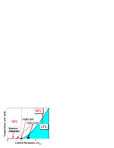
Figure 5: (Color online). Schematic $T-x$ phase diagram of system with FC. The number density $x$ is taken as the control parameter and depicted as $x/x_{FC}$. At $x/x_{FC}>1$ and sufficiently low temperatures, the system is in the LFL state as shown by the shadow area. This location of the system is depicted by both the solid square and the arrow. The vertical arrow illustrates the system moving in the LFL-NFL direction along $T$ at fixed control parameter. At $x/x_{FC}<1$ the system is shifted beyond the QCP, and is at the quantum critical line depicted by the dashed line and shown by the vertical arrow. This location of the system is shown by the short dash arrow. At any finite low temperatures $T>0$ the system possesses finite entropy $S_{0}$ and exhibits the NFL behavior.

As seen from Fig. 5, the location of the system is controlled by the number density $x$. At rising $x$, $x/x_{FC}>1$, the system is located before FCQPT, and demonstrates the LFL behavior at low temperatures. We speculate that such a state can be induced by the application of positive pressure, including positive chemical pressure. On the other hand, at diminishing $x$, $x/x_{FC}<1$, the system is shifted beyond FCQPT, and is at the quantum critical line depicted by the dashed line. In that case the system demonstrates the NFL behavior at any finite temperatures. We assume that such a state can be induced by the application of negative pressure, including negative chemical pressure. At low temperatures and above the critical line, the system has the finite entropy $S_{0}$ and its NFL state is strongly degenerate. The degeneracy stimulates the emergence of different phase transitions, lifting it and removing the entropy $S_{0}$. The NFL state can be captured by other states such as superconducting, for example, by the superconducting state (SC) in $\rm CeCoIn_{5}$, or by antiferromagnetic (AF) state, e.g. the AF in $\rm YbRh_{2}Si_{2}$ 4 ; dft373 ; yakov . The diversity of phase transitions occurring at low temperatures is one of the most spectacular features of the physics of many HF metals and strongly correlated compounds. Within the scenario of ordinary quantum phase transitions, it is hard to understand why these transitions are so different from one another and their critical temperatures are so extremely small. However, such diversity is endemic to systems with a FC, since the FC state must be altered as $T\to 0$, so that the excess entropy $S_{0}$ is shed before zero temperature is reached. At finite temperatures this takes place by means of some phase transitions which can compete, shedding the excess entropy 4 ; khodb .

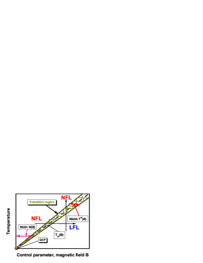
Figure 6: (Color online). Schematic $T-B$ phase diagram of HF liquid with magnetic field as the control parameter. The vertical and horizontal arrows show LFL-NFL and NFL-LFL transitions at fixed $B$ and $T$, respectively. At $B=0$ the system is in its NFL state, having a flat band, and demonstrates NFL behavior down to $T\to 0$. The hatched area separates the NFL phase and the weakly polarized LFL phase and represents the transition region. The dashed line in the hatched area represents the function $T_{M}(B)\simeq T^{*}_{FC}$ given by Eq. (10). The functions $W(B)\propto T$ and $T^{W}(B)\propto T$ shown by two-headed arrows define the width of the NFL state and the transition area, respectively. The QCP located at the origin and indicated by the arrow denotes the critical point at which the effective mass $M^{*}$ diverges and both $W(B)$ and $T^{W}(B)$ tend to zero.

The schematic $T-B$ phase diagram of a HF liquid is depicted in Fig. 6, with the magnetic field $B$ serving as the control parameter. At $B=0$, the HF liquid acquires a flat band corresponding to a strongly degenerate state. The NFL regime reigns at elevated temperatures and fixed magnetic field. With increasing $B$, the system is driven from the NFL region to the LFL domain. As shown in Fig. 6, the system moves from the NFL regime to the LFL regime along a horizontal arrow, and from the LFL to NFL along a vertical arrow. The magnetic-field-tuned QCP is indicated by the arrow and located at the origin of the phase diagram, since application of any magnetic field destroys the flat band and shifts the system into the LFL state 4 ; shag ; mig100 ; takah ; geg . The hatched area denoting the transition region separates the NFL state from the weakly polarized LFL state and contains the dashed line tracing the transition region, $T_{M}(B)\simeq T^{*}_{FC}$. Referring to Eq. (10), this line is defined by the function $T^{*}_{FC}\propto\mu_{B}B$, and the width $W(B)$ of the NFL state is seen to be proportional $T$. In the same way, it can be shown that the width $T^{W}(B)$ of the transition region is also proportional to $T$.

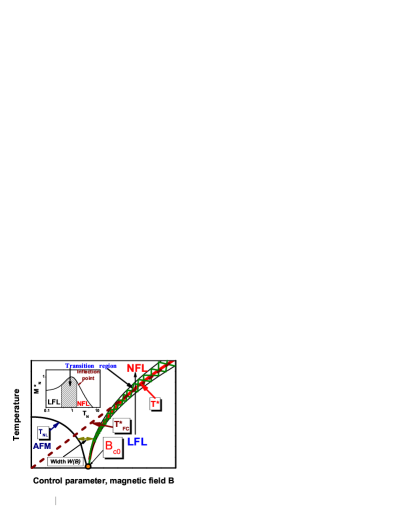
Figure 7: (Color online). Schematic $T-B$ phase diagram of a HF metal with magnetic field as the control parameter. The AF phase boundary line is shown by the arrow and depicted by the solid curve, representing the Néel temperature $T_{NL}$. The vertical and horizontal arrows show LFL-NFL and NFL-LFL transitions at fixed $B$ and $T$, respectively. The hatched area separates the NFL phase and the weakly polarized LFL phase and represents the transition area. The solid curve in the hatched area represents the transition temperature $T^{*}$. The solid short dash line $T^{*}_{FC}(B)\propto B\mu_{B}$ depicts the transition temperature provided that the AF state were absent. The functions $W(B)\propto T$ shown by two-headed arrows defines the total width of both the NFL state and the transition area. The inset shows a schematic plot of the normalized effective mass versus the normalized temperature. The transition regime, where $M^{*}_{N}$ reaches its maximum value at $T_{N}=T/T_{M}=1$, is shown as the hatched area in both the main panel and the inset. Arrows indicate the transition region and the inflection point $T_{inf}$ in the $M^{*}_{N}$ plot.

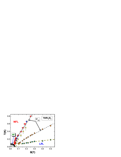
Figure 8: (Color online). Temperature versus magnetic field $T-B$ phase diagram for $\rm YbRh_{2}Si_{2}$. Solid circles represent the boundary between AF and NFL states. The curve is represented by the function $\sqrt{B-B_{c0}}$ 4 . The diamonds along the short-dash curve denote the transition area between the NFL and LFL regime steg1 ; geg . The short-dash line is approximated by $T^{*}_{FC}\propto B\mu_{B}$, see Fig. 7. Diamonds marking $T^{*}$ along this dash line signify the maxima $T_{M}$ of $C/T$ oesb shown in Fig. 3. The transition temperature $T^{*}$ as determined from magnetostriction (solid squares), longitudinal magnetoresistivity (triangles), and susceptibility (solid circles) steg1 . The solid line depicts the linear fit to $T^{*}$.

Now we construct the $T-B$ schematic phase diagram of a HF metal like $\rm YbRh_{2}Si_{2}$ shown in Fig. 7 4 ; jrho . We start with observing that Eq. (9) reveals the scaling behavior of the normalized effective mass $M^{*}_{N}(T_{N})$: Values of the effective mass $M^{*}(T,B)$ at different magnetic fields $B$ merge into a single mass value $M^{*}_{N}$ in terms of the normalized variable $T_{N}=T/T_{M}$. The inset in Fig. 7 demonstrates that scaling behavior of the normalized effective mass $M^{*}_{N}$ versus the normalized temperature $T_{N}$. The LFL phase prevails at $T\ll T_{M}$, followed by the $T^{-\beta}$ regime at $T\gtrsim T_{M}$, with $\beta=2/3$ or $\beta=1/2$ as it follows from Eq. (9). The latter phase is designated as NFL due to the strong dependence of the effective mass on temperature. The temperature region $T\simeq T_{M}$ encompasses the transition between the LFL regime with almost constant effective mass and the NFL behavior. Thus $T^{*}\sim T_{M}(B)$ identifies the transition region featuring a crossover between LFL and NFL regimes. The transition (crossover) temperature $T^{*}(B)$ is not actually the temperature of a phase transition. Its specification is necessarily ambiguous, depending as it does on the criteria invoked for determination of the crossover point. As usual, the temperature $T^{*}(B)$ is extracted from the field dependence of charge transport, for example from the resistivity $\rho(T)$ given by

$$\rho(T)=\rho_{0}+AT^{\alpha_{R}},$$ (11)

where $\rho_{0}$ is the residual resistivity and $A$ is a $T$-independent coefficient. The term $\rho_{0}$ is ordinarily attributed to impurity scattering. The LFL state is characterized by the $T^{\alpha_{R}}$ dependence of the resistivity with index $\alpha_{R}=2$. The crossover (through the transition regime shown as the hatched area in both Fig. 7 and its inset) takes place at temperatures where the resistance starts to deviate from LFL behavior, with the exponent $\alpha_{R}$ shifting from 2 into the range $1<\alpha_{R}<2$. When constructing the phase diagram depicted in Fig. 7, we assume that AF order wins the competition, destroying the $S_{0}$ term at low temperatures. At $B=B_{c0}$, the HF liquid acquires a flat band corresponding to a strongly degenerate state. Here, $B_{c0}$ is a critical magnetic field, such that at $T\to 0$ the application of magnetic field $B\gtrsim B_{c0}$ destroys the AF state restoring the paramagnetic state with the LFL behavior. In some cases as in the HF metal $\rm CeRu_{2}Si_{2}$, $B_{c0}=0$, see e.g. takah , while in $\rm YbRh_{2}Si_{2}$, $B_{c0}\simeq 0.06$ T geg . Obviously, $B_{c0}$ is defined by the specific system properties, therefore we consider it as a parameter. The NFL regime reigns at elevated temperatures and fixed magnetic field. With increasing $B$, the system is driven from the NFL region to the LFL domain. As shown in Figs. 6 and 7, the system moves from the NFL regime to the LFL regime along the corresponding arrows. The magnetic-field-tuned QCP is indicated by the arrow and located at $B=B_{c0}$. The hatched area denotes the transition region, and separates the NFL state from the weakly polarized LFL state. It contains both the dashed line tracing $T^{*}_{FC}(B)$ and the solid curve $T^{*}(B)$. Referring to Eq. (9), the latter is defined by the function $T^{*}\propto\mu_{B}B$ and merges with $T^{*}_{FC}(B)$ at relatively high temperatures, and $T^{*}\propto\mu_{B}(B-B_{c0})$ at lower $T\sim T_{NL}$, with $T_{NL}(B)$ being the Néel temperature. As seen from Eq. (9), both the width $W(B)$ of the NFL state and the width of the transition region are proportional $T$ jrho . The AF phase boundary line is shown by the arrow and depicted by the solid curve. As it was mentioned above, the dashed line $T^{*}_{FC}(B)\propto B\mu_{B}$ represents the transition temperature provided that the AF state were absent. In that case the FC state is destroyed by any weak magnetic field $B\to 0$ at $T\to 0$ and the dashed line $T^{*}_{FC}$ crosses the origin of coordinates, as it is displayed in Figs. 6 and 7. At $T\gtrsim T_{NL}(B=0)$ the transition temperature $T^{*}_{FC}(B)$ coincides with $T^{*}(B)$ shown by the solid curve, since the properties of the system are given by its local free energy, describing the paramagnetic state of the system. One might say that the system ”does not remember” the AF state, emerging at lower temperatures. This observation is in good agreement with experimental facts collected on the HF metal $\rm YbRh_{2}Si_{2}$. These experimental facts are summarized in the phase diagrams of Fig. 8: At relatively high temperatures $T\gtrsim T_{NF}(B=0)$ the transition temperature $T^{*}$, obtained in measurements on $\rm YbRh_{2}Si_{2}$ steg1 ; geg , is well approximated by the straight lines representing $T^{*}_{FC}$. It is seen from Fig. 8, that the slope of the short dash line (representing the maxima of the specific heat $C/T$) is different from the slope of the solid line (representing maxima of the susceptibility $\chi(T)$). Such a behavior is determined by the fact that the maxima of $C/T$ and $\chi(T)$ are given by the different relations, determining the inflection points of the entropy: $\partial^{2}S/\partial T^{2}=0$ and $\partial^{2}S/\partial B^{2}=0$, correspondingly. The theory of FC shows that the inflection points exist, provided that the system is located near FCQPT 4 ; jetp90 .

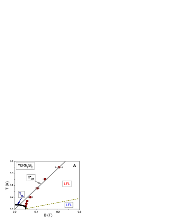
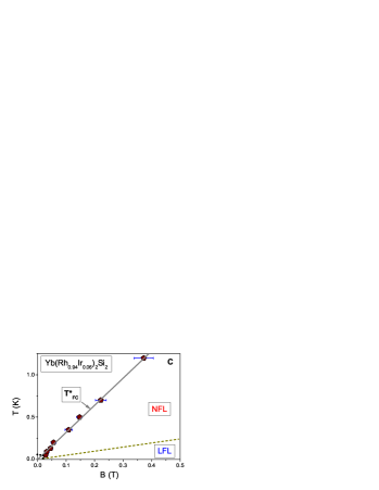
Figure 9: (Color online). $T-B$ phase diagrams for the three HF metals: $\rm YbRh_{2}Si_{2}$ (A); $\rm Yb(Rh_{0.93}Co_{0.07})_{2}Si_{2}$ (B); $\rm Yb(Rh_{0.94}Ir_{0.06})_{2}Si_{2}$ (C). In panels A and B, the AF phase boundaries pss are shown by the solid lines. In panel B, the diamonds depict the measurements pss . In panel C, the phase boundary of possible phase transition is shown by short dot curve. Pentagons correspond to the measurements of $T^{*}(B)$ on the HF metals extracted from the analysis of $\hat{\textbf{M}}$ as a function $B$ pss . The solid straight lines depict the transition temperature $T^{*}_{FC}(B)$. Dash lines schematically denote the boundary of the NFL and LFL regime.

Panels (A,B,C) of Fig. 9 are focused on the behavior of the transition temperature $T^{*}(B)$ extracted from measurements of kinks in $\hat{\textbf{M}}=\textbf{M}+(\textbf{dM}/dB)B$ as a function of $B$ pss , where M is the magnetization. Positions of the kinks is shown by pentagons in Fig. 9. It is seen from Fig. 9, panel A, that at $T\gtrsim T_{NL}(B=0)$, the transition temperature $T^{*}$ of $\rm YbRh_{2}Si_{2}$ is well approximated by the line $T^{*}_{FC}$. As mentioned above, upon using nonthermal tuning parameters like the number density $x$, the NFL behavior can be destroyed and the LFL one will be restored. In our simple model, the application of positive pressure $P$ makes $x$ grow shifting the system from FCQPT to the LFL state, as it is shown in Fig. 5, so that the electronic system of $\rm YbRh_{2}Si_{2}$ moves into the shadow area characterized by the LFL behavior at low temperatures. The new location of the system, represented by $\rm Yb(Rh_{0.93}Co_{0.07})_{2}Si_{2}$, is shown by the arrow pointing at the solid square. We note that the positive chemical pressure in the considered case is induced by $\rm Co$ substitution stegjap ; pss ; stegnat ; steg2 . As a result, the application of magnetic field $B\simeq B_{c0}$ does not drive the system to its FCQPT with the divergent effective mass because the QCP is already destroyed by the positive pressure, as it is shown in Fig. 9, panel B. Here $B_{c0}$ is the critical magnetic field that eliminates the corresponding AF order. At $B>B_{c0}$ and raising temperatures, the system, moving along the vertical arrow, transits from the LFL regime to the NFL one. At relatively high temperatures both $\rm YbRh_{2}Si_{2}$ and $\rm Yb(Rh_{0.93}Co_{0.07})_{2}Si_{2}$ are in their paramagnetic state. As a result, in that case $T^{*}$ is well approximated by the straight line $T^{*}_{FC}$. This observation is in accordance with experimental facts stegjap ; pss displayed in Fig. 9, panels A,B.

The system located above QCL exhibits the NFL behavior down to lowest temperatures unless it is captured by a phase transition. The behavior exhibiting by the system located above QCL is in accordance with the experimental observations that study the evolution of QCP in $\rm YbRh_{2}Si_{2}$ under the application of negative chemical pressure induced with $\rm Ir$ substitution stegjap ; pss ; stegnat ; steg2 . We assume a simple model that the application of negative pressure reduces $x$ and the electronic system of $\rm YbRh_{2}Si_{2}$ moves from QCP to a new position over QCL shown by the dash arrow in Fig. 5. Thus, the electronic system of $\rm Yb(Rh_{0.94}Ir_{0.06})_{2}Si_{2}$ is located at QCL and possesses a flat band, while the entropy includes $S_{0}$. We predict that at lowering temperatures, the electronic system of $\rm Yb(Rh_{0.94}Ir_{0.06})_{2}Si_{2}$ is captured by a phase transition, since the NFL state above QCL is strongly degenerate and the term $S_{0}$ should be eliminated. At diminishing temperatures, this degeneracy is to be removed by some phase transition which likely can be detected by the LFL state accompanying it. The tentative boundary line of that transition is shown by the short dot line in Fig. 9, panel C. It is also seen from Fig. 9, panel C, that at elevated temperatures $T^{*}$ is well approximated by the function $T^{*}_{FC}$.

Thus, at relatively high temperatures the transition temperature $T^{*}_{FC}(B)$, shown in Fig. 9, panels A, B, and C by the solid lines, coincides with $T^{*}(B)$ depicted by the pentagons. For, as it was discussed above, the local properties of the systems in question are given by their local free energy, formed by the NFL region related with FC, as it is displayed in Fig. 5.

To conclude this section, we have for the first time theoretically carried out a systematic study of the phase diagrams of strongly correlated Fermi systems, including HF metals like $\rm YbRh_{2}Si_{2}$, and considered the evolution of these diagrams in case of the application of negative/positive pressure. We have observed that at sufficiently high temperatures outside the AF phase the transition temperature $T^{*}(B)$ follows an almost linear B-dependence, and coincides with $T^{*}_{FC}(B)$, induced by the presence of FC. The obtained results are in good agreement with experimental facts stegjap ; pss ; stegnat ; steg2 .

As we shall show in Sections 4 and 5, the phase diagram 6 of HF liquid describes the corresponding phase diagrams of quantum spin liquids and quasicrystals as well, while the observed scaling behavior is described by Eq. (9). Thus, all these strongly correlated compounds exhibit the uniform behavior, and allow us to view that behavior as representing the main characteristic of the new state of matter.

4 Quantum spin liquid

The first experimental observation of quantum spin liquid (QSL) supporting exotic spin excitations - spinons - and carrying fractional quantum numbers in the herbertsmithite $\rm ZnCu_{3}(OH)_{6}Cl_{2}$ is reported in Ref. 15 . QSL can be viewed as an exotic quantum state composed of hypothetic particles such as fermionic spinons which carry spin $1/2$ and no charge. The herbertsmithite $\rm ZnCu_{3}(OH)_{6}Cl_{2}$ has been exposed as a $S=1/2$ Heisenberg antiferromagnet on a perfect kagome lattice, see Ref. 16 for a recent review. In $\rm ZnCu_{3}(OH)_{6}Cl_{2}$, the $\rm Cu^{2+}$ ions with $S=1/2$ form the triangular kagome lattice, and are separated by nonmagnetic intermediate layers of $\rm Zn$ and $\rm Cl$ atoms. The planes of the $\rm Cu^{2+}$ ions can be considered as two-dimensional (2D) layers with negligible magnetic interactions along the third dimension. A simple kagome lattice has a dispersionless topologically protected branch of the spectrum with zero excitation energy that is the flat band 17 ; 18 . In that case FCQPT can form a strongly correlated quantum spin liquid (SCQSL) composed of fermions with zero charge, $S=1/2$, and the effective mass $M^{*}_{\rm mag}$, occupying the corresponding Fermi sphere with the Fermi momentum $p_{F}$. A comparison of the QSL specific heat $C_{\rm mag}/T\propto M^{*}_{\rm mag}$ extracted from measurements on $\rm ZnCu_{3}(OH)_{6}Cl_{2}$ with $C/T$ of $\rm YbRh_{2}Si_{2}$ 19 ; 20 ; 21 is shown in Fig. 10. The striking feature of the specific heat behavior is the strong dependence on the magnetic field seen from the Figure. It is seen that both $C_{\rm mag}/T$ and $C/T$ exhibit the same qualitative behavior that allows us to view the herbertsmithite as insulator with QSL, and QSL itself as SCQSL 21 ; 22 ; 23 .

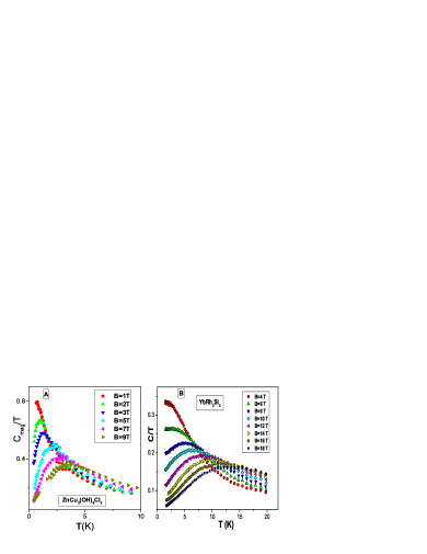
Figure 10: (Color online). Left panel: The specific heat $C_{\rm mag}/T$ of QSL is extracted from measurements of the specific heat on $\rm ZnCu_{3}(OH)_{6}Cl_{2}$ at different magnetic fields shown in the legend 19 ; 20 . Right panel reports the $T$-dependence of the electronic specific heat $C/T$ of $\rm YbRh_{2}Si_{2}$ at different magnetic fields 20 as shown in the legend.

The schematic $T-B$ phase diagram of $\rm ZnCu_{3}(OH)_{6}Cl_{2}$ is reported in Fig. 6. At $T=0$ and $B=0$ the system is near FCQPT without tuning. It can also be shifted from FCQPT by the application of magnetic field $B$. Magnetic field $B$ and temperature $T$ play the role of the control parameters, driving it from the NFL to LFL regions as shown by the vertical and horizontal arrows. At fixed $B$ and increasing $T$ the system transits along the vertical arrow from the LFL region to NFL one crossing the transition region. On the contrary, at fixed $T$ increasing $B$ drives the system along the horizontal arrow from the NFL region to LFL one. The inset to the phase diagram shown in Fig. 7 demonstrates the universal behavior of the normalized effective mass $M^{*}_{N}$ versus normalized temperature $T_{N}$ as given by Eq. (9). It follows from Eq. (9), and is seen from Fig. 6, that the both width $W$ of the NFL and the width $T^{W}$ of the transition region, shown by the arrows in Fig. 6, tend to zero at diminishing $T$ and $B$ since $W\propto T^{W}\propto T\propto B$.

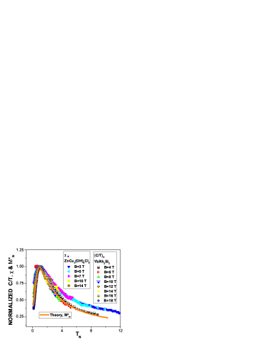
Figure 11: (Color online). The normalized effective mass $M^{*}_{N}$ extracted from measurements of susceptibility $\chi$ 24 on $\rm ZnCu_{3}(OH)_{6}Cl_{2}$ and $(C/T)$ on $\rm YbRh_{2}Si_{2}$ 20 . Our calculations of $M^{*}_{N}$ are shown by solid curve.

From Fig. 11 it is clearly seen that the data collected on both $\rm ZnCu_{3}(OH)_{6}Cl_{2}$ 24 and $\rm YbRh_{2}Si_{2}$ 20 merge into the same curve, obeying the scaling behavior. This demonstrates that the spin liquid of the herbertsmithite is close to FCQPT and behaves like HF liquid of $\rm YbRh_{2}Si_{2}$ in magnetic fields.

Figure 12 displays the normalized spin-lattice relaxation rates $(1/T_{1}T)_{N}$ at fixed temperature versus normalized magnetic field $B_{N}$. It is seen from Fig. 12, that the magnetic field $B$ progressively reduces $1/T_{1}T$, and the spin-lattice relaxation rate as a function of $B$ possesses an inflection point at some $B=B_{inf}$ shown by the arrow. To clarify the universal scaling behavior of QSL in the herbertsmithite and in HF metals, we normalize both the function $1/T_{1}T$ and the magnetic field. Namely, we normalize $(1/T_{1}T)$ by its value at the inflection point, and magnetic field is normalized by $B_{inf}$, $B_{N}=B/B_{inf}$. Since $(1/T_{1}T)_{N}=(M^{*}_{N})^{2}$ 4 ; t1rel , we expect that different strongly correlated Fermi systems located near FCQPT exhibit the same behavior of the normalized spin-lattice relaxation rate. It is seen from Fig. 12, that both the herbertsmithite $\rm ZnCu_{3}(OH)_{6}Cl_{2}$ imai and HF metal $\rm YbCu_{5-x}Au_{x}$ carr demonstrate similar behavior of the normalized spin-lattice relaxation rate. As seen from Fig. 12, at $B\leq B_{inf}$ (or $B_{N}\leq 1$), when the system in its NFL region, the normalized relaxation rate $(1/T_{1}T)_{N}$ depends weakly on the magnetic field, while at higher fields, as soon as the system enters the LFL region, $(1/T_{1}T)_{N}$ diminishes in agreement with both Eq. (9) and phase diagram 6,

$$(1/T_{1}T)_{N}=(M^{*}_{N})^{2}\propto B^{-4/3}$$ (12)

Thus, in accordance with the phase diagram shown in Fig. 6 and Eq. (12), we conclude that the application of magnetic field $B$ leads to crossover from the NFL to LFL behavior and to the significant reduction in the relaxation rate.

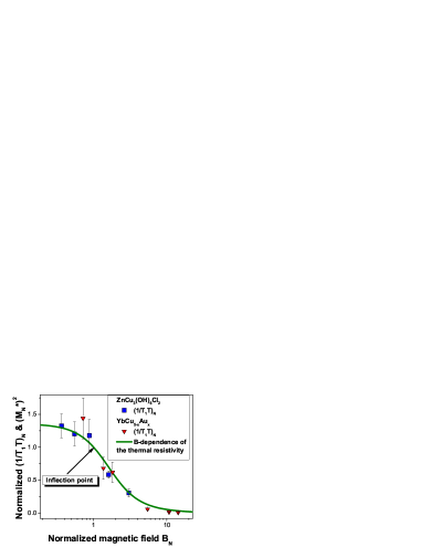
Figure 12: (Color online). The relaxation properties of the herbertsmithite versus those of HF metals. The normalized spin-lattice relaxation rate $(1/T_{1}T)_{N}$ at fixed temperature as a function of magnetic field: Solid squares correspond to data on $(1/T_{1}T)_{N}$ extracted from measurements on $\rm ZnCu_{3}(OH)_{6}Cl_{2}$ imai , while the solid triangles correspond to those extracted from measurements on $\rm YbCu_{5-x}Au_{x}$ with $x=0.4$ carr . The inflection point, representing the transition region, where the normalization is taken is shown by the arrow. Our calculations based on Eqs. (8) and Eq. (9) are depicted by the solid curve, tracing the scaling behavior of $(M^{*}_{N})^{2}$ and representing the $B$-dependence of the thermal resistivity $w$, see main text and Eq. (13).

As it was mentioned above, QSL plays a role of HF liquid framed into the insulating compound. Thus, we expect that QSL in the herbertsmithite behaves like the electronic liquid in HF metals if the charge of an electron were zero. In that case, the thermal resistivity $w$ of QSL is customarily related to the thermal conductivity $\kappa$

$$w=\frac{L_{0}T}{\kappa}=w_{0}+A_{w}T^{2}.$$ (13)

The resistivity $w$ behaves like the electrical resistivity $\rho=\rho_{0}+A_{\rho}T^{2}$ of the electronic liquid, since $A_{w}$ represents the contribution of spinon-spinon scattering to the thermal transport, being analogous to the contribution $A_{\rho}$ to the charge transport by electron-electron scattering. Here, $L_{0}$ is the Lorenz number, $\rho_{0}$ and $w_{0}$ are residual resistivity of electronic liquid and QSL, respectively, and the coefficients $A_{w}\propto(M^{*}_{\rm mag})^{2}$ and $A_{\rho}\propto(M^{*})^{2}$ 4 . Thus, in the LFL region the coefficient $A_{w}$ of the thermal resistivity of QSL under the application of magnetic fields at fixed temperature behaves like the spin-lattice relaxation rate shown in Fig. 12, $A_{w}(B)\propto 1/T_{1}T(B)\propto(M^{*}(B)_{\rm mag})^{2}$, while in the LFL region at fixed magnetic fields the thermal conductivity $\kappa$ is a linear function of temperature, $\kappa\propto T$.

Study of the thermal resistivity $w$ given by Eq. (13) allows one to reveal spinons as itinerant excitations. It is important that $w$ is not contaminated by contributions coming from localized excitations by impurity effects. The temperature dependence of thermal resistivity $w$ represented by the finite term $w_{0}$ directly shows that the behavior of QSL is similar to that of metals, and there is a finite residual term $\kappa/T$ in the zero-temperature limit of $\kappa$. The presence of this term immediately proves that there are gapless excitation associated with the property of normal metals, in which gapless electrons govern the heat transport. The finite $w_{0}$ means that in QSL both $k/T$ and $C_{mag}/T\propto M^{*}_{\rm mag}$ remain nonzero at $T\to 0$. Therefore, gapless spinons, forming the Fermi surface, govern the specific heat and the transport. Key information on the nature of spinons is further provided by the $B$-dependence of the coefficient $A_{w}$. The specific $B$-dependence of the resistivity $w(B)\propto(M^{*}_{\rm mag})^{2}$, shown in Fig. 12 and given by Eq. (12), would establish the behavior of QSL as SCQSL. We note that the heat transport is polluted by the phonon contribution. On the other hand, the phonon contribution is hardly influenced by the magnetic field $B$. Therefore, we expect the $B$-dependence of the heat conductivity to be governed by $A_{w}(B,T)$. Consider the approximate relation,

$$1 - \frac{A_{w}(B,T)}{A_{w}(0,T)}=1-\left(\frac{M^{*}(B,T)_{\rm mag}}{M^{*}(0,T)_{\rm mag}}\right)^{2}$$ (14)

$$\simeq a(T)\frac{\kappa(B,T)-\kappa(0,T)}{\kappa(0,T)}\equiv a(T)I(B,T),$$

where the coefficient $a(T)$ is $B$-independent. To derive (14), we employ Eq. (13), and obtain

$$\frac{\kappa}{L_{0}T}=\frac{1}{w_{0}+A_{w}T^{2}}+bT^{2}.$$ (15)

Here, the term $bT^{2}$ describes the phonon contribution to the heat transport. Upon carrying out simple algebra and assuming that $[1-A_{w}(B,T)/A_{w}(0,T)]\ll 1$, we arrive at Eq. (14). It is seen from Fig. 12, that the effective mass $M^{*}_{N}(B)\propto M^{*}_{\rm mag}(B)$ is a diminishing function of magnetic field $B$. Then, it follows from Eqs. (12) and (14) that the function $I(B,T)=[\kappa(B,T)-\kappa(0,T)]/\kappa(0,T)$ increases at elevated field $B$.

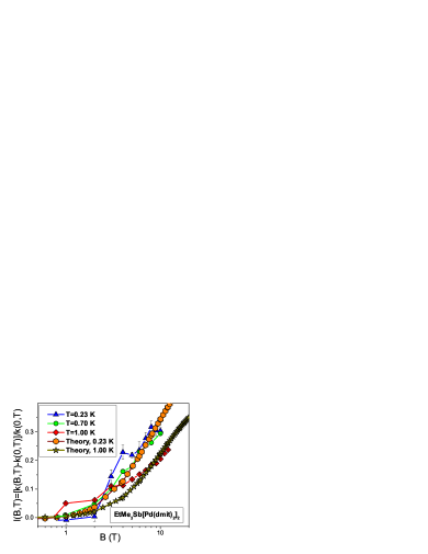
Figure 13: (Color online). Magnetic field $B$ dependence of the thermal conductivity $I(B,T)$ measured on the organic insulator $\rm EtMe{{}_{3}}Sb[Pd(dmit)_{2}]_{2}$ and standardized by the zero field value $\kappa$, $I(B,T)=[\kappa(B,T)-\kappa(B=0,T)]/\kappa(B=0,T)$ at temperatures shown in the legend scqsl ; chqs1 . Our calculations are based on Eq. (14) and shown by pentagons and stars.

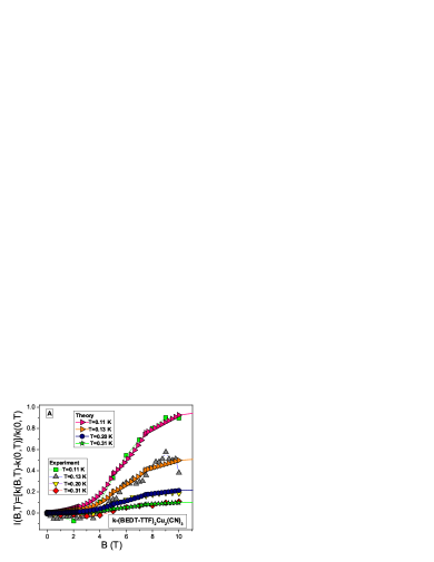
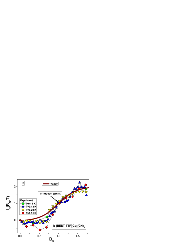
Figure 14: (Color online). Panel A: Magnetic field $B$ dependence of the thermal conductivity $I(B,T)$ measured on the organic insulator $\rm\kappa-(BEDT-TTF)_{2}Cu_{2}(CN)_{3}$ and standardized by the zero field value $\kappa$, $I(B,T)=[\kappa(B,T)-\kappa(B=0,T)]/\kappa(B=0,T)$ at temperatures shown in the legend chqs1 . Our calculations are based on Eq. (14) and shown by geometrical figures as it is displayed in the legend. Panel B: Normalized thermal conductivity $I_{N}(B_{N},T)$ as function of the normalized magnetic field $B_{N}$. The inflection point is shown by the arrow. Our calculations based on Eq. (14) are depicted by the solid curve.

Recent measurements of $\kappa(B)$ on the organic insulators $\rm EtMe{{}_{3}}Sb[Pd(dmit)_{2}]_{2}$ and $\rm\kappa-(BEDT-TTF)_{2}Cu_{2}(CN)_{3}$ scqsl ; chqs1 are displayed in Figs. 13 and 14. The measurements show that the heat is carried by phonons and QSL, for the heat conductivity is well fitted by $\kappa/T=a_{1}+a_{2}T^{2}$, where $a_{1}$ and $a_{2}$ are constants. The finite $a_{1}$ term implies that spinon excitations are gapless in $\rm EtMe{{}_{3}}Sb[Pd(dmit)_{2}]_{2}$, while in $\rm\kappa-BEDT-TTF)_{2}Cu_{2}(CN)_{3}$ gapless excitations are under debate chqs1 . A simple estimation indicates that the ballistic propagation of spinons seems to be realized in the case of $\rm EtMe{{}_{3}}Sb[Pd(dmit)_{2}]_{2}$ scqsl ; chqs1 . It is seen from Figs. 13 and 14, panel A, that the normalized data $I(B,T)=[\kappa(B,T)-\kappa(B=0,T)]/\kappa(B=0,T)$ demonstrate a strong $B$-dependence, namely the field dependence shows an increase of thermal conductivity for rising fields $B$. Such a behavior is in agreement with Eq. (12) and Fig. 12 which demonstrate that $(M^{*}(B)_{mag})^{2}$ is diminishing function of $B$. As a result, it follows from Eq. (14) that $I(B,T)$ is an increasing function of $B$. Our calculations based on Eqs. (14) and (8) are depicted by geometrical figures in Figs. 13 and 14, panel A. Since we cannot calculate the parameter $a(T)$ entering Eq. (14) we use it as a fitting parameter. Temperature $T$ was also used to fit the data at temperatures shown in the legend in Figs. 13 and 14. It is seen from Fig. 14, panel A, that $I(B,T)$ as a function of $B$ possesses an inflection point at some $B=B_{inf}$. To reveal the scaling behavior of QSL in $\rm\kappa-(BEDT-TTF)_{2}Cu_{2}(CN)_{3}$, we normalize both the function $I(B,T)$ and the magnetic field by their values at the inflection points, as it was done in the case of $(1/T_{1}T)$, see Fig. 12. In that case we get rid of the factor $a(T)$, entering Eq. (14), and our calculations do not have any fitting parameters. It is seen from Fig. 14, panel B, that the normalized $I_{N}(B_{N},T)$ exhibits the scaling behavior and becomes a function of a single variable $B_{N}$. Our calculations show that $I_{N}(B_{N},T)$ extracted from measurements on $\rm EtMe{{}_{3}}Sb[Pd(dmit)_{2}]_{2}$ exhibits the scaling behavior as well. It is seen from both Figs. 13 and 14, that our calculations are in good overall agreement with the experimental facts and there is no need to suppose the existence of additional magnetic excitations activated by the application of magnetic field in order to explain the growth of $I(B,T)$ at elevated $B$ scqsl ; chqs1 .

Important signature of electron liquid in HF metals is excitations — quasiparticles carrying electron quantum numbers and characterized by the effective mass $M^{*}_{\rm mag}$. Neutron scattering measurements of the dynamic spin susceptibility $\chi({\bf q},\omega,T)=\chi{{}^{\prime}}({\bf q},\omega,T)+i\chi{{}^{\prime\prime}}({\bf q},\omega,T)$ as a function of momentum $q$, frequency $\omega$ and and temperature $T$ play important role when identifying the properties of quasiparticles.

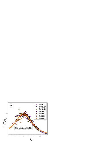
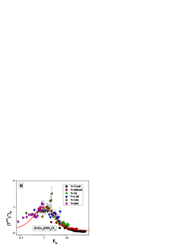
Figure 15: (Color online). Panel A: Normalized $(T^{2/3}\chi^{\prime\prime})_{N}$ plotted against the dimensionless variable $E_{N}$. The data are extracted from measurements on $\rm Ce_{0.925}La_{0.075}Ru_{2}Si_{2}$ 25 . Panel B: $(T^{2/3}\chi^{\prime\prime})_{N}$ versus $E_{N}$. The data are extracted from measurements on $\rm ZnCu_{3}(OH)_{6}Cl_{2}$ 24 . Our calculations are shown by the solid curves.

At low temperatures, such measurements allow one to reveal that quasiparticles excitations form a continuum, and populate an approximately flat band crossing the Fermi level. In that case the normalized susceptibility $(T^{2/3}\chi^{\prime\prime})_{N}$ exhibits a scaling behavior as a function of the dimensionless variable $E_{N}$ 23 . The panel A of Fig. 15 reports $(T^{2/3}\chi^{\prime\prime})_{N}$ extracted from measurements of the inelastic neutron scattering spectrum on the HF metal $\rm Ce_{0.925}La_{0.075}Ru_{2}Si_{2}$ 25 . The data $(T^{2/3}\chi^{\prime\prime})_{N}$ exhibit the scaling behavior over three orders of the variation of both the function and the variable. The scaled data obtained in measurements on a such quite different strongly correlated system as $\rm ZnCu_{3}(OH)_{6}Cl_{2}$ 24 are shown in the panel B. It is seen that our calculations shown by the solid curves are in good agreement with the experimental facts collected both on $\rm Ce_{0.925}La_{0.075}Ru_{2}Si_{2}$ and $\rm ZnCu_{3}(OH)_{6}Cl_{2}$ over almost three orders of the scaled variables jetp . Thus, the spin excitations in $\rm ZnCu_{3}(OH)_{6}Cl_{2}$ exhibit the same behavior as electron excitations of the HF metal $\rm Ce_{0.925}La_{0.075}Ru_{2}Si_{2}$, and, therefore form a continuum. This observation of the continuum is of great importance since it clearly reveals the presence of SCQSL in the herbertsmithite, as it was later confirmed by direct experimental observation 15 .

In this section, we have considered the non-Fermi liquid behavior and the scaling one of such strongly correlated Fermi systems as insulators $\rm ZnCu_{3}(OH)_{6}Cl_{2}$, $\rm EtMe{{}_{3}}Sb[Pd(dmit)_{2}]_{2}$, $\rm\kappa-(BEDT-TTF)_{2}Cu_{2}(CN)_{3}$, and HF metals $\rm Ce_{0.925}La_{0.075}Ru_{2}Si_{2}$, $\rm YbCu_{5-x}Au_{x}$, and $\rm YbRh_{2}Si_{2}$. We have shown that these are described within the frame of the theory of FC. Our calculations are in a good agreement with the experimental data, and allow us to identify the low-temperature behavior of $\rm ZnCu_{3}(OH)_{6}Cl_{2}$, $\rm\kappa-(BEDT-TTF)_{2}Cu_{2}(CN)_{3}$, and $\rm EtMe{{}_{3}}Sb[Pd(dmit)_{2}]_{2}$ as determined by SCQSL. The same behavior is observed in the heavy fermion metals. Thus, $\rm ZnCu_{3}(OH)_{6}Cl_{2}$, $\rm\kappa-BEDT-TTF)_{2}Cu_{2}(CN)_{3}$, and $\rm EtMe{{}_{3}}Sb[Pd(dmit)_{2}]_{2}$ can be viewed as a new type of strongly correlated electrical insulator that possesses properties of heavy-fermion metals with one exception: it resists the flow of electric charge, supporting the spin current formed by spinons.

5 Quasicrystals

New materials named quasicrystals (QCs) and characterized by noncrystallographic rotational symmetry and quasiperiodic translational properties have attracted scrutiny 26 . Study of quasicrystals may shed light on the most basic notions related to the quantum critical state observed in HF metals. Experimental measurements on the gold-aluminium-ytterbium quasicrystal $\rm Au_{51}Al_{34}Yb_{15}$ have revealed a quantum critical behavior with the unusual exponent $\beta\simeq 0.51$ defining the divergency of the magnetic susceptibility $\chi\propto T^{-\beta}$ at $T\to 0$ 27 . The measurements have also exposed that the observed NFL behavior transforms into the LFL one under the application of a tiny magnetic field $B$. All these facts challenge theory to explain a quantum criticality of the gold-aluminum-ytterbium QC. In case of QCs electrons occupy a new class of states denoted as ”critical states”, neither being extended nor localized. Associated with these critical states, characterized by an extremely degenerate confined wave function, are the so-called ”spiky” DOS 28 . These predicted DOS are corroborated by experiments revealing that single spectra of the local DOS demonstrate the spiky DOS 29 , which form flat bands 30 . As a result, we assume that the electronic system of some quasicrystals is located at FCQPT without tuning.

We now investigate the behavior of $\chi$ as a function of temperature at fixed magnetic fields. The effective mass $M^{*}(T,B)$ can be measured in experiments, for $M^{*}(T,B)\propto\chi$, where $\chi$ is the ac or dc magnetic susceptibility. If the corresponding measurements are carried out at fixed magnetic field $B$ then, as it follows from Eq. (9), $\chi$ reaches the maximum $\chi_{M}$ at some temperature $T_{M}$. Upon normalizing both $\chi$ and the specific heat $C/T$ by their peak values at each field $B$ and the corresponding temperatures by $T_{M}$, we observe from Eq. (9) that all the curves are to merge into a single one, thus demonstrating a scaling behavior typical for HF metals 4 . As seen from Fig. 16, $\chi_{N}$ extracted from measurements on $\rm Au_{51}Al_{34}Yb_{15}$ 27 shows the scaling behavior given by Eq. (9) and agrees well with our calculations shown by the solid curve over four orders of magnitude in the normalized temperature. It is also seen, that $\chi_{N}$ agrees well with the normalized $(C/T)_{N}$ extracted from measurements in magnetic fields on $\rm YbRh_{2}Si_{2}$ pikul . At $T_{N}>1$ the susceptibility $\chi_{N}$ exhibits the $T^{-\beta}$ regime, $\chi_{N}(T)\propto T^{-\beta}$, with $\beta=1/2$.

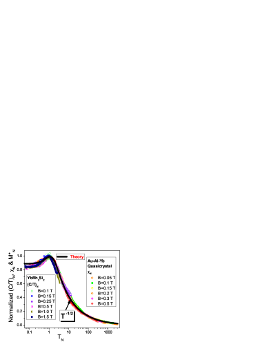
Figure 16: (Color online). The normalized specific heat $(C/T)_{N}$ and the normalized magnetic susceptibility $\chi_{N}$ extracted from measurements in magnetic fields $B$ on $\rm YbRh_{2}Si_{2}$ pikul and on $\rm Au_{51}Al_{34}Yb_{15}$ 27 , respectively. The corresponding magnetic fields are listed in the legends. The arrow shows the $T^{-1/2}$ regime taking place at $T_{N}>1$. Our calculations are depicted by the solid curve tracing the scaling behavior of $(C/T)_{N}=\chi_{N}=M^{*}_{N}$ given by Eq. (9).

The schematic phase diagram of the gold-aluminum-ytterbium QC $\rm Au_{51}Al_{34}Yb_{15}$ is reported in Fig. 6. The magnetic field $B$ plays the role of the control parameter, driving the system outwards FCQPT that occurs at $B=0$ and $T=0$ without tuning, since the QC critical state is formed by singular density of states 27 ; 28 ; 29 ; 30 . It follows from Eq. (9) and is seen from Fig. 6, that at fixed temperatures the increase of $B$ drives the system along the horizontal arrow from NFL state to LFL one. On the contrary, at fixed magnetic field and increasing temperatures the system transits along the vertical arrow from LFL state to NFL one. The $T^{-\beta}$ regime with $\beta=1/2$ is marked as NFL since contrary to the LFL case, where the effective mass is constant, the effective mass depends strongly on temperature. Thus, the temperatures $T^{*}_{FC}\simeq T_{M}$, shown by the arrow in Fig. 6, can be regarded as the transition regime between LFL and NFL states. It is seen, that the common width of the LFL region $W$ and the transition one $T^{W}$ is proportional to $T$. These theoretical results are in good agreement with the experimental facts 27 .

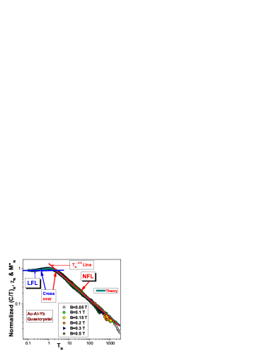
Figure 17: (Color online). Temperature dependence on the double logarithmic scale of the normalized effective mass $M^{*}_{N}$ versus normalized temperature $T_{N}$ extracted from measurements of the magnetic susceptibility $\chi$ on the quasicrystal $\rm Au_{51}Al_{35}Yb_{14}$ at different magnetic fields 27 shown in the legend. The LFL region and NFL one are shown by the solid and dashed arrows, respectively. The crossover region is depickted by two arrows. The solid line marked by the NFL displays $M^{*}_{N}\propto T_{N}^{-0.5}$ behavior.

In order to validate the phase diagram displayed in Fig. 6, we focus on the LFL, NFL and the transition LFL-NFL regions exhibited by the QC. To this end, we display in Fig. 17 the normalized $\chi_{N}$ on the double logarithm scale. As seen from Fig. 17, $\chi_{N}$ extracted from the measurements is not a constant, as would be for a LFL. The two regions (the LFL region and NFL one), separated by the transition region, as depicted by the hatched area in Fig. 6, are clearly seen in Fig. 17 illuminating good agreement between the theory and measurements. The straight lines in Fig. 17 outline both the LFL and NFL behaviors of $\chi_{N}\propto const$ and $\chi_{N}\propto T_{N}^{-1/2}$. These straight lines in Fig. 17 are in good agreement with the behavior of $M^{*}_{N}$ given by Eq. (9) with $n=5/2$. It is also seen from Fig. 17 that a tiny magnetic field of $B=0.05$ T destroys the NFL behavior hereby driving the system to the LFL region 14 . It is seen that our calculations shown by the solid curve are in good agreement with the experimental facts over four orders of magnitude in the normalized temperature.

As a result, we conclude that $\rm Au_{51}Al_{34}Yb_{15}$ quasicrystal exhibits the typical scaling behavior of its thermodynamic properties, and belongs to the famous family of HF metals, while the quantum critical physics of the quasicrystal is universal, and emerges regardless of the underlying microscopic details of the quasicrystal.

6 Summary

The condensate state in Bose interacting systems, introduced by S. T. Belyaev in his famous papers, forms the system’s properties. It turns out that the fermion condensate takes place in many compounds, and generates the non-Fermi liquid behavior by forming flat bands. We have for the first time theoretically carried out a systematic study of the phase diagrams of strongly correlated Fermi systems, including HF metals, insulators with strongly correlated quantum spin liquid, and quasicrystals, and have demonstrated that these diagram have universal features. The obtained results are in good agreement with experimental facts. We have shown both analytically and using arguments based entirely on the experimental grounds that the data collected on very different heavy-fermion compounds, such as HF metals, compounds with quantum spin liquid and quasicrystals, have a universal scaling behavior, and materials with strongly correlated fermions can unexpectedly have a uniform behavior in spite of their microscopic diversity. Thus, the quantum critical physics of different heavy-fermion compounds is universal, and emerges regardless of the underlying microscopic details of the compounds. This uniform behavior, induced by the universal quantum critical physics, allows us to view it as the main characteristic of the new state of matter. Our analysis of strongly correlated systems is in the context of salient experimental results, and our calculations of the non-Fermi liquid behavior are in good agreement with a broad variety of experimental facts. Our theoretical analysis of numerous experimental facts shows that the theory of fermion condensation develops completely good description of the NFL behavior of strongly correlated Fermi systems. Moreover, the fermion condensate can be considered as the universal reason for the NFL behavior observed in various HF metals, liquids, insulators with quantum spin liquids, and quasicrystals.

7 acknowledgement

This paper is written as invited review dedicated to 90th anniversary of S. T. Belyaev birthday.

KGP acknowledges funding from the Ural Branch of the Russian Academy of Sciences, basic research program no. 12-U-1-1010, the Presidium of the Russian Academy of Sciences, program 12-P1-1014, and RTP UrB RAS project P3.

References

- (1) S. T. Belyaev, Sov. Phys. JETP 34, 417 (1958).
- (2) S. T. Belyaev, Sov. Phys. JETP 34, 433 (1958).
- (3) V. A. Khodel and V. R. Shaginyan, JETP Lett. 51, 553 (1990).
- (4) V. A. Khodel, V. R. Shaginyan, and V. V. Khodel, Phys. Rep. 249, 1 (1994).
- (5) V. R. Shaginyan, M. Ya. Amusia, A. Z. Msezane, and K. G. Popov, Phys. Rep. 492, 31 (2010).
- (6) G. E. Volovik, JETP Lett. 53, 222 (1991).
- (7) G. E. Volovik, Springer Lecture Notes in Phys. 718, 31 (2007).
- (8) P. Hohenberg and W. Kohn, Phys. Rev. 136, B864 (1965).
- (9) W. Kohn and L. J. Sham, Phys. Rev. 140, A1133 (1965).
- (10) M. V. Zverev, V. A. Khodel, V. R. Shaginyan, and M. Baldo, JETP Lett. 65, 863 (1997).
- (11) L. D. Landau, Sov. Phys. JETP 5, 101 (1957).
- (12) L. D. Landau, Sov. Phys. JETP 8, 70 (1959).
- (13) E. M. Lifshitz and L. P. Pitaevskii, Statistical Physics, Pt. 2, Pergamon Press, Oxford, 1980.
- (14) V. R. Shaginyan, JETP Lett. 79, 286 (2004).
- (15) V. R. Shaginyan, M. Ya. Amusia, and K. G. Popov, Physics-Uspekhi 50, 563 (2007).
- (16) I. Ya. Pomeranchuk, Sov. Phys. JETP 8, 361 (1958).
- (17) P. Nozières, J. Phys. I France 2, 443 (1992).
- (18) A. Casey, H. Patel, J. Nyeki, B.P. Cowan, and J. Saunders, J. Low Temp. Phys. 113, 293 (1998).
- (19) N. Oeschler, S. Hartmann, A. P. Pikul, C. Krellner, C. Geibel, and F. Steglich, Physica B 403, 1254 (2008).
- (20) V. R. Shaginyan, M. Ya. Amusia, and K. G. Popov, Phys. Lett. A 373, 2281 (2009).
- (21) V. R. Shaginyan, A. Z. Msezane, K. G. Popov, G. S. Japaridze, and V. A. Khodel, Phys. Rev. B 87, 245122 (2013).
- (22) S. A. Artamonov, Yu. G. Pogorelov, and V. R. Shaginyan, JETP Lett. 68, 942 (1998).
- (23) M. V. Zverev and M. Baldo, JETP 87, 1129 (1998).
- (24) V. A. Khodel, J. W. Clark, and M. V. Zverev, Phys. Rev. B 78, 075120 (2008).
- (25) V. A. Khodel, M. V. Zverev, and V. M. Yakovenko, Phys. Rev. Lett. 95, 236402 (2005).
- (26) V. R. Shaginyan, Phys. Atom. Nucl. 74, 1107 (2011).
- (27) V. A. Khodel, J. W. Clark, and M. V. Zverev, Phys. Atom. Nucl. 74, 1230 (2011).
- (28) D. Takahashi, S. Abe, H. Mizuno, D. A. Tayurskii, K. Matsumoto, H. Suzuki, and Y. Onuki, Phys. Rev. B 67, 180407 (2003).
- (29) P. Gegenwart, J. Custers, C. Geibel, K. Neumaier, T. Tayama, K. Tenya, O. Trovarelli, and F. Steglich, Phys. Rev. Lett. 89, 056402 (2002).
- (30) V. R. Shaginyan, A. Z. Msezane, K. G. Popov, J. W. Clark, M. V. Zverev, and V. A. Khodel, JETP Lett. 96, 397 (2012).
- (31) P. Gegenwart, T. Westerkamp, C. Krellner, Y. Tokiwa, S. Paschen, C. Geibel, F. Steglich, E. Abrahams, and Q. Si, Science 315, 969 (2007).
- (32) V. R. Shaginyan, M. Ya. Amusia, K. G. Popov, and S. A. Artamonov, JETP Lett. 90, 47 (2009).
- (33) M. Brando, L. Pedrero, T. Westerkamp, C. Krellner, P. Gegenwart, C. Geibel, and F. Steglich, Phys. Status Solidi B 459, 285 (2013).
- (34) Y. Tokiwa, P. Gegenwart, C. Geibel, and F. Steglich, J. Phys. Soc. Jpn. 78, 123708 (2009).
- (35) S. Friedemann, T. Westerkamp, M. Brando, N. Öeschler, S. Wirth, P. Gegenwart, C. Krellner, C. Geibel, and F. Steglich, Nat. Phys. 5, 465 (2009).
- (36) J. Custers, P. Gegenwart, C. Geibel, F. Steglich, P. Coleman, and S. Paschen, Phys. Rev. Lett. 104, 186402 (2010).
- (37) T.-H. Han, J. S. Helton, S. Chu, D. G. Nocera, J. A. Rodriguez-Rivera, C. Broholm, and Y. S. Lee, Nature 492, 406 (2012).
- (38) F. Bert and P. Mendels, J. Phys. Soc. Jpn. 79, 011001 (2010).
- (39) D. Green, L. Santos, and C. Chamon, Phys. Rev. B 82, 075104 (2010).
- (40) T. T. Heikkilä, N. B. Kopnin, and G. E. Volovik, JETP Lett. 94, 233 (2011).
- (41) M. A. deVries, K. V. Kamenev, W. A. Kockelmann, J. Sanchez-Benitez, and A. Harrison Phys. Rev. Lett. 100, 157205 (2008).
- (42) P. Gegenwart, Y. Tokiwa, T. Westerkamp, F. Weickert, J. Custers, J. Ferstl, C. Krellner, C. Geibel, P. Kerschl, K.-H. Müller, and F. Steglich, New J. Phys. 8, 171 (2006).
- (43) V. R. Shaginyan, A. Z. Msezane, K. G. Popov, G. S. Japaridze, and V. A. Stephanovich, Europhys. Lett. 97, 56001 (2012).
- (44) V. R. Shaginyan, A. Z. Msezane, and K. G. Popov, Phys. Rev. B 84, 060401(R) (2011).
- (45) V. R. Shaginyan, A. Z. Msezane, K. G. Popov, and V. A. Khodel, Phys. Lett. A 376, 2622 (2012).
- (46) J. S. Helton, K. Matan, M. P. Shores, E. A. Nytko, B. M. Bartlett, Y. Qiu, D. G. Nocera, and Y. S. Lee, Phys. Rev. Lett. 104, 147201 (2010).
- (47) V. R. Shaginyan, A. Z. Msezane, K. G. Popov, and V. A. Stephanovich, Phys. Lett. A 373, 3783 (2009).
- (48) T. Imai, E. A. Nytko, B. M. Bartlett, M. P. Shores, and D. G. Nocera Phys. Rev. Lett. 100, 077203 (2008).
- (49) P. Carretta, R. Pasero, M. Giovannini, and C. Baines, Phys. Rev. B 79, 020401(R) (2009).
- (50) H. M. Yamamoto, N. Nakata, Y. Senshu, M. Nagata, H. M. Yamamoto, R. Kato, T. Shibauchi, and Y. Matsuda, Science 328, 1246 (2010).
- (51) M. Yamashita, T. Shibauchi, and Y. Matsuda, ChemPhysChem 13, 74 (2012).
- (52) W. Knafo, S. Raymond, J. Flouquet, B. Fåk, M. A. Adams, P. Haen, F. Lapierre, S. Yates, and P. Lejay, Phys. Rev. B 70, 174401 (2004).
- (53) V. R. Shaginyan, K. G. Popov, and V. A. Khodel, JETP 116, 848 (2013).
- (54) D. Shechtman, I. Blech, D. Gratias, and J. Cahn, Phys. Rev. Lett. 53, 1951 (1984).
- (55) K. Deguchi, S. Matsukawa, N. K. Sato, T. Hattori, K. Ishida, H. Takakura, and T. Ishimasa, Nature Materials 11, 1013 (2012).
- (56) T. Fujiwara, in Physical Properties of Quasicrystals, (Ed. by Z. M. Stadnik, Springer, 1999).
- (57) R. Widmer, P. Gröning, M. Feuerbacher, and O. Gröning, Phys. Rev. B 79, 104202 (2009).
- (58) G. Trambly de Laissardière, Z. Kristallogr. 224, 123 (2009).
- (59) N. Oeschler, S. Hartmann, A. P. Pikul, C. Krellner, C. Geibel, and F. Steglich, Physica B 403, 1254 (2008).