Using analytic continuation for the hadronic vacuum polarization computation

Abstract:

We present two examples of applications of the analytic continuation method for computing the hadronic vacuum polarization function in space- and time-like momentum regions. These examples are the Adler function and the leading order hadronic contribution to the muon anomalous magnetic moment. We comment on the feasibility of the analytic continuation method and provide an outlook for possible further applications.

1 Introduction

The calculation of the leading order hadronic contribution of the muon anomalous magnetic moment, $a_{\mu}^{\rm had}$, is one of the prime targets of lattice QCD activities presently. However, in such a computation there is a generic problem to reach small momenta, dominating the weight function, on the lattice which are needed to evaluate the hadronic vacuum polarization (HVP) function from which $a_{\mu}^{\rm had}$ is derived. Present approaches to circumvent this problem [1, 2, 3, 4, 5, 6, 7, 8] design appropriate fit functions for the HVP function, employ twisted boundary conditions, take model independent Padé polynomials or compute the derivative of the vector current correlation function.

An alternative approach which we will discuss here is to use the method of analytic continuation [9] which is closely related to the work in refs. [10, 11]. This method allows, in principle, to compute the HVP function at small space-like momenta and even at time-like momenta. We will show the feasibility of the method here at the examples of $a_{\mu}^{\rm had}$ and the Adler function. However, it is clear that the analytic continuation method is applicable for a much larger class of observables such as momentum dependent form factors and quantities related to scattering processes or resonances.

2 Method of analytic continuation

In the analytic continuation method the HVP function is computed through the Fourier transformation of the vector correlation function,

$$\bar{\Pi}(K^{2})(K_{\mu}K_{\nu}-\delta_{\mu\nu}K^{2})=\int dt\;e^{\omega t}\int d^{3}\vec{x}\;e^{i\vec{k}\vec{x}}\;\langle\Omega|T\{J^{E}_{\mu}(\vec{x},t)J^{E}_{\nu}(\vec{0},0)\}|\Omega\rangle$$ (1)

where ${J^{E}_{\mu}(X)}$ is the electromagnetic current, ${K=(\vec{k},-i\omega)}$ with $\vec{k}$ the spatial momentum and $\omega$ the photon energy. The advantage of this approach is that $\omega$ can assume continuous values for ${K^{2}=-\omega^{2}+\vec{k}^{2}}$ and thus allows to cover space-like and time-like momentum regions. In particular, it becomes possible to reach small momenta and even zero momentum. An important condition to be satisfied is $-K^{2}=\omega^{2}-\vec{k}^{2}<M_{V}^{2}$, with $M_{V}$ the invariant mass of the lowest energy state in the vector channel, or $\omega<E_{\rm vector}$. In [10, 9] a demonstration of the method has been given. In [9] also the details of the calculation of the HVP function through the conserved vector correlation functions and a classification through the momenta $\vec{k}=(2\pi/L)\vec{n}$ has been provided.

In practical calculations, a lattice with finite extent ${T}$ has to be used leading thus to possible finite size effects. In addition, for $t\gtrsim T/2$ the vector correlator becomes very noisy. In order to obtain a large signal to noise ratio, a cut in $t$ with a choice of ${t_{\rm max}=\eta(T/2)}$ has to be made for which we have fixed ${\eta=3/4}$. In the following, we will assume that for $t>t_{\rm max}$ the ground state dominates leading, with a continuous photon energy, to a suppression factor $exp[-(E_{\rm vector}-\omega)\cdot t_{\rm max}]$.

3 Results for the HVP

For our results we use gauge field ensembles with $N_{f}=2$ and $N_{f}=2+1+1$ flavours of maximally twisted mass sea fermions [12, 13] employing two values of the lattice spacing, various volumes and a number of quark masses reaching pion masses as low as 210 MeV. We refer to ref. [9] for further details of the ensembles used.

3.1 Vacuum polarization and Adler functions

As a first example of the application of the analytic continuation method we will discuss here the evaluation of the Adler function. The definition of the vacuum polarization function via analytic continuation presented in the previous section from lattice data can be used directly to extract the additively renormalized vacuum polarization function. When extrapolated to the physical point, this allows for an immediate comparison with dispersion relation results available via experimental data for the ratio $R(s)$, involving the $e^{+}e^{-}$ cross section to hadrons. Furthermore, with the knowledge of $R(s)$ it is also possible to compute the Adler function which can then be compared to a lattice calculation. To this end, we use

$$\bar{\Pi}(K^{2}) =\frac{1}{12}\,\sum\limits_{s}^{t_{\mathrm{max}}/a}\sum\limits_{\vec{x}}\,\langle\,J_{i}(t_{x},\vec{x})\,J_{i}(t_{y},\vec{y})\,\rangle\,P_{s}(\hat{K}^{2}/\Lambda^{2})$$ (2)

with (Chebyshev based) polynomials $P_{s}$ that can be derived from the Fourier transformation of eq. (1). For any finite $T$ we thus have a representation of the polarization function as a sum over polynomials, which are summed up to some maximal order $t_{\mathrm{max}}$ as explained above. This reproduces the lattice data on the points in momentum space, but the polynomials can also be evaluated for any choice of $\hat{K}^{2}$. In particular, we can take the limit $\hat{K}^{2}\to 0$ and choose $\hat{K}^{2}=-\hat{\Omega}^{2}<0$ to smoothly connect the space-like and (small) time-like momentum region.

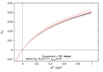
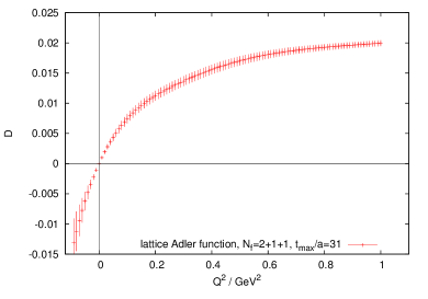
Figure 1: left panel: The renormalized vacuum polarization function from our lattice data ($a\approx 0.078\,\mathrm{fm},\,V=(2.5\,\mathrm{fm})^{3}$) together with a comparison to the dispersion relation data from [14]. right panel: The Adler function as derived from the lattice data; for illustration the upper summation limit was chosen maximal, i.e. $t_{\mathrm{max}}/a=T/2a-1=31$ and the spatial momentum is set to 0.

Here we compare our results, which are obtained at a single lattice spacing ($a\approx 0.078\,\mathrm{fm}$) with the results from [14] provided in the package alphaQED. At the stage of this first analysis, which is shown in the left panel of fig. 1 we find compelling agreement of results using the dispersion relation for $R(s)$ and lattice QCD results. With the known functional dependence on $\hat{K}^{2}$ of the $P_{n}$ of eq. (2) we can take the derivative w.r.t. $\hat{K}^{2}$ analytically and can also derive the Adler function from the lattice data. The result based on the same modified extrapolation of ref. [4] is shown in the right panel of Figure 1. Details of the limit $t_{\mathrm{max}}/a\to\infty$ as well as generalizations to different choices of non-zero momentum components will be discussed in a forthcoming publication.

3.2 Anomalous magnetic moment of the muon

Having obtained the HVP function, besides the Adler function a number of physical observables can be computed, see, e.g., Ref.[15]. Here we will focus on the leading-order HVP correction to the muon anomalous magnetic moment, $a_{\mu}^{\rm hvp}$, as an example to study the practical feasibility of the proposed analytic continuation method.

In lattice QCD $a_{\mu}^{\rm hvp}$ can be calculated through

$$a_{\mu}^{\rm hvp}=\alpha^{2}\int_{0}^{\infty}dK^{2}\;\frac{1}{K^{2}}f\left(\frac{K^{2}}{m_{\mu}^{2}}\right)(\Pi(K^{2})-\Pi(0))\;,$$ (3)

where $\alpha$ is the fine structure constant, $m_{\mu}$ is the muon mass, and $f(K^{2}/m_{\mu}^{2})$ is a known function [1]. To control the chiral extrapolation, we use a modified definition of $a_{\mu}^{\rm hvp}$ proposed in Refs. [4, 15],

$$a_{\bar{\mu}}^{\rm hvp}=\alpha^{2}\int_{0}^{\infty}dK^{2}\;\frac{1}{K^{2}}f\left(\frac{K^{2}}{m_{\mu}^{2}}\frac{H_{\rm phys}^{2}}{H^{2}}\right)(\Pi(K^{2})-\Pi(0))\;,$$ (4)

with $H=M_{V}$, i.e. the measured vector meson mass on the lattice. When the pion mass approaches its physical value, this vector meson mass becomes the physical $\rho$-meson mass, $M_{V}=M_{\rho}$. Then also $H=H_{\rm phys}$ and the modified definition, $a_{\bar{\mu}}^{\rm hvp}$ reproduces the value of $a_{\mu}^{\rm hvp}$ at the physical pion mass.

In the analytic continuation method, we can calculate the HVP function for a continuous momentum region $0<K^{2}<K_{\rm max}^{2}$, with $K_{\rm max}^{2}=\sum_{i=x,y,z}\hat{K}_{i}^{2}$ being the squared spatial momentum. In practice we split Eq. (4) into three parts:

$$a_{\bar{\mu}}^{\rm hvp} = a_{\bar{\mu}}^{(1)}+a_{\bar{\mu}}^{(2)}+a_{\bar{\mu}}^{(3)}\;,$$

$$a_{\bar{\mu}}^{(1)} = \alpha^{2}\int_{0}^{K_{\rm max}^{2}}dK^{2}\;\frac{1}{K^{2}}f\left(\frac{K^{2}}{m_{\mu}^{2}}\frac{H_{\rm phys}^{2}}{H^{2}}\right)(\Pi(K^{2})-\Pi(0))\;,$$

$$a_{\bar{\mu}}^{(2)} = \alpha^{2}\int_{K_{\rm max}^{2}}^{\infty}dK^{2}\;\frac{1}{K^{2}}f\left(\frac{K^{2}}{m_{\mu}^{2}}\frac{H_{\rm phys}^{2}}{H^{2}}\right)(\Pi(K_{\rm max}^{2})-\Pi(0))\;,$$

$$a_{\bar{\mu}}^{(3)} = \alpha^{2}\int_{K_{\rm max}^{2}}^{\infty}dK^{2}\;\frac{1}{K^{2}}f\left(\frac{K^{2}}{m_{\mu}^{2}}\frac{H_{\rm phys}^{2}}{H^{2}}\right)(\Pi(K^{2})-\Pi(K_{\rm max}^{2}))\;.$$ (5)

In Eq. (3.2), $a_{\bar{\mu}}^{(1)}+a_{\bar{\mu}}^{(2)}$ can be calculated directly using the analytic continuation method. Similar to the previous section, we can calculate $a_{\bar{\mu}}^{(1)}$ and $a_{\bar{\mu}}^{(2)}$ up to the value of $t_{\rm max}=\eta(T/2)$ with $\eta=3/4$ and estimate the finite-size effects using $\bar{\Pi}(K^{2};t>t_{\rm max})$.

The evaluation of $a_{\bar{\mu}}^{(3)}$ still requires a parametrization of $\bar{\Pi}(K^{2})$. This will bring in some model dependence in our analysis, which, however, is a small effect, since the total contribution of $a_{\bar{\mu}}^{(3)}$ only amounts to a few percent in case of momentum modes $|\vec{n}|^{2}=1,2,3$ where $\vec{n}$ classifies the momenta $\vec{k}=(2\pi/L)\vec{n}$ used in eq. (1). The exact parametrization of $\bar{\Pi}(K^{2})$ used in this calculation can be found in the Appendix of ref. [9].

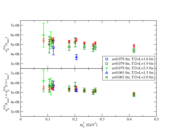
Figure 2: In this figure, the open symbols represent results from the analytic continuation method where we average over $|n|^{2}=1,2,3$. In the upper panel we use the range $-t_{\rm max}\leq t\leq t_{\rm max}$ only. The lower panel shows the results corrected for the estimated FSE. Our earlier data from the standard method of computing $a_{\mu}^{\rm hvp}$ are represented by filled symbols.

In Fig. 2 we show $a_{\bar{\mu}}^{\rm hvp}$ as a function of the squared pion mass. The results of $a_{\bar{\mu}}^{\rm hvp}$ calculated using Eq. (3.2) are shown by the empty symbols. These results have been averaged among various momentum modes ($|\vec{n}|^{2}=1,2,3$) and polarization directions. For comparison the results determined using our conventional approach of parameterizing the HVP function in the full momentum range are shown in the same figure, represented by the filled symbols. In the upper panel we show the results of $a_{\bar{\mu}}^{\rm hvp}(t_{\rm max})$, which are calculated using the correlator $C_{\mu\nu}(\vec{k},t)$ covering the range of $-t_{\rm max}\leq t\leq t_{\rm max}$. We look at the finite-size effects in $a_{\bar{\mu}}^{\rm hvp}(t_{\rm max})$ by comparing the results for different volumes. There are also some deviations between the results from the analytic continuation method and the standard parametrization method. To check for the finite-size effects, we evaluate the contribution to $a_{\bar{\mu}}^{\rm hvp}$ from $C_{\mu\nu}(\vec{k},t)$ at $|t|>t_{\rm max}$ leading to a correction $a_{\bar{\mu}}^{\rm hvp}(t>t_{\rm max})$. The corresponding results for $a_{\bar{\mu}}^{\rm hvp}(t_{\rm max})+a_{\bar{\mu}}^{\rm hvp}(t>t_{\rm max})$ are shown in the lower panel of Fig. 2. These results are consistent now among different lattice volumes. Besides this, the results from the analytic continuation method also agree with the ones from the standard parametrization method. As can be seen, the results from the analytic continuation method for $a_{\bar{\mu}}^{\rm hvp}$ show larger fluctuations than the standard ones. However, the analytic continuation method has the conceptual advantage that in the region of low $K^{2}$ the parametrization of $\bar{\Pi}(K^{2})$ can be avoided. Thus, we think that presently the analytic continuation method can serve as a valuable cross-check of the standard method to analyze the vacuum polarization function.

4 Conclusions and Outlook

In this proceedings contribution we discussed the analytic continuation method which, in principle, can provide information on the small momentum region for the vacuum polarization function or form factors in lattice QCD. In addition, it allows to access the space- and time-like momentum regions which in turn opens the possibility to compute scattering processes and resonances as an alternative to the finite size method of refs. [16, 17, 18]. Here we have given the examples of the Adler function and the anomalous magnetic moment of the muon $a_{\mu}^{\rm hvp}$ which we calculated by the analytic continuation method. When comparing to the standard method to compute $a_{\mu}^{\rm hvp}$ we found full agreement, but the analytic continuation method leads to noisier results. Still, we believe that the analytic continuation method is a valuable alternative which has, moreover, the potential to address other quantities where small or zero momenta are needed.

- [1] T. Blum. Lattice calculation of the lowest order hadronic contribution to the muon anomalous magnetic moment. Phys.Rev.Lett., 91:052001, 2003.
- [2] M. Gockeler et al. Vacuum polarisation and hadronic contribution to muon g-2 from lattice QCD. Nucl. Phys., B688:135–164, 2004.
- [3] C. Aubin and T. Blum. Calculating the hadronic vacuum polarization and leading hadronic contribution to the muon anomalous magnetic moment with improved staggered quarks. Phys. Rev., D75:114502, 2007.
- [4] Xu Feng, Karl Jansen, Marcus Petschlies, and Dru B. Renner. Two-flavor QCD correction to lepton magnetic moments at leading-order in the electromagnetic coupling. Phys.Rev.Lett., 107:081802, 2011.
- [5] Peter Boyle, Luigi Del Debbio, Eoin Kerrane, and James Zanotti. Lattice Determination of the Hadronic Contribution to the Muon using Dynamical Domain Wall Fermions. Phys.Rev., D85:074504, 2012.
- [6] Michele Della Morte, Benjamin Jager, Andreas Juttner, and Hartmut Wittig. Towards a precise lattice determination of the leading hadronic contribution to . JHEP, 1203:055, 2012.
- [7] Christopher Aubin, Thomas Blum, Maarten Golterman, and Santiago Peris. Model-independent parametrization of the hadronic vacuum polarization and g-2 for the muon on the lattice. Phys.Rev., D86:054509, 2012.
- [8] G.M. de Divitiis, R. Petronzio, and N. Tantalo. On the extraction of zero momentum form factors on the lattice. Phys.Lett., B718:589–596, 2012.
- [9] Xu Feng, Shoji Hashimoto, Grit Hotzel, Karl Jansen, Marcus Petschlies, et al. Computing the hadronic vacuum polarization function by analytic continuation. Phys.Rev., D88:034505, 2013.
- [10] X. D. Ji and C. W. Jung. Studying hadronic structure of the photon in lattice QCD. Phys. Rev. Lett., 86:208, 2001.
- [11] Harvey B. Meyer. Lattice QCD and the Timelike Pion Form Factor. Phys.Rev.Lett., 107:072002, 2011.
- [12] R. Baron et al. Light Meson Physics from Maximally Twisted Mass Lattice QCD. JHEP, 08:097, 2010.
- [13] R. Baron, Ph. Boucaud, J. Carbonell, A. Deuzeman, V. Drach, et al. Light hadrons from lattice QCD with light (u,d), strange and charm dynamical quarks. JHEP, 1006:111, 2010.
- [14] Fred Jegerlehner. Electroweak effective couplings for future precision experiments. Nuovo Cim., C034S1:31–40, 2011.
- [15] Dru B. Renner, Xu Feng, Karl Jansen, and Marcus Petschlies. Nonperturbative QCD corrections to electroweak observables. 2012.
- [16] M. Luscher. Volume Dependence of the Energy Spectrum in Massive Quantum Field Theories. 1. Stable Particle States. Commun.Math.Phys., 104:177, 1986.
- [17] M. Luscher. Volume Dependence of the Energy Spectrum in Massive Quantum Field Theories. 2. Scattering States. Commun.Math.Phys., 105:153–188, 1986.
- [18] Martin Luscher. Signatures of unstable particles in finite volume. Nucl.Phys., B364:237–254, 1991.