A Divide-and-Conquer Solver for Kernel Support Vector Machines

Abstract

The kernel support vector machine (SVM) is one of the most widely used classification methods; however, the amount of computation required becomes the bottleneck when facing millions of samples. In this paper, we propose and analyze a novel divide-and-conquer solver for kernel SVMs (DC-SVM). In the division step, we partition the kernel SVM problem into smaller subproblems by clustering the data, so that each subproblem can be solved independently and efficiently. We show theoretically that the support vectors identified by the subproblem solution are likely to be support vectors of the entire kernel SVM problem, provided that the problem is partitioned appropriately by kernel clustering. In the conquer step, the local solutions from the subproblems are used to initialize a global coordinate descent solver, which converges quickly as suggested by our analysis. By extending this idea, we develop a multilevel Divide-and-Conquer SVM algorithm with adaptive clustering and early prediction strategy, which outperforms state-of-the-art methods in terms of training speed, testing accuracy, and memory usage. As an example, on the covtype dataset with half-a-million samples, DC-SVM is 7 times faster than LIBSVM in obtaining the exact SVM solution (to within $10^{-6}$ relative error) which achieves 96.15% prediction accuracy. Moreover, with our proposed early prediction strategy, DC-SVM achieves about 96% accuracy in only 12 minutes, which is more than 100 times faster than LIBSVM.

1 Introduction

The support vector machine (SVM) (Cortes and Vapnik, 1995) is probably the most widely used classifier in varied machine learning applications. For problems that are not linearly separable, kernel SVM uses a “kernel trick” to implicitly map samples from input space to a high-dimensional feature space, where samples become linearly separable. Due to its importance, optimization methods for kernel SVM have been widely studied (Platt, 1998; Joachims, 1998), and efficient libraries such as LIBSVM (Chang and Lin, 2011) and SVMLight (Joachims, 1998) are well developed. However, the kernel SVM is still hard to scale up when the sample size reaches more than one million instances. The bottleneck stems from the high computational cost and memory requirements of computing and storing the kernel matrix, which in general is not sparse. By approximating the kernel SVM objective function, approximate solvers (Zhang et al., 2012; Le et al., 2013) avoid high computational cost and memory requirement, but suffer in terms of prediction accuracy.

In this paper, we propose a novel divide and conquer approach (DC-SVM) to efficiently solve the kernel SVM problem. DC-SVM achieves faster convergence speed compared to state-of-the-art exact SVM solvers, as well as better prediction accuracy in much less time than approximate solvers. To accomplish this performance, DC-SVM first divides the full problem into smaller subproblems, which can be solved independently and efficiently. We theoretically show that the kernel kmeans algorithm is able to minimize the difference between the solution of subproblems and of the whole problem, and support vectors identified by subproblems are very likely to be support vectors of the whole problem. However, running kernel kmeans on the whole dataset is time consuming, so we apply a two-step kernel kmeans procedure to efficiently find the partition. In the conquer step, the local solutions from the subproblems are “glued” together to yield an initial point for the global problem. As suggested by our analysis, the coordinate descent method in the final stage converges quickly to the global optimal.

Empirically, our proposed Divide-and-Conquer Kernel SVM solver can reduce the objective function value much faster than existing SVM solvers. For example, on the covtype dataset with half a million samples, DC-SVM can find an accurate globally optimal solution (to within $10^{-6}$ accuracy) within 3 hours on a single machine with 8 GBytes RAM, while the state-of-the-art solver LIBSVM takes more than 22 hours to achieve a similarly accurate solution (which yields 96.15% prediction accuracy). More interestingly, due to the closeness of the subproblem solutions to the global solution, we can employ an early prediction approach, using which DC-SVM can obtain high test accuracy extremely quickly. For example, on the covtype dataset, by using early prediction DC-SVM achieves 96.03% prediction accuracy within 12 minutes, while other solvers cannot achieve such performance in 10 hours.

The rest of the paper is outlined as follows. We propose the single-level DC-SVM in Section 3, and extend it to the multilevel version in Section 4. Experimental comparison with other state-of-the-art SVM solvers is shown in Section 5. The relationship between DC-SVM and other methods is discussed in Section 2, and the conclusions are given in Section 6. Extensive experimental comparisons are included in the Appendix.

2 Related Work

The optimization methods for SVM training has been intensively studied. Since training an SVM requires a large amount of memory, it is natural to apply decomposition methods (Platt, 1998), where only a subset of variables is updated at each step. Based on this idea, software packages such as LIBSVM (Chang and Lin, 2011) and SVMLight (Joachims, 1998) are well developed. To speed up the decomposition method, (Pérez-Cruz et al., 2004) proposed a double chunking approach to maintain a chunk of important samples, and the shrinking technique (Joachims, 1998) is also widely used to eliminate unimportant samples.

To speed up kernel SVM training on large-scale datasets, it is natural to divide the problem into smaller subproblems, and combine the models trained on each partition. (Jacobs et al., 1991) proposed a way to combine models, although in their algorithm subproblems are not trained independently, while (Tresp, 2000) discussed a Bayesian prediction scheme (BCM) for model combination. (Collobert et al., 2002) partition the training dataset arbitrarily in the beginning, and then iteratively refine the partition to obtain an approximate kernel SVM solution. (Kugler et al., 2006) applied the above ideas to solve multi-class problems. (Graf et al., 2005) proposed a multilevel approach (CascadeSVM): they randomly build a partition tree of samples and train the SVM in a “cascade” way: only support vectors in the lower level of the tree are passed to the upper level. However, no earlier method appears to discuss an elegant way to partition the data. In this paper, we theoretically show that kernel kmeans minimizes the error of the solution from the subproblems and the global solution. Based on this division step, we propose a simple method to combine locally trained SVM models, and show that the testing performance is better than BCM in terms of both accuracy and time (as presented in Table 1). More importantly, DC-SVM solves the original SVM problem, not just an approximated one. We compare our method with Cascade SVM in the experiments.

Another line of research proposes to reduce the training time by representing the whole dataset using a smaller set of landmark points, and clustering is an effective way to find landmark points (cluster centers). (Moody and Darken, 1989) proposed this idea to train the reduced sized problem with RBF kernel (LTPU); (Pavlov et al., 2000) used a similar idea as a preprocessing of the dataset, while (Yu et al., 2005) further generalized this approach to a hierarchical coarsen-refinement solver for SVM. Based on this idea, the kmeans Nyström method (Zhang et al., 2008) was proposed to approximate the kernel matrix using landmark points. (Boley and Cao, 2004) proposed to find samples with similar $\boldsymbol{\alpha}$ values by clustering, so both the clustering goal and training step are quite different from ours. All the above approaches focus on modeling the between-cluster (between-landmark points) relationships. In comparison, our method emphasizes on preserving the within-cluster relationships at the lower levels and explores the between-cluster information in the upper levels. We compare DC-SVM with LLSVM (using kmeans Nyström) and LTPU in Section 5.

There are many other approximate solvers for the kernel SVM, including kernel approximation approaches (Fine and Scheinberg, 2001; Zhang et al., 2012; Le et al., 2013), greedy basis selection (Keerthi et al., 2006), and online SVM solvers (Bordes et al., 2005). Recently, (Jose et al., 2013) proposed an approximate solver to reduce testing time, while our work is focused on reducing the training time of kernel SVM.

3 Divide and Conquer Kernel SVM with a single level

Given a set of instance-label pairs $({\boldsymbol{x}}_{i},y_{i}),i=1,\dots,n,{\boldsymbol{x}}_{i}\in{\mathbb{R}}^{d}$ and $y_{i}\in\{1,-1\}$, the main task in training the kernel SVM is to solve the following quadratic optimization problem:

$$\min_{\boldsymbol{\alpha}}f(\boldsymbol{\alpha})=\frac{1}{2}\boldsymbol{\alpha}^{T}Q\boldsymbol{\alpha}-{\boldsymbol{e}}^{T}\boldsymbol{\alpha},\ \text{ s.t. }0\leq\boldsymbol{\alpha}\leq C,$$ (1)

where ${\boldsymbol{e}}$ is the vector of all ones; $C$ is the balancing parameter between loss and regularization in the SVM primal problem; $\boldsymbol{\alpha}\in{\mathbb{R}}^{n}$ is the vector of dual variables; and $Q$ is an $n\times n$ matrix with $Q_{ij}=y_{i}y_{j}K({\boldsymbol{x}}_{i},{\boldsymbol{x}}_{j})$, where $K({\boldsymbol{x}}_{i},{\boldsymbol{x}}_{j})$ is the kernel function. Note that, as in (Keerthi et al., 2006; Joachims, 2006), we ignore the “bias” term – indeed, in our experiments reported in Section 5, we did not observe any improvement in test accuracy by including the bias term. Letting $\boldsymbol{\alpha}^{*}$ denote the optimal solution of (1), the decision value for a test data ${\boldsymbol{x}}$ can be computed by $\sum_{i=1}^{n}\alpha_{i}^{*}y_{i}K({\boldsymbol{x}},{\boldsymbol{x}}_{i})$.

We begin by describing the single-level version of our proposed algorithm. The main idea behind our divide and conquer SVM solver (DC-SVM) is to divide the data into smaller subsets, where each subset can be handled efficiently and independently. The subproblem solutions are then used to initialize a coordinate descent solver for the whole problem. To do this, we first partition the dual variables into $k$ subsets $\{{\mathcal{V}}_{1},\dots,{\mathcal{V}}_{k}\}$, and then solve the respective subproblems independently

$$\min_{\boldsymbol{\alpha}_{(c)}}\!\frac{1}{2}(\boldsymbol{\alpha}_{(c)})^{T}Q_{(c,c)}\boldsymbol{\alpha}_{(c)}\!-\!{\boldsymbol{e}}^{T}\boldsymbol{\alpha}_{(c)},\text{ s.t. }0\!\leq\!\boldsymbol{\alpha}_{(c)}\!\leq\!C,$$ (2)

where $c=1,\dots,k$, $\boldsymbol{\alpha}_{(c)}$ denotes the subvector $\{\alpha_{p}\mid p\in{\mathcal{V}}_{c}\}$ and $Q_{(c,c)}$ is the submatrix of $Q$ with row and column indexes ${\mathcal{V}}_{c}$.

The quadratic programming problem (1) has $n$ variables, and generally takes $O(n^{3})$ time to solve. By dividing it into $k$ subproblems (2) with equal sizes, the time complexity for solving the subproblems can be dramatically reduced to $O(k\cdot(\frac{n}{k})^{3})=O(n^{3}/k^{2})$. Moreover, the space requirement is also reduced from $O(n^{2})$ to $O(n^{2}/k^{2})$.

After computing all the subproblem solutions, we concatenate them to form an approximate solution for the whole problem $\bar{\boldsymbol{\alpha}}=[\bar{\boldsymbol{\alpha}}_{(1)},\dots,\bar{\boldsymbol{\alpha}}_{(k)}]$, where $\bar{\boldsymbol{\alpha}}_{(c)}$ is the optimal solution for the $c$-th subproblem. In the conquer step, $\bar{\boldsymbol{\alpha}}$ is used to initialize the solver for the whole problem. We show that this procedure achieves faster convergence due to the following reasons: (1) $\bar{\boldsymbol{\alpha}}$ is close to the optimal solution for the whole problem ${\boldsymbol{\alpha}}^{*}$, so the solver only requires a few iterations to converge (see Theorem 1); (2) the set of support vectors of the subproblems is expected to be close to the set of support vectors of the whole problem (see Theorem 2). Hence, the coordinate descent solver for the whole problem converges very quickly.

Divide Step. We now discuss in detail how to divide problem (1) into subproblems. In order for our proposed method to be efficient, we require $\bar{\boldsymbol{\alpha}}$ to be close to the optimal solution of the original problem $\boldsymbol{\alpha}^{*}$. In the following, we derive a bound on $\|\bar{\boldsymbol{\alpha}}-\boldsymbol{\alpha}^{*}\|_{2}$ by first showing that $\bar{\boldsymbol{\alpha}}$ is the optimal solution of (1) with an approximate kernel.

Lemma 1.

$\bar{\boldsymbol{\alpha}}$ is the optimal solution of (1) with kernel function $K({\boldsymbol{x}}_{i},{\boldsymbol{x}}_{j})$ replaced by

$$\bar{K}({\boldsymbol{x}}_{i},{\boldsymbol{x}}_{j})=I(\pi({\boldsymbol{x}}_{i}),\pi({\boldsymbol{x}}_{j}))K({\boldsymbol{x}}_{i},{\boldsymbol{x}}_{j}),$$ (3)

where $\pi({\boldsymbol{x}}_{i})$ is the cluster that ${\boldsymbol{x}}_{i}$ belongs to; $I(a,b)=1$ iff $a=b$ and $I(a,b)=0$ otherwise.

Proof.

When using $\bar{K}$ defined in (3), the matrix $Q$ in (1) becomes $\bar{Q}$ as given below:

$$\bar{Q}_{i,j}=\begin{cases}y_{i}y_{j}K({\boldsymbol{x}}_{i},{\boldsymbol{x}}_{j}),&\text{ if }\pi({\boldsymbol{x}}_{i})=\pi({\boldsymbol{x}}_{j}),\\ 0,&\text{ if }\pi({\boldsymbol{x}}_{i})\neq\pi({\boldsymbol{x}}_{j}).\end{cases}$$ (4)

Therefore, the quadratic term in (1) can be decomposed into

$$\boldsymbol{\alpha}^{T}\bar{Q}\boldsymbol{\alpha}=\sum_{c=1}^{k}\boldsymbol{\alpha}_{(c)}^{T}Q_{(c,c)}\boldsymbol{\alpha}_{(c)}.$$

The constraints and linear term in (1) are also decomposable, so the subproblems are independent, and concatenation of their optimal solutions, $\bar{\boldsymbol{\alpha}}$, is the optimal solution for (1) when $K$ is replaced by $\bar{K}$. ∎

Based on the above lemma, we are able to bound $\|\boldsymbol{\alpha}^{*}-\bar{\boldsymbol{\alpha}}\|_{2}$ by the sum of between-cluster kernel values:

Theorem 1.

Given data points ${\boldsymbol{x}}_{1},\dots,{\boldsymbol{x}}_{n}$ and a partition indicator $\{\pi({\boldsymbol{x}}_{1}),\dots,\pi({\boldsymbol{x}}_{n})\}$,

$$0\leq f(\bar{\boldsymbol{\alpha}})-f(\boldsymbol{\alpha}^{*})\leq(1/2)C^{2}D(\pi),$$ (5)

where $f(\boldsymbol{\alpha})$ is the objective function in (1), $\bar{\boldsymbol{\alpha}}$ is as in Lemma 1, $\boldsymbol{\alpha}^{*}$ is the global optimal of (1) and $D(\pi)=\sum_{i,j:\pi({\boldsymbol{x}}_{i})\neq\pi({\boldsymbol{x}}_{j})}|K({\boldsymbol{x}}_{i},{\boldsymbol{x}}_{j})|$. Furthermore, $\|\boldsymbol{\alpha}^{*}-\bar{\boldsymbol{\alpha}}\|_{2}^{2}\leq C^{2}D(\pi)/\sigma_{n}$ where $\sigma_{n}$ is the smallest eigenvalue of the kernel matrix.

Proof.

We use $\bar{f}(\boldsymbol{\alpha})$ to denote the objective function of (1) with kernel $\bar{K}$. By Lemma 1, $\bar{\boldsymbol{\alpha}}$ is the minimizer of (1) with $K$ replaced by $\bar{K}$, thus $\bar{f}(\bar{\boldsymbol{\alpha}})\leq\bar{f}(\boldsymbol{\alpha}^{*})$. By the definition of $\bar{f}(\boldsymbol{\alpha}^{*})$ we can easily show that

$$\bar{f}(\boldsymbol{\alpha}^{*})=f(\boldsymbol{\alpha}^{*})-\frac{1}{2}\sum_{i,j:\pi({\boldsymbol{x}}_{i})\neq\pi({\boldsymbol{x}}_{j})}\alpha^{*}_{i}\alpha^{*}_{j}y_{i}y_{j}K({\boldsymbol{x}}_{i},{\boldsymbol{x}}_{j})$$ (6)

Similarly, we have

$$\bar{f}(\bar{\boldsymbol{\alpha}})=f(\bar{\boldsymbol{\alpha}})-\frac{1}{2}\sum_{i,j:\pi({\boldsymbol{x}}_{i})\neq\pi({\boldsymbol{x}}_{j})}\bar{\alpha}_{i}\bar{\alpha}_{j}y_{i}y_{j}K({\boldsymbol{x}}_{i},{\boldsymbol{x}}_{j}),$$ (7)

Combining with $\bar{f}(\bar{\boldsymbol{\alpha}})\leq\bar{f}(\boldsymbol{\alpha}^{*})$ we have

$$f(\bar{\boldsymbol{\alpha}}) \leq\bar{f}(\boldsymbol{\alpha}^{*})+\frac{1}{2}\sum_{i,j:\pi({\boldsymbol{x}}_{i})\neq\pi({\boldsymbol{x}}_{j})}\bar{\alpha}_{i}\bar{\alpha}_{j}y_{i}y_{j}K({\boldsymbol{x}}_{i},{\boldsymbol{x}}_{j}),$$

$$=f(\boldsymbol{\alpha}^{*})+\frac{1}{2}\!\!\sum_{i,j:\pi({\boldsymbol{x}}_{i})\neq\pi({\boldsymbol{x}}_{j})}\!\!\!\!\!\!(\bar{\alpha}_{i}\bar{\alpha_{j}}-\alpha^{*}_{i}\alpha^{*}_{j})y_{i}y_{j}K({\boldsymbol{x}}_{i},{\boldsymbol{x}}_{j})$$ (8)

$$\leq f(\boldsymbol{\alpha}^{*})\!+\!\frac{1}{2}C^{2}D(\pi),\text{ since }0\leq\bar{\alpha}_{i},\alpha^{*}_{i}\leq C\ \text{for all }i.$$

Also, since $\boldsymbol{\alpha}^{*}$ is the optimal solution of (1) and $\bar{\boldsymbol{\alpha}}$ is a feasible solution, $f(\boldsymbol{\alpha}^{*})\leq f(\bar{\boldsymbol{\alpha}})$, thus proving the first part of the theorem.

Let $\sigma_{n}$ be the smallest singular value of the positive definite kernel matrix $K$. Since $Q=\text{diag}({\boldsymbol{y}})K\text{diag}({\boldsymbol{y}})$, $Q$ and $K$ have identical singular values. Suppose we write $\bar{\boldsymbol{\alpha}}=\boldsymbol{\alpha}^{*}+\Delta\boldsymbol{\alpha}$,

$$f(\bar{\boldsymbol{\alpha}})=f(\boldsymbol{\alpha}^{*})+(\boldsymbol{\alpha}^{*})^{T}Q\Delta\boldsymbol{\alpha}+\frac{1}{2}(\Delta\boldsymbol{\alpha})^{T}Q\Delta\boldsymbol{\alpha}-{\boldsymbol{e}}^{T}\Delta\boldsymbol{\alpha}.$$

The optimality condition for (1) is

$$\nabla_{i}f(\boldsymbol{\alpha}^{*})\begin{cases}=0&\text{ if }0<\alpha^{*}_{i}<C,\\ \geq 0&\text{ if }\alpha^{*}_{i}=0,\\ \leq 0&\text{ if }\alpha^{*}_{i}=C,\end{cases}$$ (9)

where $\nabla f(\boldsymbol{\alpha}^{*})=Q\boldsymbol{\alpha}^{*}-{\boldsymbol{e}}$. Since $\bar{\boldsymbol{\alpha}}$ is a feasible solution, it is easy to see that $(\Delta\boldsymbol{\alpha})_{i}\geq 0$ if $\alpha^{*}_{i}=0$, and $(\Delta\boldsymbol{\alpha})_{i}\leq 0$ if $\alpha^{*}_{i}=C$. Thus,

$$(\Delta\boldsymbol{\alpha})^{T}(Q\boldsymbol{\alpha}^{*}-{\boldsymbol{e}})=\sum_{i=1}^{n}(\Delta\boldsymbol{\alpha})_{i}((Q\boldsymbol{\alpha}^{*})_{i}-1)\geq 0.\\$$

So $f(\bar{\boldsymbol{\alpha}})\geq f(\boldsymbol{\alpha}^{*})+\frac{1}{2}\Delta\boldsymbol{\alpha}^{T}Q\Delta\boldsymbol{\alpha}\geq f(\boldsymbol{\alpha}^{*})+\frac{1}{2}\sigma_{n}\|\Delta\boldsymbol{\alpha}\|_{2}^{2}$. Since we already know that $f(\bar{\boldsymbol{\alpha}})\leq f(\boldsymbol{\alpha}^{*})+\frac{1}{2}C^{2}D(\{{\boldsymbol{x}}_{i}\}_{i=1}^{n},\pi)$, this implies $\|\boldsymbol{\alpha}^{*}-\bar{\boldsymbol{\alpha}}\|_{2}^{2}\leq C^{2}D(\pi)/\sigma_{n}$. ∎

In order to minimize $\|\boldsymbol{\alpha}^{*}-\bar{\boldsymbol{\alpha}}\|$, we want to find a partition with small $D(\pi)$. Moreover, a balanced partition is preferred to achieve faster training speed. This can be done by the kernel kmeans algorithm, which aims to minimize the off-diagonal values of the kernel matrix with a balancing normalization.

We now show that the bound derived in Theorem 1 is reasonably tight in practice. On a subset (10000 instances) of the covtype data, we try different numbers of clusters $k=8,16,32,64,128$; for each $k$, we use kernel kmeans to obtain the data partition $\{{\mathcal{V}}_{1},\dots,{\mathcal{V}}_{k}\}$, and then compute $C^{2}D(\pi)/2$ (the right hand side of (5)) and $f(\bar{\boldsymbol{\alpha}})-f(\boldsymbol{\alpha}^{*})$ (the left hand side of (5)). The results are presented in Figure 1. The left panel shows the bound (in red) and the difference in objectives $f(\bar{\boldsymbol{\alpha}})-f(\boldsymbol{\alpha}^{*})$ in absolute scale, while the right panel shows these values in a log scale. Figure 1 shows that the bound is quite close to the difference in objectives in an absolute sense (the red and blue curves nearly overlap), especially compared to the difference in objectives when the data is partitioned randomly (this also shows effectiveness of the kernel kmeans procedure). Thus, our data partitioning scheme and subsequent solution of the subproblems leads to good approximations to the global kernel SVM problem.

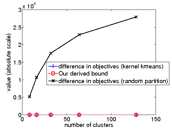
(a) covtype 10000 samples.

(b) covtype 10000 samples (log scale).

Figure 1: Demonstration of the bound in Theorem 1 – our data partitioning scheme leads to good approximations to the global solution $\boldsymbol{\alpha}^{*}$. The left plot is on an absolute scale, while the right one is on a logarithmic scale.

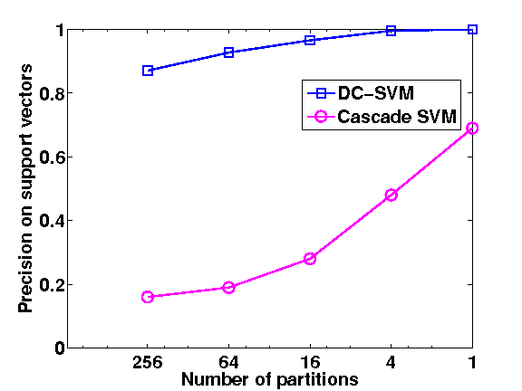
(a) rbf kernel, precision

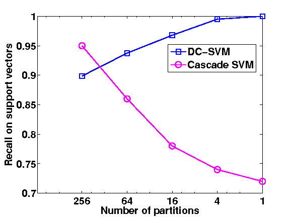
(b) rbf kernel, recall

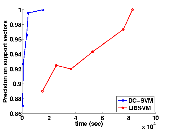
(c) rbf kernel, time vs. precision

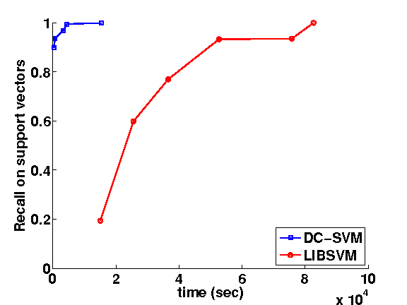
(d) rbf kernel, time vs. recall

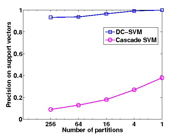
(e) polynomial kernel, precision

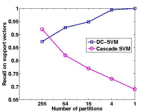
(f) polynomial kernel, recall

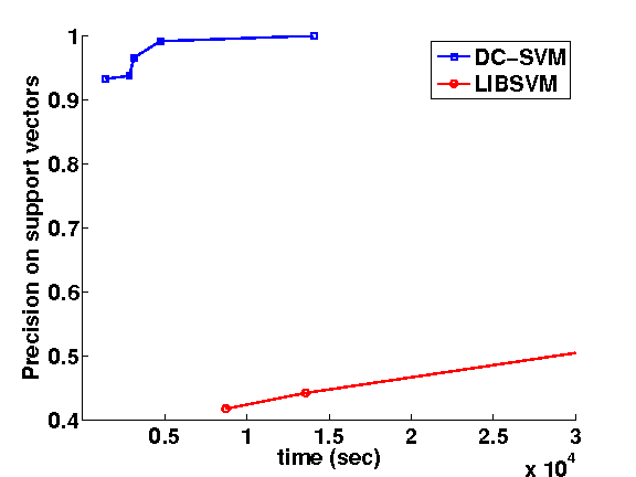
(g) polynomial kernel, time vs. precision

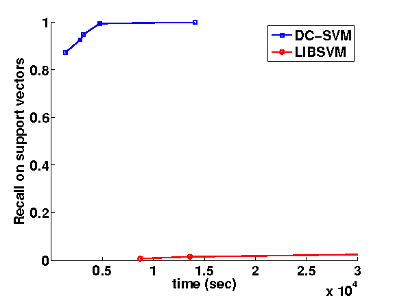
(h) polynomial kernel, time vs. recall

Figure 2: Our multilevel DC-SVM algorithm computes support vectors for subproblems during the “conquer” phase. The above plots show that DC-SVM identifies support vectors more accurately (Figure 2a, 2b, 2e, 2f) than cascade SVM, and more quickly than the shrinking strategy in LIBSVM.

However, kernel kmeans has $O(n^{2}d)$ time complexity, which is too expensive for large-scale problems. Therefore we consider a simple two-step kernel kmeans approach as in (Ghitta et al., 2011). The two-step kernel kmeans algorithm first runs kernel kmeans on $m$ randomly sampled data points ($m\ll n$) to construct cluster centers in the kernel space. Based on these centers, each data point computes its distance to cluster centers and decides which cluster it belongs to. The algorithm has time complexity $O(nmd)$ and space complexity $O(m^{2})$.

A key facet of our proposed divide and conquer algorithm is that the set of support vectors from the subproblems $\bar{S}:=\{i\mid\bar{\alpha}_{i}>0\}$, where $\bar{\alpha}_{i}$ is the $i$-th element of $\bar{\boldsymbol{\alpha}}$, is very close to that of the whole problem $S:=\{i\mid\alpha^{*}_{i}>0\}$. Letting $\bar{f}(\boldsymbol{\alpha})$ denote the objective function of (1) with kernel $\bar{K}$ defined in (3), the following theorem shows that when $\bar{\alpha}_{i}=0$ (${\boldsymbol{x}}_{i}$ is not a support vector of the subproblem) and $\nabla_{i}\bar{f}(\bar{\boldsymbol{\alpha}})$ is large enough, then ${\boldsymbol{x}}_{i}$ will not be a support vector of the whole problem.

Theorem 2.

For any $i\in\{1,\dots,n\}$, if $\bar{\alpha}_{i}=0$ and

$$\nabla_{i}\bar{f}(\bar{\boldsymbol{\alpha}})>CD(\pi)(1+\sqrt{n}K_{max}/\sqrt{\sigma_{n}D(\pi)}),$$

where $K_{max}=\max_{i}K({\boldsymbol{x}}_{i},{\boldsymbol{x}}_{i})$, then ${\boldsymbol{x}}_{i}$ will not be a support vector of the whole problem, i.e., $\alpha^{*}_{i}=0$.

Proof.

Let $\Delta Q=Q-\bar{Q}$ and $\Delta\boldsymbol{\alpha}=\boldsymbol{\alpha}^{*}-\bar{\boldsymbol{\alpha}}$. From the optimality condition for (1) (see (9)), we know that $\alpha^{*}_{i}=0$ if $(Q\boldsymbol{\alpha}^{*})_{i}>1$. Since $Q\boldsymbol{\alpha}^{*}=(\bar{Q}+\Delta Q)(\bar{\boldsymbol{\alpha}}+\Delta\boldsymbol{\alpha})$, we see that

$$(Q\boldsymbol{\alpha}^{*})_{i} =(\bar{Q}\bar{\boldsymbol{\alpha}})_{i}+(\Delta Q\bar{\boldsymbol{\alpha}})_{i}+((\bar{Q}+\Delta Q)\Delta\boldsymbol{\alpha})_{i}.$$

$$=(\bar{Q}\bar{\boldsymbol{\alpha}})_{i}+\sum_{j:\pi({\boldsymbol{x}}_{i})\neq\pi({\boldsymbol{x}}_{j})}y_{i}y_{j}K({\boldsymbol{x}}_{i},{\boldsymbol{x}}_{j})\bar{\alpha}_{j}+\sum_{j}y_{i}y_{j}K({\boldsymbol{x}}_{i},{\boldsymbol{x}}_{j})(\Delta\boldsymbol{\alpha})_{j}$$

$$\geq(\bar{Q}\bar{\boldsymbol{\alpha}})_{i}-CD(\pi)-K_{max}\|\Delta\boldsymbol{\alpha}\|_{1}$$

$$\geq(\bar{Q}\bar{\boldsymbol{\alpha}})_{i}-CD(\pi)-\sqrt{n}K_{max}C\sqrt{D(\pi)}/\sqrt{\sigma_{n}}$$

$$=(\bar{Q}\bar{\boldsymbol{\alpha}})_{i}-CD(\pi)\left(1+\frac{\sqrt{n}K_{max}}{\sqrt{\sigma_{n}D(\pi)}}\right).$$

The condition stated in the theorem implies $(\bar{Q}\bar{\boldsymbol{\alpha}})_{i}>1+CD(\pi)(1+\frac{\sqrt{n}K_{max}}{\sqrt{\sigma_{n}D(\pi)}})$, which implies $(Q\boldsymbol{\alpha}^{*})_{i}-1>0$, so from the optimality condition (9), $\alpha^{*}_{i}=0$. ∎

In practice also, we observe that DC-SVM can identify the set of support vectors of the whole problem very quickly. Figure 2 demonstrates that DC-SVM identifies support vectors much faster than the shrinking strategy implemented in LIBSVM (Chang and Lin, 2011) (we discuss these results in more detail in Section 4).

Conquer Step. After computing $\bar{\boldsymbol{\alpha}}$ from the subproblems, we use $\bar{\boldsymbol{\alpha}}$ to initialize the solver for the whole problem. In principle, we can use any SVM solver in our divide and conquer framework, but we focus on using coordinate descent method as in LIBSVM to solve the whole problem. The main idea is to update one variable at a time, and always choose the $\alpha_{i}$ with the largest gradient value to update. The benefit of applying coordinate descent is that we can avoid a lot of unnecessary access to the kernel matrix entries if $\alpha_{i}$ never changes from zero to nonzero. Since $\bar{\boldsymbol{\alpha}}$’s are close to $\boldsymbol{\alpha}^{*}$, the $\bar{\boldsymbol{\alpha}}$-values for most vectors that are not support vectors will not become nonzero, and so the algorithm converges quickly.

4 Divide and Conquer SVM with multiple levels

There is a trade-off in choosing the number of clusters $k$ for a single-level DC-SVM with only one divide and conquer step. When $k$ is small, the subproblems have similar sizes as the original problem, so we will not gain much speedup. On the other hand, when we increase $k$, time complexity for solving subproblems can be reduced, but the resulting $\bar{\boldsymbol{\alpha}}$ can be quite different from $\boldsymbol{\alpha}^{*}$ according to Theorem 1, so the conquer step will be slow. Therefore, we propose to run DC-SVM with multiple levels to further reduce the time for solving the subproblems, and meanwhile still obtain $\bar{\boldsymbol{\alpha}}$ values that are close to $\boldsymbol{\alpha}^{*}$.

In multilevel DC-SVM, at the $l$-th level, we partition the whole dataset into $k^{l}$ clusters $\{{\mathcal{V}}^{(l)}_{1},\dots,{\mathcal{V}}^{(l)}_{k^{l}}\}$, and solve those $k^{l}$ subproblems independently to get $\bar{\boldsymbol{\alpha}}^{(l)}$. In order to solve each subproblem efficiently, we use the solutions from the lower level $\bar{\boldsymbol{\alpha}}^{(l+1)}$ to initialize the solver at the $l$-th level, so each level requires very few iterations. This allows us to use small values of $k$, for example, we use $k=4$ for all the experiments. In the following, we discuss more insights to further speed up our procedure.

Adaptive Clustering. The two-step kernel kmeans approach has time complexity $O(nmd)$, so the number of samples $m$ cannot be too large. In our implementation we use $m=1000$. When the data set is very large, the performance of two-step kernel kmeans may not be good because we sample only a few data points. This will influence the performance of DC-SVM.

To improve the clustering for DC-SVM, we propose the following adaptive clustering approach. The main idea is to explore the sparsity of $\boldsymbol{\alpha}$ in the SVM problem, and sample from the set of support vectors to perform two-step kernel kmeans. The number of support vectors is generally much smaller than $n$ because of the bound constraints. Suppose we are at the $l$-th level, and the current set of support vectors is defined by $\bar{S}=\{i\mid\bar{\alpha}_{i}>0\}$. Suppose the set of support vectors for the final solution is given by $S^{*}=\{i\mid\alpha^{*}_{i}>0\}$. We can define the sum of off-diagonal elements on $\bar{S}\cup S^{*}$ as $D_{S^{*}\cup\bar{S}}(\pi)=\sum_{i,j\in S^{*}\cup\bar{S}\text{ and }\pi({\boldsymbol{x}}_{i})\neq\pi({\boldsymbol{x}}_{j})}|K({\boldsymbol{x}}_{i},{\boldsymbol{x}}_{j})|$. The following theorem shows that we can refine the bound in Theorem 1:

Theorem 3.

Given data points ${\boldsymbol{x}}_{1},\dots,{\boldsymbol{x}}_{n}$ and a partition $\{{\mathcal{V}}_{1},\dots,{\mathcal{V}}_{k}\}$ with indicators $\pi$,

$$0\leq f(\bar{\boldsymbol{\alpha}})-f(\boldsymbol{\alpha}^{*})\leq(1/2)C^{2}D_{S^{*}\cup\bar{S}}(\pi).$$

Furthermore, $\|\boldsymbol{\alpha}^{*}-\bar{\boldsymbol{\alpha}}\|_{2}^{2}\leq C^{2}D_{S^{*}\cup\bar{S}}(\pi)/\sigma_{n}$.

Proof.

Similar to the proof in Theorem 1, we use $\bar{f}(\boldsymbol{\alpha})$ to denote the objective function of (1) with kernel $\bar{K}$. Combine (8) with the fact that $\alpha^{*}_{i}=0\ \ \forall i\notin S^{*}$ and $\bar{\alpha}_{i}=0\ \ \forall i\notin\bar{S}$, we have

$$f(\bar{\boldsymbol{\alpha}}) \leq f(\boldsymbol{\alpha}^{*})-\frac{1}{2}\sum_{i,j:\pi({\boldsymbol{x}}_{i})\neq\pi({\boldsymbol{x}}_{j})\text{ and }i,j\in S^{*}}(\bar{\alpha}_{i}\bar{\alpha}_{j}-\alpha^{*}_{i}\alpha^{*}_{j})y_{i}y_{j}K({\boldsymbol{x}}_{i},{\boldsymbol{x}}_{j})$$

$$\leq f(\boldsymbol{\alpha}^{*})+\frac{1}{2}C^{2}D_{S^{*}\cup\bar{S}}(\pi).$$

The second part of the proof is identical to the proof of the second part of Theorem 1. ∎

The above observations suggest that if we know the set of support vectors $\bar{S}$ and $S^{*}$, $\|\boldsymbol{\alpha}^{*}-\bar{\boldsymbol{\alpha}}\|$ only depends on whether we can obtain a good partition of $\bar{S}\cup S^{*}$. Therefore, we can sample $m$ points from $\bar{S}\cup S^{*}$ instead of the whole dataset to perform the clustering. The performance of two-step kernel kmeans depends on the sampling rate; we reduce the sampling rate from $m/n$ to $m/|S^{*}\cup\bar{S}|$. As a result, the performance significantly improves when $|S^{*}\cup\bar{S}|\ll n$.

In practice we do not know $S^{*}$ or $\bar{S}$ before solving the problem. However, both Theorem 2 and experiments shown in Figure 2 suggest that we have a good guess of support vectors even at the bottom level. Therefore, we can use the lower level support vectors as a good guess of the upper level support vectors. More specifically, after computing $\bar{\boldsymbol{\alpha}}^{l}$ from level $l$, we can use its support vector set $\bar{S}^{l}:=\{i\mid\bar{\alpha}_{i}^{l}>0\}$ to run two-step kernel kmeans for finding the clusters at the $(l-1)$-th level. Using this strategy, we obtain progressively better partitioning as we approach the original problem at the top level.

Table 1: Comparing prediction methods using a lower level model. Our proposed early prediction strategy is better in terms of prediction accuracy and testing time per sample (time given in milliseconds).

	webspam $k=50$	webspam $k=100$	covtype $k=50$	covtype $k=100$
Prediction by (10)	92.6% / 1.3ms	89.5% / 1.3ms	94.6% / 2.6ms	92.7% / 2.6ms
BCM in (Tresp, 2000)	98.4% / 2.5ms	95.3% / 3.3ms	91.5% / 3.7ms	89.3% / 5.6ms
Early Prediction by (11)	99.1% / .17ms	99.0% / .16ms	96.1% / .4ms	96.0% / .2ms

Early identification of support vectors. We first run LIBSVM to obtain the final set of support vectors, and then run DC-SVM with various numbers of clusters $4^{5},4^{4},\dots,4^{0}$ (corresponding to level $5,4,\dots,1$ for multilevel DC-SVM). We show the precision and recall for the $\bar{\boldsymbol{\alpha}}$ at each level in identifying support vectors. Figure 2 shows that DC-SVM can identify about 90% support vectors even using $256$ clusters. As discussed in Section 2, Cascade SVM (Graf et al., 2005) is another way to identify support vectors. However, it is clear from Figure 2 that Cascade SVM cannot identify support vectors accurately as (1) it does not use kernel kmeans clustering, and (2) it cannot correct the false negative error made in lower levels. Figure 2c, 2d, 2g, 2h further shows that DC-SVM identifies support vectors more quickly than the shrinking strategy in LIBSVM.

Early prediction based on the $l$-th level solution. Computing the exact kernel SVM solution can be quite time consuming, so it is important to obtain a good model using limited time and memory. We now propose a way to efficiently predict the label of unknown instances using the lower-level models $\bar{\boldsymbol{\alpha}}^{l}$. We will see in the experiments that prediction using $\bar{\boldsymbol{\alpha}}^{l}$ from a lower level $l$ already can achieve near-optimal testing performance.

When the $l$-th level solution $\bar{\boldsymbol{\alpha}}^{l}$ is computed, a single naive way to predict a new instance ${\boldsymbol{x}}$’s label $\tilde{y}$ is:

$$\tilde{y}=\text{sign}\left(\sum_{i=1}^{n}y_{i}\bar{\alpha}^{l}_{i}K({\boldsymbol{x}},{\boldsymbol{x}}_{i})\right).$$ (10)

Another way to combine the models trained from $k$ clusters is to use the probabilistic framework proposed in the Bayesian Committee Machine (BCM) (Tresp, 2000). However, as we show below, both these methods do not give good prediction accuracy when the number of clusters is large.

Instead, we propose the following early prediction strategy. From Lemma 1, $\bar{\boldsymbol{\alpha}}$ is the optimal solution to the SVM dual problem (1) on the whole dataset with the approximated kernel $\bar{K}$ defined in (3). Therefore, we propose to use the same kernel function $\bar{K}$ in the testing phase, which leads to the prediction

$$\sum_{c=1}^{k}\sum_{i\in{\mathcal{V}}_{c}}y_{i}\alpha_{i}\bar{K}({\boldsymbol{x}}_{i},{\boldsymbol{x}})=\sum_{i\in{\mathcal{V}}_{\pi({\boldsymbol{x}})}}y_{i}\alpha_{i}K({\boldsymbol{x}}_{i},{\boldsymbol{x}}),$$ (11)

where $\pi({\boldsymbol{x}})$ can be computed by finding the nearest cluster center. Therefore, the testing procedure for early prediction is: (1) find the nearest cluster that $x$ belongs to, and then (2) use the model trained by data within that cluster to compute the decision value.

We compare this method with prediction by (10) and BCM in Table 1. The results show that our proposed testing scheme is better in terms of test accuracy. We also compare average testing time per instance in Table 1, and our proposed method is much more efficient as we only evaluate $K({\boldsymbol{x}},{\boldsymbol{x}}_{i})$ for all ${\boldsymbol{x}}_{i}$ in the same cluster as ${\boldsymbol{x}}$, thus reducing the testing time from $O(|S|d)$ to $O(|S|d/k)$, where $S$ is the set of support vectors.

Refine solution before solving the whole problem. Before training the final model at the top level using the whole dataset, we can refine the initialization by solving the SVM problem induced by all support vectors at the first level, i.e., level below the final level. As proved in Theorem 2, the support vectors of lower level models are likely to be the support vectors of the whole model, so this will give a more accurate solution, and only requires us to solve a problem with $O(|\bar{S}^{(1)}|)$ samples, where $\bar{S}^{(1)}$ is the support vectors at the first level. Our final algorithm is given in Algorithm 1.

Input : Training data $\{({\boldsymbol{x}}_{i},y_{i})\}_{i=1}^{n}$, balancing parameter $C$, kernel function.

Output : The SVM dual solution $\boldsymbol{\alpha}$.

for $l=l^{\text{max}},\dots,1$ do

      Set number of clusters in the current level $k_{l}=k^{l}$;

      if $l=l^{\text{max}}$ then

           Sample $m$ points $\{{\boldsymbol{x}}_{i_{1}},\dots,{\boldsymbol{x}}_{i_{m}}\}$ from the whole training set;

          

           else

                Sample $m$ points $\{{\boldsymbol{x}}_{i_{1}},\dots,{\boldsymbol{x}}_{i_{m}}\}$ from $\{{\boldsymbol{x}}_{i}\mid\bar{\alpha}^{(l+1)}_{i}>0\}$;

               

                end if

               

               Run kernel kmeans on $\{{\boldsymbol{x}}_{i_{1}},\dots,{\boldsymbol{x}}_{i_{m}}\}$ to get cluster centers ${\boldsymbol{c}}_{1},\dots,{\boldsymbol{c}}_{k^{l}}$;

                Obtain partition ${\mathcal{V}}_{1},\dots,{\mathcal{V}}_{k^{l}}$ for all data points ;

                for $c=1,\dots,k^{l}$ do

                     Obtain $\bar{\boldsymbol{\alpha}}^{(l)}_{{\mathcal{V}}_{c}}$ by solving SVM for the data in the $c$-th cluster ${\mathcal{V}}_{c}$ with $\bar{\boldsymbol{\alpha}}^{(l+1)}_{{\mathcal{V}}_{c}}$ as the initial point ( $\bar{\boldsymbol{\alpha}}^{l_{\text{max}}+1}_{{\mathcal{V}}_{c}}$ is set to 0);

                    

                     end for

                    

                     end for

                    Refine solution: Compute $\boldsymbol{\alpha}^{(0)}$ by solving SVM on $\{{\boldsymbol{x}}_{i}\mid\alpha^{(1)}_{i}\neq 0\}$ using $\boldsymbol{\alpha}^{(1)}$ as the initial point;

                     Solve SVM on the whole data using $\boldsymbol{\alpha}^{(0)}$ as the initial point;

Algorithm 1 Divide and Conquer SVM

5 Experimental Results

Table 2: Dataset statistics

dataset	Number of	Number of	d
	training samples	testing samples
ijcnn1	49,990	91,701	22
cifar	50,000	10,000	3072
census	159,619	39,904	409
covtype	464,810	116,202	54
webspam	280,000	70,000	254
kddcup99	4,898,431	311,029	125
mnist8m	8,000,000	100,000	784

We now compare our proposed algorithm with other SVM solvers. All the experiments are conducted on an Intel Xeon X5355 2.66GHz CPU with 8G RAM.

Datasets: We use 7 benchmark datasets as shown in Table 2. We use the raw data without scaling for two image datasets cifar and mnist8m, while features in all the other datasets are linearly scaled to $[0,1]$. mnist8m is a digital recognition dataset with 10 numbers, so we follow the procedure in (Zhang et al., 2012) to transform it into a binary classification problem by classifying round digits and non-round digits. Similarly, we transform cifar into a binary classification problem by classifying animals and non-animals. We use a random 80%-20% split for covtype, webspam, kddcup99, a random 8M/0.1M split for mnist8m (used in the original paper (Loosli et al., 2007)), and the original training/testing split for ijcnn1 and cifar.

Competing Methods: We include the following exact SVM solvers (LIBSVM, CascadeSVM), approximate SVM solvers (SpSVM, LLSVM, FastFood, LTPU), and online SVM (LaSVM) in our comparison:

1. LIBSVM: the implementation in the LIBSVM library (Chang and Lin, 2011) with a small modification to handle SVM without the bias term – we observe that LIBSVM has similar test accuracy with/without bias.

2. Cascade SVM: we implement cascade SVM (Graf et al., 2005) using LIBSVM as the base solver.

3. SpSVM: Greedy basis selection for nonlinear SVM (Keerthi et al., 2006).

4. LLSVM: improved Nyström method for nonlinear SVM by (Wang et al., 2011).

5. FastFood: use random Fourier features to approximate the kernel function (Le et al., 2013). We solve the resulting linear SVM problem by the dual coordinate descent solver in LIBLINEAR.

6. LTPU: Locally-Tuned Processing Units proposed in (Moody and Darken, 1989). We set $\gamma$ equal to the best parameter for Gaussian kernel SVM. The linear weights are obtained by LIBLINEAR.

7. LaSVM: An online algorithm proposed in (Bordes et al., 2005).

8. DC-SVM: our proposed method for solving the exact SVM problem. We use the modified LIBSVM to solve subproblems.

9. DC-SVM (early): our proposed method with the early stopping approach described in Section 4 to get the model before solving the entire kernel SVM optimization problem.

(Zhang et al., 2012) reported that the low-rank approximation based method (LLSVM) outperforms Core Vector Machines (Tsang et al., 2005) and the bundle method (Smola et al., 2007), so we omit those comparisons here. Notice that we apply LIBSVM/LIBLINEAR as the default solver for DC-SVM, FastFood, Cascade SVM, LLSVM and LTPU, so the shrinking heuristic is automatically used in the experiments.

Table 3: Comparison on real datasets using the RBF kernel.

	ijcnn1		cifar		census		covtype
	$C=32,\gamma=2$		$C=8,\gamma=2^{-22}$		$C=512,\gamma=2^{-9}$		$c=32,\gamma=32$
	time(s)	acc(%)	time(s)	acc(%)	time(s)	acc(%)	time(s)	acc(%)
DC-SVM (early)	12	98.35	1977	87.02	261	94.9	672	96.12
DC-SVM	41	98.69	16314	89.50	1051	94.2	11414	96.15
LIBSVM	115	98.69	42688	89.50	2920	94.2	83631	96.15
LaSVM	251	98.57	57204	88.19	3514	93.2	102603	94.39
CascadeSVM	17.1	98.08	6148	86.8	849	93.0	5600	89.51
LLSVM	38	98.23	9745	86.5	1212	92.8	4451	84.21
FastFood	87	95.95	3357	80.3	851	91.6	8550	80.1
SpSVM	20	94.92	21335	85.6	3121	90.4	15113	83.37
LTPU	248	96.64	17418	85.3	1695	92.0	11532	83.25

Table 4: Comparison on real datasets using the RBF kernel.

	webspam		kddcup99		mnist8m
	$C=8,\gamma=32$		$C=256,\gamma=0.5$		$C=1,\gamma=2^{-21}$
	time(s)	acc(%)	time(s)	acc(%)	time(s)	acc(%)
DC-SVM (early)	670	99.13	470	92.61	10287	99.85
DC-SVM	10485	99.28	2739	92.59	71823	99.93
LIBSVM	29472	99.28	6580	92.51	298900	99.91
LaSVM	20342	99.25	6700	92.13	171400	98.95
CascadeSVM	3515	98.1	1155	91.2	64151	98.3
LLSVM	2853	97.74	3015	91.5	65121	97.64
FastFood	5563	96.47	2191	91.6	14917	96.5
SpSVM	6235	95.3	5124	90.5	121563	96.3
LTPU	4005	96.12	5100	92.1	105210	97.82

Parameter Setting: We first consider the RBF kernel $K({\boldsymbol{x}}_{i},{\boldsymbol{x}}_{j})=\exp(-\gamma\|{\boldsymbol{x}}_{i}-{\boldsymbol{x}}_{j}\|_{2}^{2})$. We chose the balancing parameter $C$ and kernel parameter $\gamma$ by 5-fold cross validation on a grid of points: $C=[2^{-10},2^{-9},\dots,2^{10}]$ and $\gamma=[2^{-10},\dots,2^{10}]$ for ijcnn1, census, covtype, webspam, and kddcup99. The average distance between samples for un-scaled image datasets mnist8m and cifar is much larger than other datasets, so we test them on smaller $\gamma$’s: $\gamma=[2^{-30},2^{-29},\dots,2^{-10}]$. Regarding the parameters for DC-SVM, we use 5 levels ($l^{\text{max}}=4$) and $k=4$, so the five levels have $1,4,16,64$ and $256$ clusters respectively. For DC-SVM (early), we stop at the level with 64 clusters. The following are parameter settings for other methods in Table 3: the rank is set to be 3000 in LLSVM; number of Fourier features is 3000 in Fastfood; number of clusters is 3000 in LTPU; number of basis vectors is 200 in SpSVM; the tolerance in the stopping condition for LIBSVM and DC-SVM is set to $10^{-3}$ (the default setting of LIBSVM); for LaSVM we set the number of passes to be 1; for CascadeSVM we output the results after the first round.

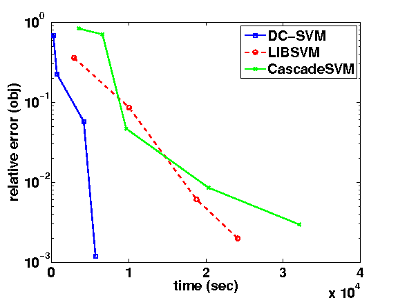
(a) webspam objective function

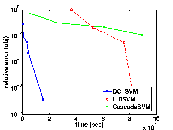
(b) covtype objective function

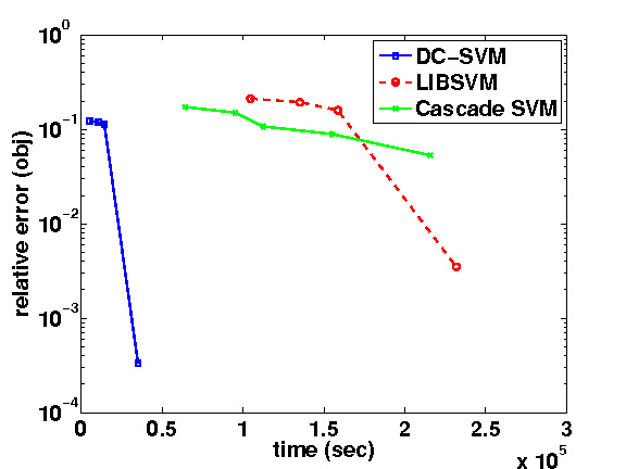
(c) mnist8m objective function

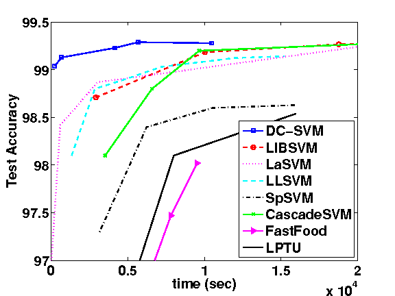
(d) webspam testing accuracy

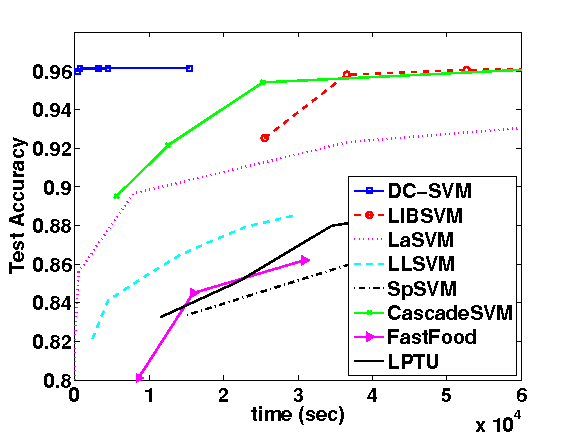
(e) covtype testing accuracy

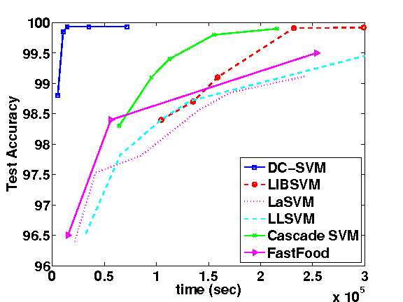
(f) mnist8m testing accuracy

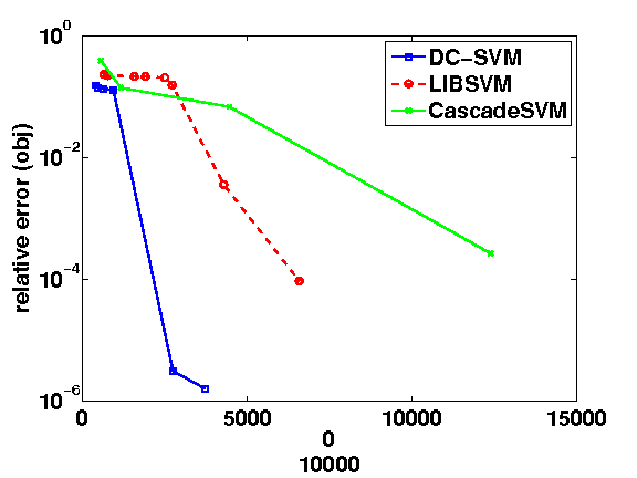
(g) kddcup99 objective function

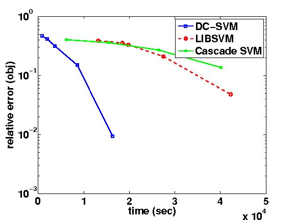
(h) cifar objective function

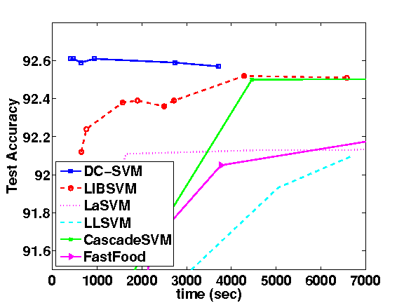
(i) kddcup99 testing accuracy

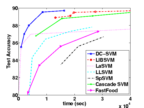
(j) cifar testing accuracy

Figure 3: Comparison of algorithms using the RBF kernel. Each point for DC-SVM indicates the result when stopping at different levels; each point for LIBSVM and CascadeSVM indicates different stopping conditions; each point for LaSVM indicates various number of passes through data points; each point for LTPU and LLSVM, and FastFood indicates different sample sizes; and each point for SpSVM indicates different number of basis vectors. Methods with testing performance below the bottom of the y-axis are not shown in the figures.

Experimental Results with RBF kernel: Table 3 presents time taken and test accuracies. Experimental results show that the early prediction approach in DC-SVM achieves near-optimal test performance. By going to the top level (handling the whole problem), DC-SVM achieves better test performance but needs more time. Table 3 only gives the comparison on one setting; it is natural to ask, for example, about the performance of LIBSVM with a looser stopping condition, or Fastfood with varied number of Fourier features. Therefore, for each algorithm we change the parameter settings and present more detailed results in Figure 3.

Figure 3 shows convergence results with time – in 3a, 3b, 3c the relative error on the y-axis is defined as $(f(\boldsymbol{\alpha})-f(\boldsymbol{\alpha}^{*}))/f(\boldsymbol{\alpha}^{*})$, where $\boldsymbol{\alpha}^{*}$ is computed by running LIBSVM with $10^{-8}$ accuracy. Online and approximate solvers are not included in this comparison as they do not solve the exact kernel SVM problem. We observe that DC-SVM achieves faster convergence in objective function compared with the state-of-the-art exact SVM solvers. Moreover, DC-SVM is also able to achieve superior test accuracy in lesser training time as compared with approximate solvers. Figure 3d, 3e, 3f compare the efficiency in achieving different testing accuracies. We can see that DC-SVM consistently achieves more than 50 fold speedup while achieving higher testing accuracy.

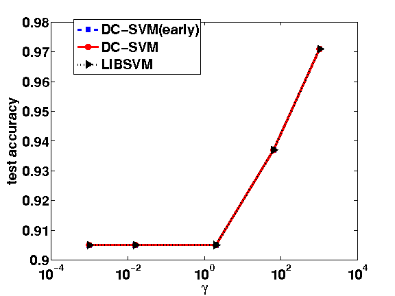
(a) ijcnn1 $C=2^{-10}$

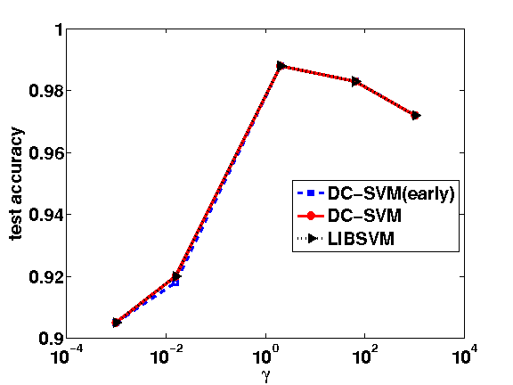
(b) ijcnn1 $C=2^{1}$

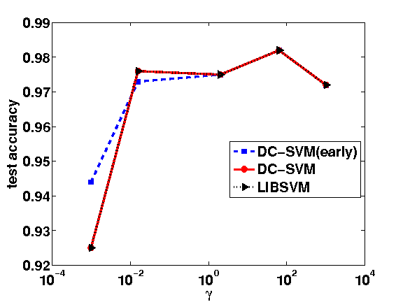
(c) ijcnn1 $C=2^{10}$

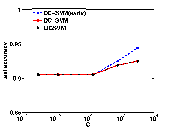
(d) ijcnn1 $\gamma=2^{-10}$

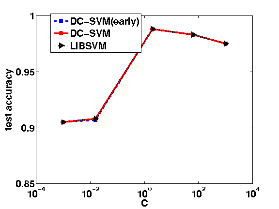
(e) ijcnn1 $\gamma=2^{1}$

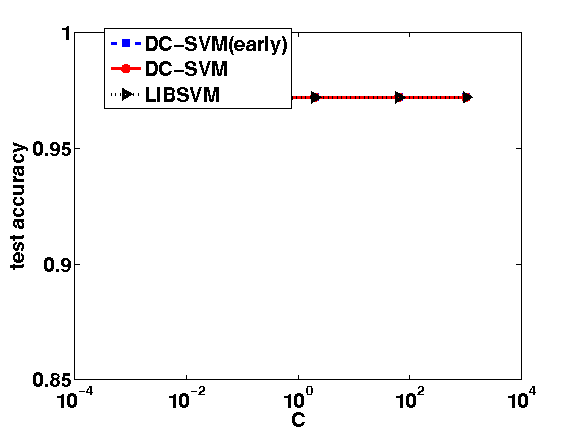
(f) ijcnn1 $\gamma=2^{10}$

Figure 5: Robustness to the parameters $C,\gamma$ on ijcnn1 dataset.

Experimental Results with varying values of $C,\gamma$: As shown in Theorem 1 the quality of approximation depends on $D(\pi)$, which is strongly related to the kernel parameters. In the RBF kernel, when $\gamma$ is large, a large portion of kernel entries will be close to 0, and $D(\pi)$ will be small so that $\bar{\alpha}$ is a good initial point for the top level. On the other hand, when $\gamma$ is small, $\bar{\alpha}$ may not be close to the optimal solution. To test the performance of DC-SVM under different parameters, we conduct the comparison on a wide range of parameters ($C=[2^{-10},2^{-6},2^{1},2^{6},2^{10}],\gamma=[2^{-10},2^{-6},2^{1},2^{6},2^{10}]$). The results on the ijcnn1, covtype, webspam and census datasets are shown in Tables 7, 8, 9, 10 (in the appendix). We observe that even when $\gamma$ is small, DC-SVM is still 1-2 times faster than LIBSVM: among all the 100 settings, DC-SVM is faster on 96/100 settings. The reason is that even when $\bar{\alpha}$ is not close to $\alpha$, using $\bar{\alpha}$ as the initial point is still better than initialization with a random or zero vector. On the other hand, DC-SVM (early) is extremely fast, and achieves almost the same or even better accuracy when $\gamma$ is small (as it uses an approximated kernel). In Figure 5, 7, 6, 8 (in appendix) we plot the performance of DC-SVM and LIBSVM under various $C$ and $\gamma$ values, the results indicate that DC-SVM (early) is more robust to parameters. The accumulated runtimes are shown in Table 5.

Experimental Results with the polynomial kernel: To show that DC-SVM is efficient for different types of kernels, we further conduct experiments on covtype and webspam datasets for the degree-3 polynomial kernel $K({\boldsymbol{x}}_{i},{\boldsymbol{x}}_{j})=(\eta+\gamma{\boldsymbol{x}}_{i}^{T}{\boldsymbol{x}}_{j})^{3}$. For the polynomial kernel, the parameters chosen by cross validation are $C=2,\gamma=1$ for covtype, and $C=8,\gamma=16$ for webspam. We set $\eta=0$, which is the default setting in LIBSVM. Figures 4a and 4c compare the training speed of DC-SVM and LIBSVM for reducing the objective function value while Figures 4b and 4d show the testing accuracy compared with LIBSVM and LaSVM. Since LLSVM, FastFood and LPTU are developed for shift-invariant kernels, we do not include them in our comparison. We can see that when using the polynomial kernel, our algorithm is more than 100 times faster than LIBSVM and LaSVM. One main reason for such large improvement is that it is hard for LIBSVM and LaSVM to identify the right set of support vectors when using the polynomial kernel. As shown in Figure 2, LIBSVM cannot even identify 20% of the support vectors in $10^{5}$ seconds, while DC-SVM has a very good guess of the support vectors even at the bottom level, where number of clusters is 256.

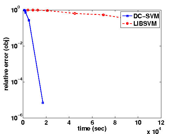
(a) webspam objective function

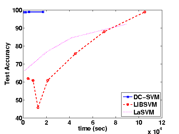
(b) webspam testing accuracy

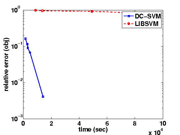
(c) covtype objective function

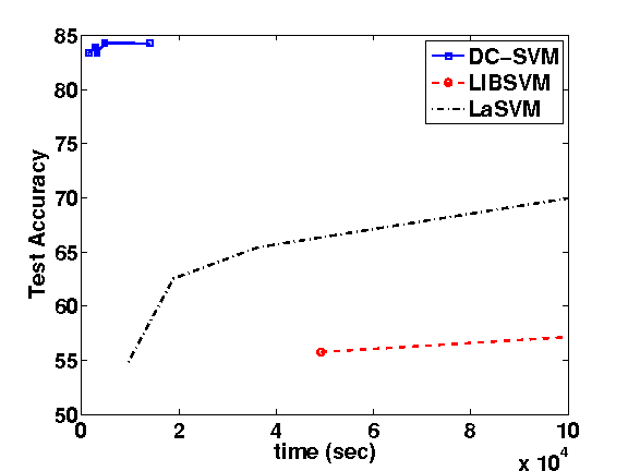
(d) covtype testing accuracy

Figure 4: Comparison of algorithms on real datasets using the polynomial kernel.

Clustering time vs Training time. Our DC-SVM algorithm is composed of two important parts: clustering and SVM training. In Table 6 we list the time taken by each part; we can see that the clustering time is almost constant at each level, while the rest of the training time keeps increasing.

Table 5: Total time for DC-SVM, DC-SVM (early) and LIBSVM on the grid of parameters $C,\gamma$ shown in Tables 7, 8, 9, and 10 (in the Appendix).

dataset	DC-SVM	DC-SVM	LIBSVM
	(early)
ijcnn1	16.4 mins	2.3 hours	6.4 hours
webspam	5.6 hours	4.3 days	14.3 days
covtype	10.3 hours	4.8 days	36.7 days
census	1.5 hours	1.4 days	5.3 days

Table 6: Run time (in seconds) for DC-SVM on different levels (covtype dataset). We can see the clustering time is only a small portion compared with the total training time.

Level	4	3	2	1	0
Clustering	43.2s	42.5s	40.8s	38.1s	36.5s
Training	159.4s	439.7s	1422.8s	3135.5s	7614.0s

6 Conclusions

In this paper, we have proposed a novel divide and conquer algorithm for solving kernel SVMs (DC-SVM). Our algorithm divides the problem into smaller subproblems that can be solved independently and efficiently. We show that the subproblem solutions are close to that of the original problem, which motivates us to “glue” solutions from subproblems in order to efficiently solve the original kernel SVM problem. Using this, we also incorporate an early prediction strategy into our algorithm. We report extensive experiments to demonstrate that DC-SVM significantly outperforms state-of-the-art exact and approximate solvers for nonlinear kernel SVM on large-scale datasets. The code for DC-SVM is available at http://www.cs.utexas.edu/~cjhsieh/dcsvm.

Table 7: Comparison of DC-SVM, DC-SVM (early), and LIBSVM on ijcnn1 with various parameters $C,\gamma$. DC-SVM (early) is always 10 times faster than LIBSVM and achieves similar test accuracy. DC-SVM is faster than LIBSVM for almost every setting.

dataset	$C$	$\gamma$	DC-SVM (early)		DC-SVM		LIBSVM		LaSVM
			acc(%)	time(s)	acc(%)	time(s)	acc(%)	time(s)	acc(%)	time(s)
ijcnn1	$2^{-10}$	$2^{-10}$	90.5	12.8	90.5	120.1	90.5	130.0	90.5	492
ijcnn1	$2^{-10}$	$2^{-6}$	90.5	12.8	90.5	203.1	90.5	492.5	90.5	526
ijcnn1	$2^{-10}$	$2^{1}$	90.5	50.4	90.5	524.2	90.5	1121.3	90.5	610
ijcnn1	$2^{-10}$	$2^{6}$	93.7	44.0	93.7	400.2	93.7	1706.5	92.4	1139
ijcnn1	$2^{-10}$	$2^{10}$	97.1	39.1	97.1	451.3	97.1	1214.7	95.7	1711
ijcnn1	$2^{-6}$	$2^{-10}$	90.5	7.2	90.5	84.7	90.5	252.7	90.5	531
ijcnn1	$2^{-6}$	$2^{-6}$	90.5	7.6	90.5	161.2	90.5	401.0	90.5	519
ijcnn1	$2^{-6}$	$2^{1}$	90.7	10.8	90.8	183.6	90.8	553.2	90.5	577
ijcnn1	$2^{-6}$	$2^{6}$	93.9	49.2	93.9	416.1	93.9	1645.3	91.3	1213
ijcnn1	$2^{-6}$	$2^{10}$	97.1	40.6	97.1	477.3	97.1	1100.7	95.5	1744
ijcnn1	$2^{1}$	$2^{-10}$	90.5	14.0	90.5	305.6	90.5	424.9	90.5	511
ijcnn1	$2^{1}$	$2^{-6}$	91.8	12.6	92.0	254.6	92.0	367.1	90.8	489
ijcnn1	$2^{1}$	$2^{1}$	98.8	7.0	98.8	43.5	98.8	111.6	95.4	227
ijcnn1	$2^{1}$	$2^{6}$	98.3	34.6	98.3	584.5	98.3	1776.5	97.8	1085
ijcnn1	$2^{1}$	$2^{10}$	97.2	94.0	97.2	523.1	97.2	1955.0	96.1	1691
ijcnn1	$2^{6}$	$2^{-10}$	92.5	27.8	91.9	276.3	91.9	331.8	90.5	442
ijcnn1	$2^{6}$	$2^{-6}$	94.8	19.9	95.6	313.7	95.6	219.5	92.3	435
ijcnn1	$2^{6}$	$2^{1}$	98.3	6.4	98.3	75.3	98.3	59.8	97.5	222
ijcnn1	$2^{6}$	$2^{6}$	98.1	48.3	98.1	384.5	98.1	987.7	97.1	1144
ijcnn1	$2^{6}$	$2^{10}$	97.2	51.9	97.2	530.7	97.2	1340.9	95.4	1022
ijcnn1	$2^{10}$	$2^{-10}$	94.4	146.5	92.5	606.1	92.5	1586.6	91.7	401
ijcnn1	$2^{10}$	$2^{-6}$	97.3	124.3	97.6	553.6	97.6	1152.2	96.5	1075
ijcnn1	$2^{10}$	$2^{1}$	97.5	10.6	97.5	50.8	97.5	139.3	97.1	605
ijcnn1	$2^{10}$	$2^{6}$	98.2	42.5	98.2	338.3	98.2	1629.3	97.1	890
ijcnn1	$2^{10}$	$2^{10}$	97.2	66.4	97.2	309.6	97.2	2398.3	95.4	909

Table 8: Comparison of DC-SVM, DC-SVM (early) and LIBSVM on webspam with various parameters $C,\gamma$. DC-SVM (early) is always more than 30 times faster than LIBSVM and has comparable or better test accuracy; DC-SVM is faster than LIBSVM under all settings.

dataset	$C$	$\gamma$	DC-SVM (early)		DC-SVM		LIBSVM
			acc(%)	time(s)	acc(%)	time(s)	acc(%)	time(s)
webspam	$2^{-10}$	$2^{-10}$	86	806	61	26324	61	45984
webspam	$2^{-10}$	$2^{-6}$	83	935	61	22569	61	53569
webspam	$2^{-10}$	$2^{1}$	87.1	886	91.1	10835	91.1	34226
webspam	$2^{-10}$	$2^{6}$	93.7	1060	92.6	6496	92.6	34558
webspam	$2^{-10}$	$2^{10}$	98.3	1898	98.5	7410	98.5	55574
webspam	$2^{-6}$	$2^{-10}$	83	793	68	24542	68	44153
webspam	$2^{-6}$	$2^{-6}$	84	762	69	33498	69	63891
webspam	$2^{-6}$	$2^{1}$	93.3	599	93.5	15098	93.1	34226
webspam	$2^{-6}$	$2^{6}$	96.4	704	96.4	7048	96.4	48571
webspam	$2^{-6}$	$2^{10}$	98.3	1277	98.6	6140	98.6	45122
webspam	$2^{1}$	$2^{-10}$	87	688	78	18741	78	48512
webspam	$2^{1}$	$2^{-6}$	93	645	81	10481	81	30106
webspam	$2^{1}$	$2^{1}$	98.4	420	99.0	9157	99.0	35151
webspam	$2^{1}$	$2^{6}$	98.9	466	98.9	5104	98.9	28415
webspam	$2^{1}$	$2^{10}$	98.3	853	98.7	4490	98.7	28891
webspam	$2^{6}$	$2^{-10}$	93	759	80	24849	80	64121
webspam	$2^{6}$	$2^{-6}$	97	602	83	21898	83	55414
webspam	$2^{6}$	$2^{1}$	98.8	406	99.1	8051	99.1	40510
webspam	$2^{6}$	$2^{6}$	99.0	465	98.9	6140	98.9	35510
webspam	$2^{6}$	$2^{10}$	98.3	917	98.7	4510	98.7	34121
webspam	$2^{10}$	$2^{-10}$	97	1350	82	31387	82	81592
webspam	$2^{10}$	$2^{-6}$	98	1127	86	34432	86	82581
webspam	$2^{10}$	$2^{1}$	98.8	463	98.8	10433	98.8	58512
webspam	$2^{10}$	$2^{6}$	99.0	455	99.0	15037	99.0	75121
webspam	$2^{10}$	$2^{10}$	98.3	831	98.7	7150	98.7	59126

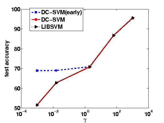
(a) covtype $C=2^{-10}$

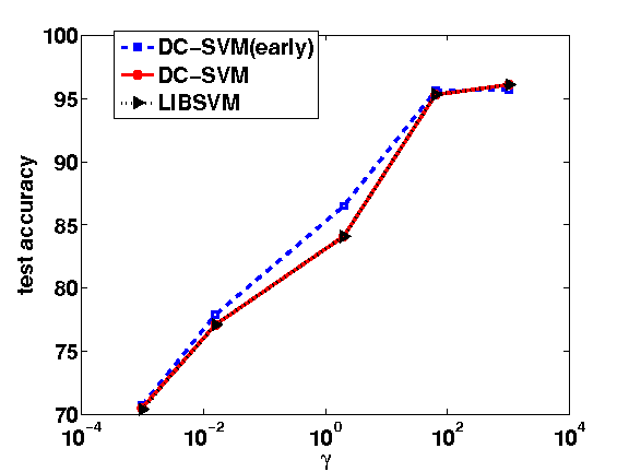
(b) covtype $C=2^{1}$

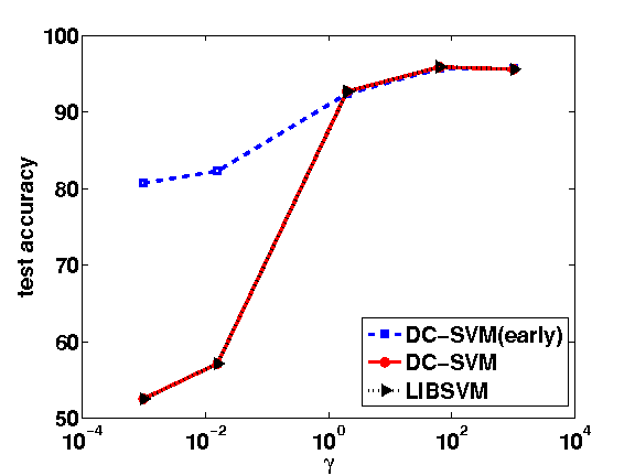
(c) covtype $C=2^{10}$

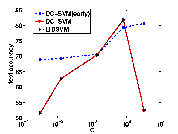
(d) covtype $\gamma=2^{-10}$

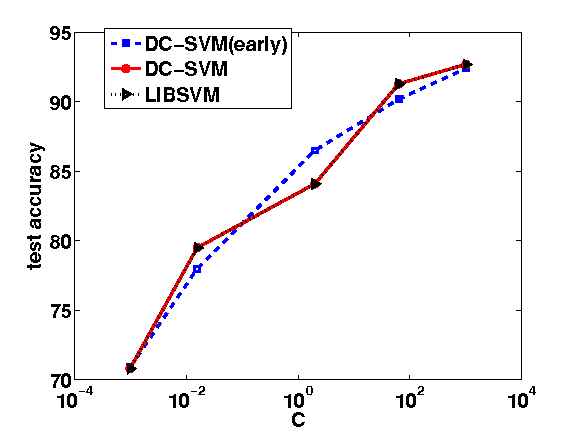
(e) covtype $\gamma=2^{1}$

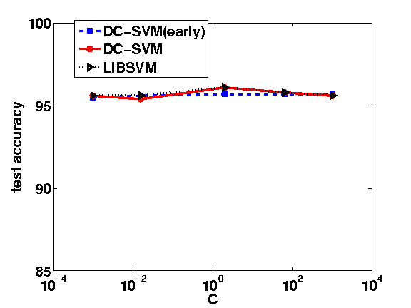
(f) covtype $\gamma=2^{10}$

Figure 6: Robustness to the parameters $C,\gamma$ on covtype dataset.

Table 9: Comparison of DC-SVM, DC-SVM (early) and LIBSVM on covtype with various parameters $C,\gamma$. DC-SVM (early) is always more than 50 times faster than LIBSVM with similar test accuracy; DC-SVM is faster than LIBSVM under all settings.

dataset	$C$	$\gamma$	DC-SVM (early)		DC-SVM		LIBSVM
			acc(%)	time(s)	acc(%)	time(s)	acc(%)	time(s)
covtype	$2^{-10}$	$2^{-10}$	68.9	736	51.5	24791	51.5	48858
covtype	$2^{-10}$	$2^{-6}$	69.0	507	62.7	17189	62.7	62668
covtype	$2^{-10}$	$2^{1}$	70.9	624	70.8	12997	70.8	88160
covtype	$2^{-10}$	$2^{6}$	86.7	1351	86.7	13985	86.7	85111
covtype	$2^{-10}$	$2^{10}$	95.5	1173	95.6	9480	95.6	54282
covtype	$2^{-6}$	$2^{-10}$	69.3	373	62.7	10387	62.7	90774
covtype	$2^{-6}$	$2^{-6}$	70.0	625	68.6	14398	68.6	76508
covtype	$2^{-6}$	$2^{1}$	78.0	346	79.5	5312	79.5	77591
covtype	$2^{-6}$	$2^{6}$	87.9	895	87.9	8886	87.9	120512
covtype	$2^{-6}$	$2^{10}$	95.6	1238	95.4	7581	95.6	123396
covtype	$2^{1}$	$2^{-10}$	70.7	433	70.4	25120	70.4	88725
covtype	$2^{1}$	$2^{-6}$	77.9	1000	77.1	18452	77.1	69101
covtype	$2^{1}$	$2^{1}$	86.5	421	84.1	11411	84.1	50890
covtype	$2^{1}$	$2^{6}$	95.6	299	95.3	8714	95.3	117123
covtype	$2^{1}$	$2^{10}$	95.7	882	96.1	5349		$>$300000
covtype	$2^{6}$	$2^{-10}$	79.3	1360	81.8	34181	81.8	105855
covtype	$2^{6}$	$2^{-6}$	81.3	2314	84.3	24191	84.3	108552
covtype	$2^{6}$	$2^{1}$	90.2	957	91.3	14099	91.3	75596
covtype	$2^{6}$	$2^{6}$	96.3	356	96.2	9510	96.2	92951
covtype	$2^{6}$	$2^{10}$	95.7	961	95.8	7483	95.8	288567
covtype	$2^{10}$	$2^{-10}$	80.7	5979	52.5	50149	52.5	235183
covtype	$2^{10}$	$2^{-6}$	82.3	8306	57.1	43488		$>$ 300000
covtype	$2^{10}$	$2^{1}$	92.4	4553	92.7	19481	92.7	254130
covtype	$2^{10}$	$2^{6}$	95.7	368	95.9	12615	95.9	93231
covtype	$2^{10}$	$2^{10}$	95.7	1094	95.6	10432	95.6	169918

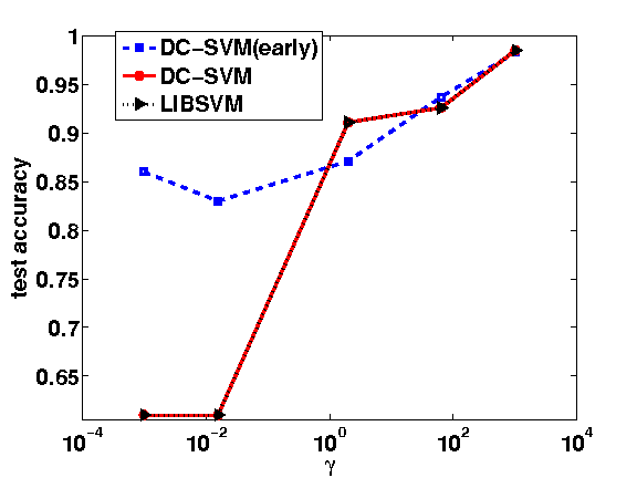
(a) webspam $C=2^{-10}$

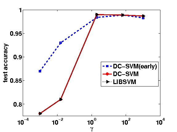
(b) webspam $C=2^{1}$

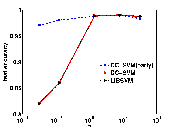
(c) webspam $C=2^{10}$

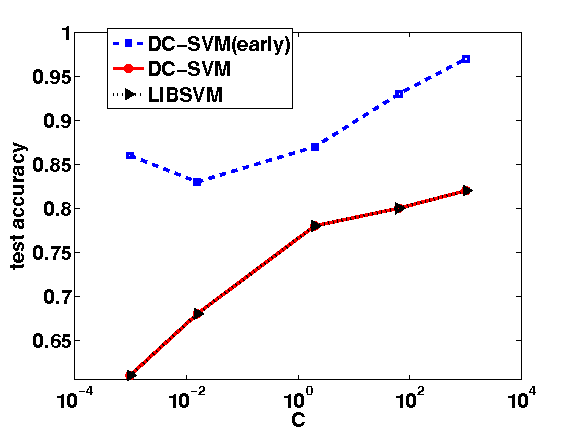
(d) webspam $\gamma=2^{-10}$

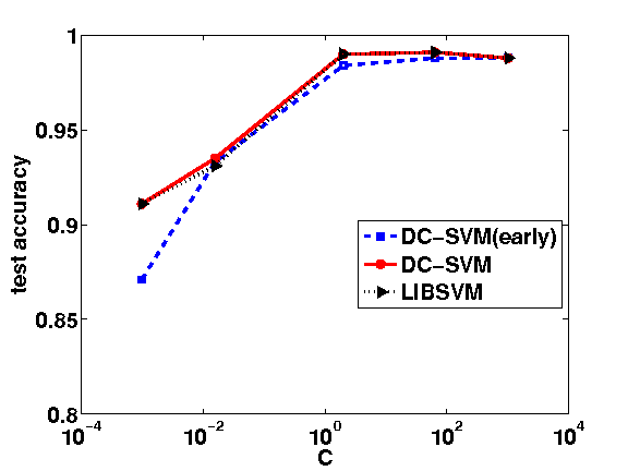
(e) webspam $\gamma=2^{1}$

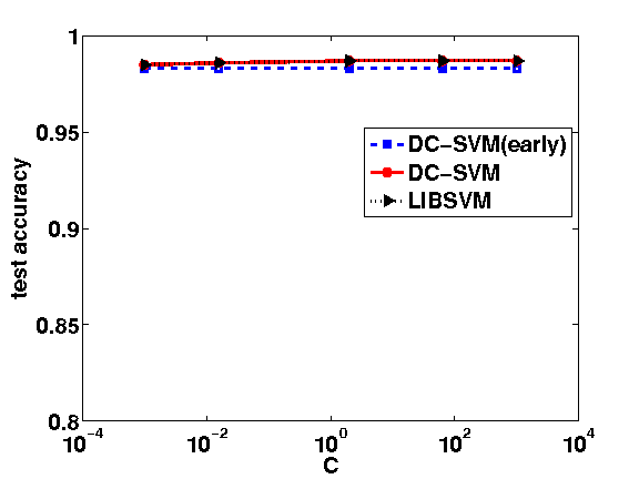
(f) webspam $\gamma=2^{10}$

Figure 7: Robustness to the parameters $C,\gamma$ on webspam dataset.

Table 10: Comparison of DC-SVM, DC-SVM (early) and LIBSVM on census with various parameters $C,\gamma$. DC-SVM (early) is always more than 50 times faster than LIBSVM with similar test accuracy; DC-SVM is faster than LIBSVM under all settings.

dataset	$C$	$\gamma$	DC-SVM (early)		DC-SVM		LIBSVM
			acc(%)	time(s)	acc(%)	time(s)	acc(%)	time(s)
census	$2^{-10}$	$2^{-10}$	93.80	161	93.80	2153	93.80	3061
census	$2^{-10}$	$2^{-6}$	93.80	166	93.80	3316	93.80	5357
census	$2^{-10}$	$2^{1}$	93.61	202	93.68	4215	93.66	11947
census	$2^{-10}$	$2^{6}$	91.96	228	92.08	5104	92.08	12693
census	$2^{-10}$	$2^{10}$	62.00	195	56.32	4951	56.31	13604
census	$2^{-6}$	$2^{-10}$	93.80	145	93.80	3912	93.80	6693
census	$2^{-6}$	$2^{-6}$	93.80	149	93.80	3951	93.80	6568
census	$2^{-6}$	$2^{1}$	93.63	217	93.66	4145	93.66	11945
census	$2^{-6}$	$2^{6}$	91.97	230	92.10	4080	92.10	9404
census	$2^{-6}$	$2^{10}$	62.58	189	56.32	3069	56.31	9078
census	$2^{1}$	$2^{-10}$	93.80	148	93.95	2057	93.95	1908
census	$2^{1}$	$2^{-6}$	94.55	139	94.82	2018	94.82	1998
census	$2^{1}$	$2^{1}$	93.27	179	93.36	4031	93.36	37023
census	$2^{1}$	$2^{6}$	91.96	220	92.06	6148	92.06	33058
census	$2^{1}$	$2^{10}$	62.78	184	56.31	6541	56.31	35031
census	$2^{6}$	$2^{-10}$	94.66	193	94.66	3712	94.69	3712
census	$2^{6}$	$2^{-6}$	94.76	164	95.21	2015	95.21	3725
census	$2^{6}$	$2^{1}$	93.10	229	93.15	6814	93.15	32993
census	$2^{6}$	$2^{6}$	91.77	243	91.88	9158	91.88	34035
census	$2^{6}$	$2^{10}$	62.18	210	56.25	9514	56.25	36910
census	$2^{10}$	$2^{-10}$	94.83	538	94.83	2751	94.85	8729
census	$2^{10}$	$2^{-6}$	93.89	315	92.94	3548	92.94	12735
census	$2^{10}$	$2^{1}$	92.89	342	92.92	9105	92.93	52441
census	$2^{10}$	$2^{6}$	91.64	244	91.81	7519	91.81	34350
census	$2^{10}$	$2^{10}$	61.14	206	56.25	5917	56.23	34906

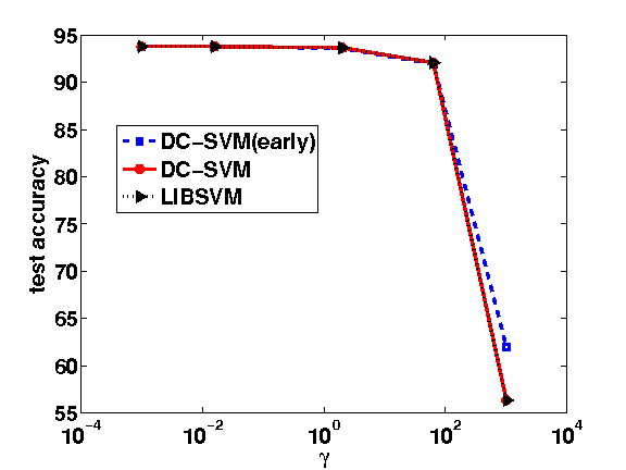
(a) census $C=2^{-10}$

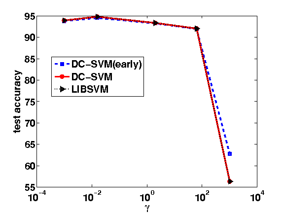
(b) census $C=2^{1}$

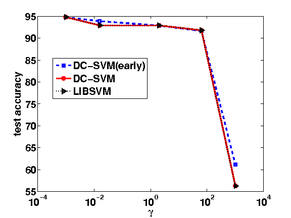
(c) census $C=2^{10}$

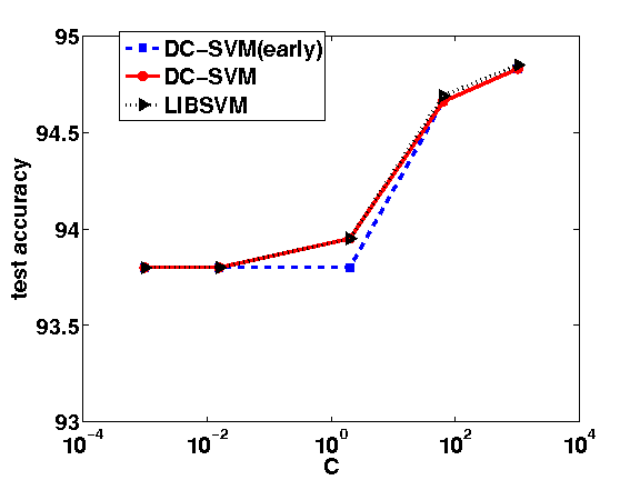
(d) census $\gamma=2^{-10}$

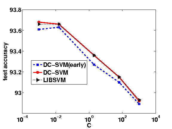
(e) census $\gamma=2^{1}$

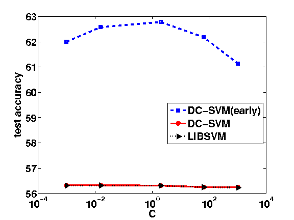
(f) census $\gamma=2^{10}$

Figure 8: Robustness to the parameters $C,\gamma$ on census dataset.

References

- Boley and Cao (2004) D. Boley and D. Cao. Training support vector machine using adaptive clustering. In SDM, 2004.
- Bordes et al. (2005) A. Bordes, S. Ertekin, J. Weston, and L. Bottou. Fast kernel classifiers with online and active learning. JMLR, 6:1579–1619, 2005.
- Chang and Lin (2011) Chih-Chung Chang and Chih-Jen Lin. LIBSVM: A library for support vector machines. ACM Transactions on Intelligent Systems and Technology, 2:27:1–27:27, 2011.
- Collobert et al. (2002) R. Collobert, S. Bengio, and Y. Bengio. A parallel mixture of SVMs for very large scale problems. In NIPS, 2002.
- Cortes and Vapnik (1995) C. Cortes and V. Vapnik. Support-vector networks. Machine Learning, 20:273–297, 1995.
- Fine and Scheinberg (2001) S. Fine and K. Scheinberg. Efficient SVM training using low-rank kernel representations. JMLR, 2:243–264, 2001.
- Ghitta et al. (2011) Radha Ghitta, Rong Jin, Timothy C. Havens, and Anil K. Jain. Approximate kernel k-means: Solution to large scale kernel clustering. In KDD, 2011.
- Graf et al. (2005) H. P. Graf, E. Cosatto, L. Bottou, I. Dundanovic, and V. Vapnik. Parallel support vector machines: The cascade SVM. In NIPS, 2005.
- Jacobs et al. (1991) R. A. Jacobs, M. I. Jordan, S. J. Nowlan, and G. E. Hinton. Adaptive mixtures of local experts. Neural Computation, 3(1):79–87, 1991.
- Joachims (1998) T. Joachims. Making large-scale SVM learning practical. In Advances in Kernel Methods – Support Vector Learning, pages 169–184, 1998.
- Joachims (2006) T. Joachims. Training linear SVMs in linear time. In KDD, 2006.
- Jose et al. (2013) C. Jose, P. Goyal, P. Aggrwal, and M. Varma. Local deep kernel learning for efficient non-linear SVM prediction. In ICML, 2013.
- Keerthi et al. (2006) S. S. Keerthi, O. Chapelle, and D. DeCoste. Building support vector machines with reduced classifier complexity. JMLR, 7:1493–1515, 2006.
- Kugler et al. (2006) M. Kugler, S. Kuroyanagi, A. S. Nugroho, and A. Iwata. CombNET-III: a support vector machine based large scale classifier with probabilistic framework. IEICE Trans. Inf. and Syst., 2006.
- Le et al. (2013) Q. V. Le, T. Sarlos, and A. J. Smola. Fastfood – approximating kernel expansions in loglinear time. In ICML, 2013.
- Loosli et al. (2007) Gaëlle Loosli, Stéphane Canu, and Léon Bottou. Training invariant support vector machines using selective sampling. In Large Scale Kernel Machines, pages 301–320. 2007.
- Moody and Darken (1989) John Moody and Christian J. Darken. Fast learning in networks of locally-tuned processing units. Neural Computation, pages 281–294, 1989.
- Pavlov et al. (2000) D. Pavlov, D. Chudova, and P. Smyth. Towards scalable support vector machines using squashing. In KDD, pages 295–299, 2000.
- Pérez-Cruz et al. (2004) F. Pérez-Cruz, A. R. Figueiras-Vidal, and A. Artés-Rodríguez. Double chunking for solving SVMs for very large datasets. In Proceedings of Learning 2004, Spain, 2004.
- Platt (1998) J. C. Platt. Fast training of support vector machines using sequential minimal optimization. In Advances in Kernel Methods - Support Vector Learning, 1998.
- Smola et al. (2007) A. Smola, S. Vishwanathan, and Q. Le. Bundle methods for machine learning. NIPS, 2007.
- Tresp (2000) V. Tresp. A Bayesian committee machine. Neural Computation, 12:2719–2741, 2000.
- Tsang et al. (2005) I.W. Tsang, J.T. Kwok, and P.M. Cheung. Core vector machines: Fast SVM training on very large data sets. JMLR, 6:363–392, 2005.
- Wang et al. (2011) Z. Wang, N. Djuric, K. Crammer, and S. Vucetic. Trading representability for scalability: Adaptive multi-hyperplane machine for nonlinear classification. In KDD, 2011.
- Yu et al. (2005) Hwanjo Yu, Jiong Yang, Jiawei Han, and Xiaolei Li. Making SVMs scalable to large data sets using hierarchical cluster indexing. Data Mining and Knowledge Discovery, 11(3):295–321, 2005.
- Zhang et al. (2008) K. Zhang, I. W. Tsang, and J. T. Kwok. Improved Nyström low rank approximation and error analysis. In ICML, 2008.
- Zhang et al. (2012) K. Zhang, L. Lan, Z. Wang, and F. Moerchen. Scaling up kernel SVM on limited resources: A low-rank linearization approach. In AISTATS, 2012.